Novel Recording Studio Features for Music Information Retrieval
←
→
Page content transcription
If your browser does not render page correctly, please read the page content below
Novel Recording Studio Features for Music Information Retrieval

                                                                                      Ziemer, Tim
                                                                  Bremen Spatial Cognition Center, University of Bremen
                                                                             ziemer@uni-bremen.de
                                                                             Kiattipadungkul, Pattararat
arXiv:2101.10201v1 [cs.SD] 25 Jan 2021

                                                     Faculty of Information and Communication Technology, Mahidol University
                                                                          pattararat.k@gmail.com
                                                                                 Karuchit, Tanyarin
                                                     Faculty of Information and Communication Technology, Mahidol University
                                                                  tanyarin.kar@student.mahidol.ac.th

                                                                                                Abstract
                                                   Producers of Electronic Dance Music (EDM) typically spend more time creating, shaping, mixing
                                               and mastering sounds, than with aspects of composition and arrangement. They analyze the sound by
                                               close listening and by leveraging audio metering and audio analysis tools, until they successfully created
                                               the desired sound aesthetics. DJs of EDM tend to play sets of songs that meet their sound ideal. We
                                               therefore suggest using audio metering and monitoring tools from the recording studio to analyze EDM,
                                               instead of relying on conventional low-level audio features. We test our novel set of features by a simple
                                               classification task. We attribute songs to DJs who would play the specific song. This new set of features
                                               and the focus on DJ sets is targeted at EDM as it takes the producer and DJ culture into account. With
                                               simple dimensionality reduction and machine learning these features enable us to attribute a song to a
                                               DJ with an accuracy of 63%. The features from the audio metering and monitoring tools in the recording
                                               studio could serve for many applications in Music Information Retrieval, such as genre, style and era
                                               classification and music recommendation for both DJs and consumers of electronic dance music.

                                               1.   INTRODUCTION
                                                      Electronic Dane Music (EDM) is a genre of music characterized as having a repetitive beat and
                                               synthesized backing audio [1]. EDM is an umbrella term, also referred to as electronica, techno or
                                               electro in their widest sense1 . EDM is produced primarily using electronic instruments and computers
                                               and is comprised of many subgenres and styles. EDM is often created and performed by Disc Jockeys
                                               (DJs) [2]. They generally select and mix EDM songs for broadcast, live performances in night clubs,
                                               concerts and on music festivals. Similarly to musical subgenres, the music that is curated by a DJ turns
                                               into a category of its own. The AllMusic Guide [3] describes “Electronic” music as “. . . a relentless
                                               desire to find a new sound no matter how tepid the results." [4, p. 107] puts it: “DJs such as Armin van
                                               Buuren, Paul van Dyk, Paul Oakenfold, Sasha and Tiësto pushed EDM into mainstream consciousness,
                                               [and] expanded the possibilities of the electronic dance soundscape (. . . ) the superstar DJ has become
                                               (. . . ) a significant arbiter of musical taste.” Consequently, many DJs stick to a certain sound rather than
                                               (sub-)genre. In practice, music producers achieve the desired sound by a combination of close listening
                                           1
                                             An overview can be found on http://techno.org/electronic-music-guide/. Note that we use the term without
                                         any implications concerning commercial intentions, level of originality, or artistic value.
and audio metering and monitoring tools in the recording studio. Furthermore, DJs contribute in steering,
shaping or even defining musical taste of many music listeners.
    In this paper we suggest a set of features derived from typical audio metering and analysis tools in
the music studio. These features should indicate a causal relationship between the objective acoustics
and the subjective sound preference of EMD producers and consumers. First, we analyze the music that
specific DJs integrated in their sets by means of the proposed features. Then, we train a machine learning
algorithm to estimate which music piece matches the sound ideal of which DJ, i.e., to predict which DJ
would play which song. In that sense, DJs are the classes, rather then genre or mood of a song. The
two facts that 1.) a DJ’s job is to select appropriate music for a large audience, and 2.) every DJ has
his/her own sound ideal, are a promising starting point for music classification that can serve, e.g., for
automatic music recommendation for EDM [5]. If a computer could identify a DJ’s sound ideal, it could
analyze millions of songs and recommend those songs that seem to meet this sound ideal. Such a music
recommendation approach could for example serve to enlarge the repertoire of a DJ by recommending
him/her matching but yet unknown music. Or it could serve as a music recommendation tool for music
consumers in music stores and streaming services. They would simply specify their favorite DJ and the
trained machine learning algorithm would recommend music that seems to meet this DJ’s sound ideal. It
could even serve the other wary round; as a DJ recommendation tool: A user lists some seed songs and
the machine could recommend him/her a DJ whose sound ideal matches the seed songs best.
    The remainder of this paper is structured as follows. Section 2 gives a broad overview about audio
content-based music classification and recommendation. Then, the music dataset we used is described in
detail in Section 3. Section 4 describes our method. It is subdivided into one subsection that explains the
selection of DJs, segmentation of music pieces and feature extraction. The second subsection describes
the dimensionality reduction and machine learning approach. The classification results are presented and
discussed in Section 5, followed by a conclusion in Section 6 and an outlook in Section 7.

2.   RELATED WORK
    Nowadays, online music stores and streaming services provide access to millions of songs. Both mu-
sic providers and customers need tools that organize the music and help the customer exploring unknown
songs finding music of their personal taste. Therefore, two topics are of relevance in Music Information
Retrieval (MIR) research; music classification and recommendation, which are briefly introduced in this
section based on some exemplary cases.

A.    ACOUSTICALLY-BASED GENRE CLASSIFICATION
    Automatic genre classification by means of acoustic features dates back to the early years of Music
Information Retrieval. One early example is [6], who extract about 10 features and test a number of
classifiers to classify music into 190 different genres with an accuracy of 61%. A large number of papers
addressed this problem, mostly focusing on improved redundancy reduction, feature selection and kernel
optimization for the classifier. One example is [7] who defined an elaborated kernel function for a support
vector machine (SVM) and test multiple feature selection and dimension reduction methods to achieve
a genre classification accuracy of 89.9% .
    However, [8] convicted most of these approaches as being a horse, i.e., classifying not based on
causal relationships between acoustic feature and genre, but based on statistical coincidences inherent in
the given dataset. This means, that many of the commonly extracted low-level features are meaningless
for the task of genre classification, and the classifier is not universally valid, i.e., it is not likely to perform
similarly well when applied to another dataset. Most importantly, a large number of publications showed
that sophisticated and elaborate machine learning approaches paired with extensive model testing can
tune classification accuracy from 60% to about 90%, even when the features are not explanatory for the
classes. This fact can lead to the erroneous assumption that an accurate classifier is a reliable and/or
explanatory classifier.
    Another weakness of automated genre classification is the lack of a valid ground truth. Genre and
style descriptions are debatable and may depend on aspects, such as decade, music scene, geographic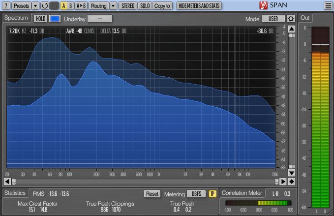
region, age, and many more [9]. In other words, genre, subgenres and styles are typologies, rather than
    classes. In contrast to classes, typologies are neither exhaustive nor mutually exclusive, not sufficiently
    parsimonious, based on arbitrary and ad hoc criteria and descriptive rather than explanatory or predictive
    [10]. A questionable ground truth is used to train a model. Consequently, the model output is at best
    questionable, too.
        In contrast to genre labels, DJ sets are a documented ground truth. However, it must be mentioned
    that DJs are not always free to play exclusively music that matches their sound ideal, but also music
    that is requested, e.g., by the audience or their record company. It is known that the nationality of DJs
    plays a certain role of influence on their performance style [11, p. 3 and 210]. Furthermore, DJs need to
    play new hit records and pre-released songs to stay exclusive and up-to-date. These circumstances may
    enforce them to play music that does not fully meet their aesthetic sound ideal. In addition to that, the
    taste and sound ideal of DJs is nothing static but may change over time.

    B.   ACOUSTICALLY-BASED MUSIC RECOMMENDATION
        Social services like Last.FM2 capture the music listening behavior of users and let them tag artists
    and songs from their local media library, which can serve as a basis for collaborative filtering based on
    tags and/or listening behavior. A common issues with collaborative filtering is the so-called cold start
    problem [12], i.e., new songs have only few listeners and no tags. This can be avoided by content-based
    music recommendation, e.g., based on metadata, such as artist, album, genre, country, music era, record
    label, etc. This approach is straight-forward, as these information are largely available in online music
    databases, like discogs3 . Services like musicube4 scrape information — e.g., about producer, songwriter,
    mood and instrumentation — to let end users of online music stores and streaming services discover a
    variety of music for all possible key terms and phrases. However, issue with recommendation based on
    music databases are the inconsistency of provided metadata and the subjectivity of some tags, especially
    mood- and genre-related tags. Acoustically-based music recommendation can avoid these issues, as they
    are based on acoustic features that can be extracted from any audio file.
         [12] let users rate the arousal, valence and resonance of music excerpts as a ground truth of music
    emotion. Then, they extract dozens of acoustic features and associate them with either of the dimensions.
    They use a dimensionality-reduction method to represent each dimension based on the associated fea-
    tures with minimum squared error. Finally, based on an analyzed seed song, the recommender suggests
    music pieces from a similar location within that three-dimensional space.
        Likewise, the MAGIX mufin music player analyzes a local music library and places every music
    piece at one specific location within a three-dimensional space based on audio features, see, e.g., [13,
    chap. 2]. Here, the three dimensions are labeled synthetic/acoustic, calm/aggressive, and happy/sad.
    The software recommends music from an online library that lies very near to a played seed song. The
    semantic space certainly makes sense, as it characterizes music in a rather intuitive and meaningful way.
    Drawbacks of the approach are that 1.) listeners may disagree with some of the rather subjective labels,
    2.) the transfer from extracted low-level features to semantic high-level features is not straight-forward
    and it can be observed that the leveraged algorithm often fails to allocate a music piece correctly, at least
    along the rather objective synthetic/acoustic-dimension.
         [14] extract over 60 common low-level features to characterize each song from a music library.
    Users create a seed playlist that they like. Then songs with a similar characteristic are recommended.
    The authors test different dimensionality reduction methods and distance models. In the most successful
    approach users rated 37.9% of the recommendations as good. Compared to that, recommending random
    songs with the same genre tag as most of the songs in the seed playlist created no less than 66.6% good
    recommendations. Still, the authors argue that their approach creates more interesting, unexpected and
    unfamiliar recommendations. This is desired because users need novel inspiration instead of obvious
    choices from a recommender.
2
  See https://www.last.fm.
3
  See https://www.discogs.com.
4
  See http://musicu.be.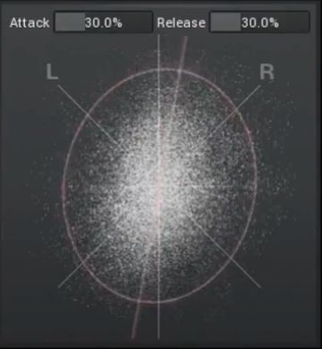
[15] aim to identify inter-subjective characteristics of music pieces leveraging psychoacoustic mod-
      els of loudness, roughness, sharpness, tonalness and spaciousness. A seed playlist is analyzed and then
      songs with similar psychoacoustic magnitudes are recommended. No machine learning is applied. In-
      stead, the psychoacoustic features are assumed as being orthogonal and a simple Euclidean distance is
      calculated. In a listening test, users rated 56% of the recommendations as good.
          It can be observed that all these music recommendation approaches focus on the music consumer.
      Due to our features and the focus on DJs of Electronic Dance Music, our classifier could serve as a basis
      for a music recommendation tool not only for music consumers but also for DJs.

      3.     THE DATASET
           For the sake of this study a small EDM database was created and analyzed.

      A.     DATA ACQUISITION
          When a disc jockey performs, he or she plays many songs in a single set. The scale of our dataset
      is as follows: in total, the 10 most popular DJs according to DJMag 5 were selected, each with 10 DJ
      sets. Each DJ set is about one to two hours long and consists of multiple tracks. The tracklist of each DJ
      set can be found on the 1001Tracklists website6 . As a result, a total of 1, 841 songs, often in a specific
      version or remix, were identified from 100 DJ sets. The artist names of the 10 DJs are:
        1.   Martin Garrix
        2.   Dimitri Vegas & Like Mike
        3.   Hardwell
        4.   Armin van Buuren
        5.   David Guetta
        6.   Dj Tiësto
        7.   Don Diablo
        8.   Afrojack
        9.   Oliver Heldens
       10.   Marshmello

      B.     DATA CLEANING
          We purchased all songs in the respective version or remix that we could find in online music stores;
      1, 262 songs in total. In a first step, the compressed audio files were decoded to PCM files with a sample
      rate of 44, 100 Hz, a sample depth of 16 bit and 2 channels. The file was cropped to remove silence in
      the beginning and at the end of the file, and then normalized to 0 dB, i.e.,

                                                   Max [|xm |] = 1 ,                                          (1)
      where xm represents the mth sample of the cropped PCM file, and can take values between −1 and
      1. Many club versions of songs begin and end with a rather stationary drum loop that makes it easier
      for a DJ to estimate the tempo, to blend multiple songs and to fade from one song to the next. We
      consider these parts as a practical offer to the DJ rather than a part of the creative sound design process.
      Consequently, we eliminate it by analyzing only the central 3 minutes of each song.
          The audio files were divided into segments of N = 212 = 4, 096 samples, which corresponds to
      about 93 ms. From each segment, a number of features was extracted. The features represent audio
      metering and monitoring tools that are commonly used in recording studios when mixing and mastering
      the music. They are introduced in the following section.
5
    See https://djmag.com/top100dj, retrieved June 4 2019.
6
    See https://www.1001tracklists.com, retrieved June 4 2019.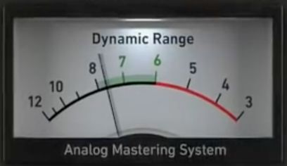
Figure 1: A screenshot of the VU meter                      Figure 2: A screenshot of the dy-
in the brainworx Shadow Hills Mastering                     namic range meter in the Brainworx
Compressor plugIn.                                          bx_masterdesk plugIn.

     4.    METHOD
         We analyze EDM through features that describe what audio metering and monitoring tools in the
     recording studio display. Producers of EDM use the same tools to create their desired sound. DJs make
     a selection of songs with matching sounds.

     A.    FEATURES
          Audio monitoring tools help music producers and audio engineers to shape the sound during music
     mixing and mastering [16–19]. For producers of EDM, the sound plays an exceptionally large role. They
     listen closely to the mix and consult such tools to achieve the desired sound in terms of temporal, spectral,
     and spatial aspects. Some audio monitoring tools are used on the complete stereo signal, whereas others
     are also applied to each third-octave band.

     i.    Volume Unit
         The Volume Unit (VU) meter [20, chap. 5], [17, chap. 7] is a volt meter, indicating an average
     volume level that had been standardized for broadcast between the 1940s and 1990s [18, chap. 12].
     Originally, an electric circuit deflected a mechanical needle. The inertia created a lag smearing that
     loosely approximated the signal volume over an integration time of 300 ms. In digital recording studios,
     a pseudo VU meter can be implemented by calculating
                                                          PD               !
                                                             d=1 |xd |
                                  VU = 20 log10 PD                             .                          (2)
                                                      d=1 |sin(2πt1000Hz)|

     Here, the denominator is a 1 kHz tone with maximum amplitude. Originally, D should be 13, 230
     samples at a sample rate of 44, 100 Hz, which corresponds to a duration of 300 ms. An example is
     illustrated in Fig. 1. In our case D = N .

     ii.   Peak Programme Meter
         The peak meter is the standard level meter [17, chap. 7]. The Peak Programme Meter (PPM) resem-
     bles a VU meter but has a much shorter integration time. In our digital case the PPM meter gives the
     peak value of a time frame
                                          PPM = 20 log10 (Max [|xn |]) .                              (3)
     In the recording studio these are displayed by bargraph meters [20, chap. 5], as can be seen in Fig. 3.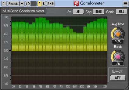
Figure 3: A screenshot of the
Steinberg Wavelab bargraph
meter indicating the current
level as a bar, the short-
term peak level as a single                                                     Figure 5: A screenshot of the
line above the bar, the over-                                                   FLUX:: Pure Analyzer plu-
all peak as a number in yel-                                                    gIn. Here, the pan of each fre-
low, and it indicated cipping                                                   quency band is indicated as a
by red LEDs.                                                                    horizontal deflection.

                                      Figure 4: A screenshot of
                                      the brainworx bx_meter plu-
                                      gIn, which indicates signal
                                      RMS, peak, DR, channel corre-
                                      lation and balance.

      iii.   Dynamic Range
         The Dynamic Range (DR) indicator [16, chap. 3] expresses the dynamic range within one time
      segment as ratio between lowest and largest peak within sub-segments si of 10 ms duration as

                                                            Max [si ]
                                          DR = 20 log10                 .                          (4)
                                                            Min [si ]

      One DR meter is illustrated in Fig. 2. It is related to the crest factor, also referred to as peak-to-average
      ratio [17, p. 293]. Both are low for mellow instruments and rise with increasing percussiveness [21].
          The above-mentioned audio metering tools are typically applied on single tracks and the complete
      master output. The audio monitoring tools in the following sections are applied to the complete audio as
      well as to each individual third-octave band.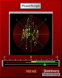
Figure 6: A screenshot of the Voxengo SPAN plugIn, which indicates the peak (dark blue) and RMS (light
blue) of each third octave band, together with the full bandwidth peak, RMS, crest factor and channel
correlation.

     iv.   Third-Octave Bands
         In addition to the complete audio, the following audio monitoring tools are also applied on each of
     the 27 third-octave bands around the center frequencies 40, 50, 63, 80, 100, 125, 160, 200, 250, 315,
     400, 500, 630, 800, 1000, 1250, 1600, 2000, 2500, 3150, 4000, 5000, 6300, 8000, 10000, 12500, and
     16000 Hz [20, chap. 13] filtered according to the ANSI s1.11 standard [22].

     v.    Root Mean Square
        In the recording studio the Root Mean Square (RMS) of the audio time series is used to approximate
     loudness [18, chap. 5], [17, pp. 301ff]. The RMS is the quadratic mean calculated as
                                                     s
                                                         PD      2
                                                            d=1 xd
                                               RMS =               ,                                   (5)
                                                             D

     where xd represents the dth sample in the PCM file. Audio monitoring tools, tend to indicate the RMS
     in combination with other audio meters, like DR, peak, channel correlation and channel balance, as
     illustrated in Fig. 4.

     vi.   Phase Scope Distribution
         The phase scopes, also referred to as vector scope or goniometer, simply plot the left over the right
     channel, tilted by 45◦ [18, chap. 18] [23], [17, chap. 7]. Music producers derive a lot of information
     from qualitative and quantitative phase scope analysis.
         In the recording studio, a distribution along a vertical line indicates positive channel correlation
     and thus mono compatibility. Vertical lines are perceived as narrow, clearly localizable sound sources.
     In contrast, a distribution along a horizontal line indicates negative channel correlation, which creates
     destructive interference in the stereo loudspeaker setup. The optimal mixture of clear and diffuse sound
     is an important aspect of the producers sound ideal and is achieved through close listening and qualitative
     analysis of the phase scope distribution.
         We imitate this qualitative analysis by using box counting as suggested in [24]. First, we divide the
     two-dimensional space into 20 times 20 boxes. Then, we count how many of the 400 boxes are occupied
     by one or more values. Figure 7 illustrates a phase scope plugin.
Figure 7: A screenshot of Figure 8: A screenshot Figure 9: A screenshot of the Voxengo
the Steinberg PhaseScope of the MeldaProduction Correlometer plugIn, which indicates the
plugin, which plots the MStereoProcessor plu- channel correlation for a variable time
left over the right channel gIn. This phase scope segment length in each third octave band.
for each time window (yel- meter indicates the stereo
low distribution on top) width of a complete mix
and indicates the current, with an ellipse and the
highest and lowest chan- pan is given by its major
nel correlation (horizon- diameter.
tal bar at the bottom).
vii. Phase Scope Panning
A second feature that is derived from the phase scope is the panning, i.e., the dominant angle in the
distribution. We calculate it by plotting the absolute value of the left against the absolute value of the right
channel and transforming the coordinates from Cartesian to polar coordinates. Then, we calculate the
mean angle. Typically, dominant kickdrums tend to attract the distribution near 0◦ , whereas reverberant
pads, strings and atmo sounds tend to create a somewhat random distribution. Figures 8 and 5 show two
audio monitoring tools that indicate the pan of single frequency bands and the complete signal.
viii. Channel Correlation
Another measure often implemented in phase scope tools is Pearson’s correlation coefficient P of the
two stereo channels [19, 24]. It is sometimes referred to as phase meter or correlation meter [17, chap.
7]. It can be calculated as
cov (L, R)
P = , (6)
σ (L) σ (R)
where L and R represent the left and right channel vectors, cov the covariance and σ the standard
deviation, or as
P = Max [|L ∗ R|] (7)
where the asterisk denoted the cross-correlation operation. Here high positive values indicate mono
compatibility, and a comparably narrow sound impression. Negative values indicate phase issues and
violation of mono compatibility.
Many producers like to keep the overall channel correlation near 0.1, whereas producers that like
prominent drum sounds may prefer much higher values, and producers of atmospheric sounds may even
aim at negative channel correlation. A channel correlation meter for third-octave bands is illustrated in
Fig. 9.B. DIMENSIONALITY REDUCTION
Together, the above-mentioned audio metering and monitoring tools yield a 146-dimensional feature
vector:
• 8 features à 2 channels: • 3 features on stereo: • 5 features à 27 bands:
VU Box counting RMS (left)
PPM Panning RMS (right)
DR Channel correlation Box counting
RMS Panning
Channel correlation
Each feature contains 1, 983 values: one value for each window. These features are not orthogonal,
but somewhat redundant.
A Principal Component Analysis (PCA) is applied to represent the the 146-dimensional space by the
one diagonal line that that minimizes the squared distance between the line and all data points, i.e., the
first principal component.
A PCA is an established, linear method for dimensionality reduction based on feature projection.
More sophisticated, non-linear dimensionality reduction approaches, such as self-organizing maps [25],
are out of scope of this paper, but may improve the information content, and thus the success of the
classification, a lot.
C. CLASSIFICATION
To test the usefulness of audio metering and monitoring tools as features for tasks related to EDM,
we use the tools to classify 10 different DJs. We use random forest model [26], which is made up of
hundreds or thousands of decision trees. Only a subset of all the features are considered for splitting each
node in each decision tree. The final predictions are made by averaging the predictions of each individual
tree. Model fitting was done using sklearn7 . For the classifier we applied 5-fold cross-validation, i.e., the
original sample is randomly partitioned into 5 equal sized subsamples.
D. TEST AND EVALUATION
Cross validation is used to evaluate the classification models. The dataset is then split from the dataset
with the train_test_split() function from the Python scikit-learn machine learning library to
separate the data into a training dataset and a testing dataset. 90% of the dataset was used for training
while the remaining 10% of the data was used for testing. The performance of classification predictive
model is evaluated using an accuracy score.
5. RESULTS AND DISCUSSION
The random forest algorithm returns an overal accuracy of 62.99%. The result shows that the highest
accuracy is achieved when n_estimators is 25, bootstrap is True and the criterion for classification
is set to entropy. Other parameters include the maximum depth of the tree of 15, the random state of
49, and the number of features to consider when looking for the best split is auto. Note that for auto,
√
max [features] = nfeatures .
Table 1 shows the confusion matrix of the DJs. In 8 out of 10 cases the most frequent model output
is the correct DJ. The two exceptions are Armin van Buuren and Hardwell. Armin van Buuren has
frequently been falsely labeled as Dj Tiësto in 5 out of 11 cases and Oliver Heldens as Don Diablo in 3
out of 11 cases. These confusions are not necessarily a weakness of the features or the machine learning.
Both artist pairs appear to be quite similar. Last.FM lists Dj Tiësto as the most similar Dj to Armin van
7
See https://scikit-learn.org/stable/.D. Vegas & L. Mike
Armin van Buuren
Oliver Heldens
Martin Garrix
David Guetta
Marshmello
Don Diablo
Hardwell
Dj Tiësto
precision
Afrojack
f1-score
recall
Predicted/Actual DJ
Martin Garrix 10 0 0 1 2 3 0 0 0 0 0.833 0.625 0.714
D. Vegas & L. Mike 0 6 0 1 0 0 0 1 1 1 0.667 0.600 0.632
Hardwell 0 1 0 1 0 1 0 0 0 0 0 0 0
Armin van Buuren 0 2 1 2 0 5 0 0 0 1 0.333 0.182 0.235
David Guetta 1 0 0 0 5 0 2 2 0 0 0.556 0.500 0.526
Dj Tiësto 1 0 1 0 0 12 2 0 0 0 0.480 0.750 585
Don Diablo 0 0 1 1 0 2 19 0 1 1 0.704 760 731
Afrojack 0 0 1 0 0 1 1 2 0 0 0.333 0.400 364
Oliver Heldens 0 0 0 0 1 0 3 1 6 0 0.667 0.545 0.600
Marshmello 0 0 0 1 1 0 0 0 1 17 0.850 0.850 0.850
support/avg. 16 10 3 11 11 16 25 5 11 20 0.634 0.622 0.619
Table 1: Confusion matrix of the random forest model.
Buuren and Don Diablo as most similar to Oliver Heldens8 . All three Hardwell examples have been
attributed to other DJs, which could be a result of the low number of Hardwell pieces in the test data.
The Table also shows the classification report of the random forest model. Precision is the ratio
ycorrect /freqy . It indicates how many musical pieces have been attributed to the specific DJ correctly,
divided by the total number of pieces that have been attributed to that DJ. This equals the number of
correct classifications (diagonal cells) divided by the sum of the respective column. Recall is the ratio
ycorrect /freqx . It describes how many musical pieces have been attributed to the specific DJ correctly,
divided by the total number of pieces from that specific DJ. This equals the number of correct classi-
fications (diagonal cells) divided by the sum of the respective row. Except for Dj Tiësto the precision
and recall scores of each DJ have a similar magnitude. Dj Tiësto has a good recall, but, as explained
above, the precision is somewhat lower because many songs from the Armin van Buuren sets have been
falsely attributed to him. Support means how many songs of the respective DJ’s sets occurred in the
evaluation dataset. It is evident that Hardwell and Afrojack are poorly classified due to the low number
of occurrences in the test dataset. The avg. indicates the average precision, support and f1-score values.
6. CONCLUSION
We proposed features derived from audio metering and monitoring tools commonly used in music
recording studios. In contrast to many conventional low-level features or psychoacoustically-motivated
features, these features are consulted by music producers and recording engineers in practice. We hy-
pothesize that such features can be valuable for music analysis, classification and recommendation, par-
ticularly in the field of electronic dance music, where sound plays a crucial role on a par with (or even
more important than) other aspects such as composition, arrangement and mood. We evaluate these
features by a classification task. An audio content-based classifier attributes songs to DJs who would
8
See https://www.last.fm/music/Tiesto/+similar and https://www.last.fm/music/Oliver+
Heldens/+similar – retrieved January 15 2021. On Last.FM artist similarity is based on user-generated tags [27].play the song. The success rate of 63% and the fact that classification errors can be explained by artist
similarity and the unbalanced data set are evidence that the proposed features give causal explanations
of a DJs’ sound ideal, which can be valuable for various music information retrieval tasks, such as sound
analysis, genre classification and music recommendation, and maybe even producer recognition.
7. OUTLOOK
The proposed set of features seems suitable to give some explanation of a DJ’s sound ideal from
the viewpoint of recording studio technology and practice. Combining the audio metering and monitor-
ing features with psychoacoustic features, which attempt to mimic the producer’s auditory perception
during close listening, might be the perfect match to achieve a deep understanding of music production
aesthetics, sound preference and musical taste. Naturally, it would be beneficial to validate the features
by means of a listening experiment, either with the respective DJs, or with listeners of electronic dance
music.
According to many music recording, mixing, and mastering engineers, sound plays an important role
for all types of music, not only for EDM [28, p. 400], [29, p. 240], [30, p. V]. It may be interesting
to see how the proposed features perform on other popular music, like pop, rock, hip-hop, jazz, and on
recordings of classical music, raaga, gamelan or sea shanty pieces.
ACKNOWLEDGMENTS
This work was supported by the Summer Research Internship Program, financed by Erasmus+ and
the Mahidol-Bremen Medical Informatics Research Unit (MIRU).
REFERENCES
[1] H. C. Rietveld, “Introduction,” in DJ Culture in the Mix, B. A. Attias, A. Gavanas, and H. C. Ri-
etveld, Eds. New York, NY and London: Bloomsburry, 2013, ch. 1, pp. 1–14.
[2] A. Gavanas and B. A. Attias, “Guest editor’s introduction,” Journal of Electronic Dance Music
Culture, vol. 3, no. 1 (Special Issue on the DJ), pp. 1–3, 2011.
[3] AllMusic. (2020) Electronic. https://www.allmusic.com/genre/electronic-ma0000002572
[4] M. M. Hall and N. Zukic, “The dj as electronic deterritorializer,” in DJ Culture in the Mix. Power,
Technology, and Social Change in Electronic Dance Music, B. A. Attias, A. Gavanas, and H. C.
Rietveld, Eds. New York, NY: Bloomsbury, 2013, pp. 103–122.
[5] T. Ziemer, P. Kiattipadungkul, and T. Karuchit, “Music recommendation based on acoustic features
from the recording studio,” The Journal of the Acoustical Society of America, vol. 148, no. 4, pp.
2701–2701, 2020. https://doi.org/10.1121/1.5147484
[6] G. Tzanetakis and P. Cook, “Musical genre classification of audio signals,” IEEE Speech Audio
Process., vol. 10, no. 5, pp. 293–302, July 2002.
[7] S.-C. Lim, J.-S. Lee, S.-J. Jang, S.-P. Lee, and M. Y. Kim, “Music-genre classification system based
on spectro-temporal features and feature selection,” IEEE Transactions on Consumer Electronics,
vol. 58, no. 4, pp. 1262–1268, Nov. 2012.
[8] B. L. Sturm, “A simple method to determine if a music information retrieval system is a ’horse’,”
IEEE. Trans. Multimedia, vol. 16, no. 6, pp. 1636–1644, 2014.
[9] C. McKay, “Musical genre classification: Is it worth pursuing and how can it be improved?” in
Proceedings of the 7th International Conference on Music Information Retrieval, 2006.
[10] K. D. Bailey, Typologies and Taxonomies. An Introduction to Classification Techniques. Thousand
Oaks, CA: SAGE, 1994.
[11] B. Owsinski, The Mixing Engineer’s Handbook, 2nd ed. Thomson Course Technology, 2006.[12] J. J. Deng and C. Leung, “Emotion-based music recommendation using audio features and user
playlist,” in 6th International Conference on New Trends in Information Science, Service Science
and Data Mining (ISSDM2012), Oct 2012, pp. 796–801.
[13] T. Ziemer, Psychoacoustic Music Sound Field Synthesis, ser. Current Research in Systematic
Musicology. Cham: Springer, 2020, no. 7. http://doi.org/10.1007/978-3-030-23033-3
[14] D. Bogdanov, M. Haro, F. Fuhrmann, E. Gomez, and P. Herrera, “Content-based music recommen-
dation based on user preference example,” in WOMRAD, 2010.
[15] T. Ziemer, Y. Yu, and S. Tang, “Using psychoacoustic models for sound analysis in music,” in
Proceedings of the 8th Annual Meeting of the Forum on Information Retrieval Evaluation, ser. FIRE
’16. New York, NY, USA: ACM, 2016, pp. 1–7. https://doi.org/10.1145/3015157.3015158
[16] M. Senior, Mixing Secrets For the Small Studio. Burlington, MA: Focal Press, 2011.
[17] M. Collins, Pro Tools 8: Music Production, Recording, Editing, and Mastering. Burlington, MA:
Focal Press, 2009.
[18] E. B. Brixen, Audio Metering. Measurements, Standards, and Practice, 3rd ed. Audio Engineering
Society Press, 2020.
[19] T. Ziemer, “Source width in music production. methods in stereo, ambisonics, and wave field
synthesis,” in Studies in Musical Acoustics and Psychoacoustics, ser. Current Research in Systematic
Musicology, A. Schneider, Ed. Cham: Springer, 2016, vol. 4, ch. 10, pp. 399–440. https://doi.org/
10.1007/978-3-319-47292-8_10
[20] F. Rumsey and T. McCormick, Sound and Recording, 6th ed. Focal Press, 2009.
[21] A. Schneider, “Perception of timbre and sound color,” in Springer Handbook of Systematic Mu-
sicology, R. Bader, Ed. Berlin, Heidelberg: Springer, 2018, pp. 687–725. http://doi.org/10.1007/
978-3-662-55004-5_32
[22] Specification for Octave-Band and Fractional-Octave-Band Analog and Digital Filters, Acoustical
Society of America Std. ANSI.s1.11., 2009. https://law.resource.org/pub/us/cfr/ibr/002/ansi.s1.11.
2004.pdf
[23] R. Mores, “Music studio technology,” in Springer Handbook of Systematic Musicology, R. Bader,
Ed. Berlin, Heidelberg: Springer, 2018, pp. 221–258. http://doi.org/10.1007/978-3-662-55004-5_
12
[24] C. Stirnat and T. Ziemer, “Spaciousness in music: The tonmeister’s intention and the listener’s
perception,” in KLG 2017. klingt gut! 2017 – international Symposium on Sound, ser. EPiC
Series in Technology, P. Kessling and T. G\"orne, Eds., vol. 1. EasyChair, 2019, pp. 42–51.
https://doi.org/10.29007/nv93
[25] M. Blaß and R. Bader, “Content-based music retrieval and visualization system for
ethnomusicological music archives,” in Computational Phonogram Archiving, R. Bader, Ed. Cham:
Springer International Publishing, 2019, pp. 145–173.http://doi.org/10.1007/978-3-030-02695-0_7
[26] L. Breiman, “Random forests,” Machine Learning, vol. 45, no. 1, pp. 5–32, 2001.
[27] P. Knees and M. Schedl, “A survey of music similarity and recommendation from music context
data,” ACM Transactions on Multimedia Computing, Communications and Applications, vol. 10,
no. 1, p. article number: 2, 2013.
[28] R. Snowman, Dance Music Manual, 2nd ed. Focal Press, 2009.
[29] C. Roads, Composing Electronic Music. A New Aesthetic. Oxford University Press, 2015.
[30] D. Gibson, The Art of Mixing. Thomson Course Technology, 2005.You can also read