Assessing the Sensitivity of Global Maize Price to Regional Productions Using Statistical and Machine Learning Methods
←
→
Page content transcription
If your browser does not render page correctly, please read the page content below
HYPOTHESIS AND THEORY
                                                                                                                                                published: 02 June 2021
                                                                                                                                        doi: 10.3389/fsufs.2021.655206

                                            Assessing the Sensitivity of Global
                                            Maize Price to Regional Productions
                                            Using Statistical and Machine
                                            Learning Methods
                                            Rotem Zelingher 1*, David Makowski 2 and Thierry Brunelle 3
                                            1
                                              Université Paris-Saclay, INRAE, AgroParisTech, Economie Publique, Thiverval-Grignon, France, 2 Université Paris-Saclay,
                                            INRAE, AgroParisTech, Applied Mathematics and Computer Science (UMR 518), Paris, France, 3 CIRAD, UMR CIRED,
                                            Nogent-sur-Marne, France

                                            Agricultural price shocks strongly affect farmers’ income and food security. It is therefore
                                            important to understand and anticipate their origins and occurrence, particularly for the
                                            world’s main agricultural commodities. In this study, we assess the impacts of yearly
                                            variations in regional maize productions and yields on global maize prices using several
                                            statistical and machine-learning (ML) methods. Our results show that, of all regions
                                            considered, Northern America is by far the most influential. More specifically, our models
                         Edited by:         reveal that a yearly yield gain of +8% in Northern America negatively impacts the global
                  Ademola Braimoh,          maize price by about –7%, while a decrease of –0.1% is expected to increase global
     World Bank Group, United States
                                            maize price by more than +7%. Our classification models show that a small decrease in
                         Reviewed by:
                           Hideyuki Doi,    the maize yield in Northern America can inflate the probability of maize price increase on
            University of Hyogo, Japan      the global scale. The maize productions in the other regions have a much lower influence
                   Jordan Chamberlin,
    The International Maize and Wheat
                                            on the global price. Among the tested methods, random forest and gradient boosting
      Improvement Center (CIMMYT),          perform better than linear models. Our results highlight the interest of ML in analyzing
                                 Kenya      global prices of major commodities and reveal the strong sensitivity of maize prices to
                   *Correspondence:         small variations of maize production in Northern America.
                      Rotem Zelingher
               rotem.zelingher@inrae.fr     Keywords: food-security, maize, agricultural commodity prices, regional productions, machine learning

                     Specialty section:
           This article was submitted to    1. INTRODUCTION
 Land, Livelihoods and Food Security,
                 a section of the journal   Over the past decade, the four components of food security - availability, stability, utilization, and
Frontiers in Sustainable Food Systems
                                            access - have become major sources of concern. At the turn of 2010, prices of main food crops in
          Received: 18 January 2021         the international markets have shown high variability, sometimes doubling in a short time frame
            Accepted: 27 April 2021         (Headey and Fan, 2010). For example, the price of maize increased by 75% from September 2007
           Published: 02 June 2021
                                            to May 2008 (Headey, 2011). Poor harvests and rising prices of agricultural commodities had
                              Citation:     contributed to triggering the hunger riots of 2007–2008 and the Arab Spring of 2011 (Headey and
         Zelingher R, Makowski D and        Martin, 2016). High levels of volatility in the food prices are now recognized to affect food security
      Brunelle T (2021) Assessing the
                                            for a growing number of households (Rosenzweig et al., 2001; Schmidhuber and Tubiello, 2007).
    Sensitivity of Global Maize Price to
Regional Productions Using Statistical
                                               Several reasons have been put forward to explain the food crises at the turn of the decade: low
     and Machine Learning Methods.          levels of food stocks, rising prices of inputs - particularly fertilizers - and growing demand for
 Front. Sustain. Food Syst. 5:655206.       biofuel (Headey and Fan, 2008). One of the reasons most frequently cited relates to idiosyncratic
     doi: 10.3389/fsufs.2021.655206         shocks on agricultural production at the regional level. It has been shown that extreme local

Frontiers in Sustainable Food Systems | www.frontiersin.org                        1                                              June 2021 | Volume 5 | Article 655206
Zelingher et al. Assessing Sensitivity of Global Maize Price
environmental conditions in 2007 and 2010 (e.g., droughts in Although it is difficult to predict precisely the extent to which
Russia and, extensive wildfires in Australia) and the resultant global scale price variations could affect local prices, it has been
declines in regional production greatly contributed to the spike in previously shown that shifts in international prices can transmit
global food prices (Tadasse et al., 2016). The heatwave in Russia into regional domestic prices (Headey and Fan, 2010). In a more
in the summer of 2007 and 2010 led to a significant drop in recent research, Kalkuhl (2016) suggests that there is a strong
local wheat production, which resulted in export restrictions and relationship between international prices and domestic ones,
subsequent tensions on international markets (Wegren, 2011). even when the global market trades with futures.
Restrictions on rice exports in India and Vietnam in 2007/2008 The objective of our study is (i) to identify the maize-
also led to substantial price increases on international markets producing regions having the largest influence on the global price
(Headey, 2011). of maize through their production and (ii) to quantify the effects
It is generally considered that increased interconnectivity in of regional production changes on global price changes. Under
global food markets can be a source of resilience, as seen in the the assumption that maize prices are largely driven by regional
recent Covid-19 outbreak, but also of vulnerability, particularly production shifts (Hertel et al., 2016), we train several statistical
when the agricultural production of a major exporter is affected. and machine learning models using publicly available regional
Least developed countries are particularly vulnerable as they may yearly production data and monthly price data. Monthly price
suffer greater import losses through their strong dependence on data are pertinent because maize prices do not tend to change on
imports for staple foods (Puma et al., 2015). In this case, we a daily or weekly basis but rather monthly (Dorosh et al., 2004;
speak of teleconnected supply shocks (d’Amour et al., 2016). Ochieng et al., 2019). Our input variables, i.e., regional maize
d’Amour et al. (2016) find that the Middle East is most sensitive to productions or yields, directly inform on the level of commodity
teleconnected supply shocks in wheat, Central America to supply supply, which is usually an unstable component of the market.
shocks in maize, and Western Africa to supply shocks in rice. The trained models are used to analyze the relationships between
In the future, climate change and the increasing frequency of regional maize production (or yield) and global prices, to identify
extreme weather events could make the food system even more the most and least influential producing regions in the maize
vulnerable to such teleconnected shocks. Several works study the global market, and finally to quantify the effect of regional
transmission of prices and price volatility from international to production (or yield) changes on global price changes.
domestic markets (Baquedano and Liefert, 2014; Kalkuhl, 2016). In our study, we chose to use a variety of statistical and
However, to our knowledge, no article has so far attempted to machine learning methods. The use of different methods has
quantify the inverse link, namely the sensitivity of the world price several advantages. First, it allows us to study the robustness of
to supply shocks at the regional level. the main conclusions to the data analysis method implemented.
The international maize market is a highly relevant case Second, it makes it possible to compare the precision of
study because maize is one of the most traded crops and different methods and to determine the most efficient ones.
plays an important role in food security in many countries. Our comparison of models thus contributes to improve our
Accurate identification of the most influential maize producing understanding of the determinants of maize price and to develop
regions would be potentially useful for decision-makers who operational and accessible predictive tools. In this way, our study
need to optimize both their dates of commodity purchases and is relevant for designing food security policies.
their stock usages (World-Bank, 2005). Although maize is the
most widely traded crop in the world, only a few countries
export their maize productions, suggesting that maize price 2. MATERIALS AND METHODS
might be impacted by the production of a small number of 2.1. Data
regions. As some countries rely heavily on maize imports to Historical annual yield (hectograms per hectare) and production
ensure food security (Wu and Guclu, 2013; Rouf Shah et al., (tons) data were obtained from the FAO data website (FAOSTAT)
2016), it is important to be able to anticipate price shocks for all years available (1961 to 2018) for 19 regional entities
for this commodity. Models have been developed to provide (defined by FAO) covering 242 countries. For further data
relatively short-term maize price projections relevant to many definitions and the sources of the variables included in our
stakeholders. For example, the WASDE forecasts are used for models, see Supplementary Table 2 in Appendix A.
risk calculation and design of the federal US crop insurance Data on maize global monthly price were extracted from
program (US-HR, 2009). These models were criticized because the World Bank’s commodity markets database as a US No.
of their complexity (Hoffman and Meyer, 2018) and, sometimes, 2 yellow free on board (FOB) Gulf of Mexico, U.S. nominal
because of their lack of accuracy (Warr, 1990; Hoffman, 2011; price, per metric ton units. Although this price is the traditional
Hoffman et al., 2015; Lusk, 2016). Other forecasting models are representative price for the maize produced in the US, this
run by private institutions, in particular by companies specialized quotation is also accepted as the leading benchmark price for the
in commodity trading. Auto-regressive methods are widely used international maize trade (FAO, 2021)1 .
to forecast food price in the academic literature (Shively, 1996;
Li et al., 2010). Although all these tools are certainly useful 1 The series of relative yearly maize price changes used in this paper is strongly
for forecasting maize prices, they provide little insights into correlated with the relative maize price changes obtained in other countries. For
the effects of regional maize production variations on global example, Argentina and Ukraine (correlation of about 0.75), according to the data
maize prices. made available in the GIEWS database of the FAO.
Frontiers in Sustainable Food Systems | www.frontiersin.org 2 June 2021 | Volume 5 | Article 655206Zelingher et al. Assessing Sensitivity of Global Maize Price
FIGURE 1 | Time series of global maize price. (A) Real terms in 2010 US Dollars. (B) Real terms in relative change from the same month of the previous year (ratio).
The time series summarizes the monthly price of maize, as and their values are shown in Figure 1B. From the series of pm,y ,
globally traded in FOB US Gulf ports, from January 1960 to we define a binary variable pbm,y equal to one in case of price
December 2019. We converted these prices into real 2010 US increase (pm,y > 0) and to zero otherwise.
Dollars, using the monthly agricultural index of the World-Bank2 Maize prices for month m in year y are estimated as a function
(Figure 1). of relative production (or yield) changes between the month m in
The real prices are further denoted as qm,y , where m and y year y and the same month in year y − 1. To accomplish this, we
are the month and year indices, respectively. Exportable maize transformed regional yield (grain weight per unit of the cropping
is usually harvested once a year, during the main harvest season, area, in hectograms per hectare) and production (total regional
and levels of maize production can thus potentially have strong grain weight, in tons) data into relative changes compared to the
effects on yearly price changes. For this reason, the dependent previous year, as follows:
variable in our analysis is defined as the relative price difference
of maize expressed relatively to the same month of the previous
year. It is defined as
zk,y − zk,y−1
xk,y = (2)
zk,y−1
qm,y − qm,y−1
pm,y = (1)
qm,y−1
Where zk,y is the production (or yield) in a region k (k=1, . . . , 19)
and year y, and xk,y is the relative production (or yield) change in
2 Although the most frequently use price index is the American CPI, we chose to the same region and the same year.
use the World-Bank monthly agricultural price index. We base our decision on two We predict prices during the last quarter of each year, that is in
factors: The first derives from Tadasse et al. (2016) indicating that the US CPI could October, November, and December (m ∈10,11,12), i.e., when all
be a biased deflator when dealing in a global market that includes both developed
and developing countries. The second reason is a relatively smaller gap (RMSE)
regions have finished (or almost finished) their maize harvest and
between the maize annual real prices as published by the World-Bank to the real reported the yearly production and yield obtained. For a given
maize global monthly price calculated for this study. year, it is indeed possible to obtain accurate estimates of maize
Frontiers in Sustainable Food Systems | www.frontiersin.org 3 June 2021 | Volume 5 | Article 655206Zelingher et al. Assessing Sensitivity of Global Maize Price
yield and production from October onward and to use them to repeatedly distributing the observations into homogeneous
predict price shocks of the same year3 . groups relative to pm,y . The partitioning criteria is monotonous
In the next sections, we present and compare several methods in the explanatory variable, xk , which defines a cross-section
to estimate pm,y and pbm,y at m ∈10,11,12 as a function of of xk , whereas higher valued observations belong to the right
xk,y , k ∈1,. . . ,19. Each method is implemented twice; first using branch and lower-valued to the left branch. Additional partitions
relative changes in regional productions as input variables and based on the same variable can be made, but at each stage,
then using relative yield changes. one cut-off point is determined. The subgroups that define the
tree are called nodes. CART performs recursive partitioning,
2.2. Linear and Generalized Linear Models and searches for splits that minimize the test error rate in
Although the relationships between price and production or yield the chosen objective function. The choice of the objective
changes may be non-linear, we use a linear regression model function depends on whether the output is continuous (pm,y ) or
as a benchmark to estimate price fluctuation as a function of categorical (pbm,y ). In the former case, i.e., for predicting pm,y ,
changes in regional productions or yields. Our linear model (LM) CART is implemented using the residual sum of squares (RSS).
is defined as follows: To predict pbm,y (classification), the objective function is a purity
index based on the Gini index. Here, CART was implemented
X
19
with the package rpart of the R software (Therneau et al., 2019)
pm,y = α + βk xk,y + ǫm,y (3)
(rpart function).
k=1
where α and βk are regression parameters and ǫm,y is the 2.4. Random Forest and Gradient Boosting
residuals. Additionally, we define a variant of this model Although simple to visualize and interpret, CART results are
including the price change of year y − 1 (i.e., pm,y−1 ) as usually unstable and tend to be sensitive to small data changes.
a supplementary input. This serves for investigating Granger Their price predictions are not always accurate (Kuhn and
causal relation between pm,y and xk,y (Granger, 1969). The Johnson, 2013). For these reasons, ensemble learning algorithms
significance of the effects of xk,y are tested with and without using based on bagging (for “bootstrap aggregating”) and boosting
pm,y−1 as an additional input in the regression model. If some of methods are frequently used instead of CART trees (Breiman,
the xk,y are still significant while taking pm,y−1 into account, one 2000). In this study we use Random-forest (RF) (Liaw and
can be considered that there is a Granger causal relation between Wiener, 2002) as a bagging-based algorithm, and gradient
pm,y and these xk,y . boosting machine (GBM) as a boosting-based method.
For classification, we use a generalized linear model (GLM) The RF algorithm builds an ensemble of trees, each relying on
with a binomial family and a logit link. This model computes the a small subset of inputs (i.e., a subset of all regional productions
probability that pbm,y =1 (i.e., price increase), given the values of or yields). Each tree is fitted to a randomly chosen training-set
the regional production (or yield) changes xk,y , k ∈1,. . . ,19. generated using a bootstrap procedure. This approach reduces
Both models are implemented with the glm function of R (R- the effects of correlations between variables while allowing
Core-Team, 2020). As done with the other methods, we fit linear different input variables to be selected. In RF, predictions are
models for each month (October, November, and December) derived by computing the average of all trees. Here, we find that
using successively production and yield changes as inputs. The 500 trees lead to stable results. RF can rank the inputs according
most influential inputs were selected using a stepwise procedure to their predictive powers and, here, the resulting ranking can
implemented with the AIC criterion (step function of R). be used to identify the regions whose maize productions (or
yields) show the strongest influence on maize global price. In this
2.3. CART study, RF is implemented with the randomForest function of
The three ML methods considered in this study are decision- the package randomForest (Breiman et al., 2018), both for
tree based algorithms: classification and regression trees (CART), quantitative predictions and for classification.
Random-forest (RF), and gradient boosting machine (GBM). The method GBM is also based on an ensemble of trees (Efron
None of these methods makes any strong assumption about and Hastie, 2016). At each iteration, GBM builds a simple tree
the functional form of the relationship between the dependent (weak-learner), each of which is learning from the prediction
variable and the explanatory variables, neither about the errors of all the trees built so far. The final prediction is expressed
data distribution. They are thus able to capture nonlinear as the sum of all the models calculated earlier. As RF, GBM
relationships between the inputs (regional production or yield is able to rank the inputs according to their predictive powers.
changes) and the output (global price change). We shortly In our case, we fit GBM using the gbm function of the gbm
present our implementation of CART here, while RF, and GBM package (Friedman, 2001) both for regression and classification
are presented in the next sections. based predictions. Here, we find that the most accurate results
The purpose of CART is to build a binary decision tree. are obtained with 100 trees for GBM.
Let pm,y be a dependent variable and x1,y , xk,y , . . . , xK,y a Neither RF or GBM have analytical expressions, but standard
series of explanatory variables. The tree is constructed by methods can be used to rank their inputs according to their
importance and visualize their effects on the output, here on
3 http://www.amis-outlook.org/amis-about/calendars/maizecal/en/, retrieved 23 price changes. Using these methods, we rank the model inputs
March 2020. xk,y from the most influential to the least by computing the mean
Frontiers in Sustainable Food Systems | www.frontiersin.org 4 June 2021 | Volume 5 | Article 655206Zelingher et al. Assessing Sensitivity of Global Maize Price
decrease accuracy criterion (Calle and Urrea, 2010) for each input Northern America is by far the most influential region according
(i.e., each regional production or yield changes). This criterion to the four methods, with both types of inputs (production
measures the extent to which the accuracy of model predictions or yield changes), and for the three months considered. The
or classifications decreases when each of the input variables is only exception is the linear model (with yield change inputs) in
set to a random value. Lastly, we use partial dependence plots November, but this model has low predictive power compared
(Greenwell, 2017) to visualize the response of the model outputs to others in November (Table 1). Considering the most accurate
to the most influential inputs, averaging the overall values of the methods (GBM and RF), yield and production changes in
other inputs. These plots allow us to analyze the shapes of the Northern America have the strongest influence on global price
responses and detect non-linearity. The same approaches were changes. Moreover, according to the linear models, the effects
applied to LM and CART to compare the input rankings and the of yield and production change in Northern America on global
dependence plots of all methods on the same basis. price change are statistically significant (p < 0.01) in October,
November, and December, with and without the price change in
2.5. Models Evaluation year y-1 included as an additional explanatory input. This result
The accuracy of the quantitative price-estimation is assessed by indicates a Granger causality of yield and production changes in
root mean squared error (RMSE), which we estimate using leave- Northern America on global maize price. It reveals that yield and
one-out cross-validation (LOOCV). In each step, one year of production changes are useful in forecasting price changes, even
price (pm,y , m=10,11,12) and production/yield (xk,y ) is extracted when previous price changes were taken into account.
from the original data set. Then, the four models (CART, RF, The partial dependence plot (PDP) shown in Figure 3
GBM, and GLM) are trained using the remaining 55 years, to presents the average response of price changes in October (10),
estimate the removed value of pm,y using the trained models. The November (11), and December (12) to variations of maize
procedure is performed 56 times—once for each year—to obtain yield compared to the previous year in the most influential
a set of 56 estimations for each tested model and each month region, i.e., Northern America (similar PDPs are shown in the
(m=10,11,12). Finally, a value RMSE is calculated for each model Supplementary Figure 16 using production instead of yield).
and each predicted month. The whole procedure is repeated The PDPs obtained using the four models consistently show that
twice, using regional maize production and regional maize yields an increase (decrease) of yield in Northern America leads to
as inputs, successively. a decrease (increase) of global price. In October, for example,
To evaluate the accuracy of the classification models, we an 8% rise of relative maize yield in Northern-America leads
apply the same LOOCV procedure, this time to calculate the to a reduction of maize price of 7% according to the gbm
area under the ROC curve (AUC). This criterion is commonly model, while a 0.1% decrease of relative maize yield in Northern
used to evaluate the performance of classification algorithms America is expected to increase the global price by 7% according
(Hernández-Orallo et al., 2012). An AUC higher than 0.5 to the same model. This result confirms the strong influence
indicates better performance than random classification. An of Northern American yield on global maize price. The PDPs
AUC equal to 1 reveals a perfect classification. obtained using the production and yield changes in other regions
show much weaker trends and much flatter curves (see, for
3. RESULTS example, the PDPs obtained for the region Southern Africa, in
Supplementary Figures 20, 21).
3.1. Quantitative Effects of Regional
Productions on Price Changes
Table 1 shows that the best methods are either RF or GBM,
depending on the considered month. For example, the most 3.2. Classification of Price Increase vs.
accurate predictions of global price changes in October (p10,y ) are Decrease
obtained by RF with an RMSE equal to 0.12. The least accurate Figure 4 shows the results that ROC analyses for the classification
results (i.e., the highest RMSE) are obtained either with the linear models for the three months considered. The results are in favor
model (LM) or with CART, depending on the month considered. of GBM and RF with AUC falling in the range of 0.7–0.8 for these
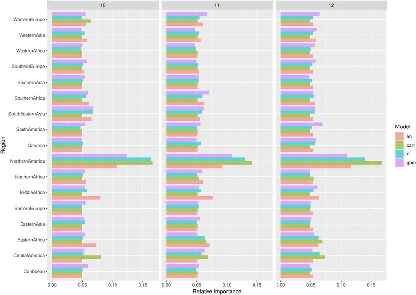
The importance ranking of the regional maize yields is shown methods in most cases. The 95%CI are relatively large but those
in Figure 2 for the three months considered and the four different obtained with RF and GBM never include the benchmark value
statistical and machine learning methods. The ranking obtained 0.5 characterizing a random classification. On the contrary, the
when using regional production changes as inputs is shown 95%CI of CART and the linear model sometimes include 0.5,
in the Supplementary Figure A.a.4. The relative importance of revealing that these methods do not systematically perform better
each region is determined by its contribution to the prediction than a random classification. For a given month and a given
accuracy (RMSE) of the price in a given month. A region is type of input, the lowest AUC is obtained by the linear model
considered influential if a random choice of its corresponding or CART. The two types of inputs did not lead to any systematic
input value (i.e., a yield change or production change chosen at difference in AUC values.
random) leads to a substantial increase of the RMSE of the price As already noticed in the case of regression, the importance
change predictions. On the other hand, a region is considered ranking of the regional production and yield inputs of the
non-influential if a random choice of its corresponding input classification models reveals that Northern America is the
value does not affect the RMSE. Results clearly show that most influential region, in particular for the model GBM
Frontiers in Sustainable Food Systems | www.frontiersin.org 5 June 2021 | Volume 5 | Article 655206Zelingher et al. Assessing Sensitivity of Global Maize Price
TABLE 1 | Comparison of RMSE values for the four types of models (lm: linear model; cart: regression tree; rf: random forest; gbm: gradient boosting model).
Production Yield
lm cart rf gbm lm cart rf gbm
October 0.169 0.140 0.137 0.135 0.132 0.136 0.122 0.128
November 0.153 0.148 0.140 0.135 0.163 0.147 0.139 0.158
December 0.144 0.148 0.130 0.129 0.139 0.129 0.129 0.147
RMSE values (expressed in the same unit as a relative price change, i.e., in relative change ratio compared to the same month the previous year), were computed by cross-validation
for predicting yearly price changes in October, November, and December using two types of inputs: relative regional production (left) or yield (right) changes. The lowest values obtained
for each month are in red.
FIGURE 2 | Importance levels of regional yield changes for predicting the global maize price in October (10), November (11), and December (12). Importance levels
are computed using the RMSE criterion and measure the extent to which the model accuracy decreases with a random permutation of each input.
which has a good classification power. For more details, see positive in Northern America compared to the previous year,
Figures A.a.5, A.a.5 in Supplementary Materials A.a.4. while it increases above 0.5 when the yield change is negative.
Figure 5 shows the PDPs of the classification models. These The effect is particularly strong with the model GBM. As already
PDPs represent the average responses of the probability of noticed for quantitative price changes, the PDPs obtained with
price increase to relative yield changes in Northern America the classification models show much weaker trends and much
(PDPs obtained with regional production inputs are shown in flatter curves for regions other than Northern America (see, for
Supplementary F). The probability of a global price increase example, the PDPs obtained for the region Southern Africa, in
strongly decreases below 0.5 as soon as the yield change is Supplementary Figures 22, 23).
Frontiers in Sustainable Food Systems | www.frontiersin.org 6 June 2021 | Volume 5 | Article 655206Zelingher et al. Assessing Sensitivity of Global Maize Price
FIGURE 3 | Partial dependence plots obtained with lm, cart, rf, and gbm showing the average response of relative price change in October (10), November (11), and
December (12) to relative yield change in Northern America. The points indicate price variations as observed over the period of 1961–2019. The plot shows that,
according to all models, any increase (decrease) of yield in Northern America compared to the previous year leads to a decrease (increase) of global price.
4. DISCUSSION us to quantify the effect of an increase or decrease in the
annual production of maize in this region on the global price
Using regional maize production data and global maize prices, of this commodity. All methods reveal that a small increase
we were able to assess the effects of regional production and (decrease) of maize production or yield in Northern America
yield variations on late-season global maize prices. Because of is expected to decrease (increase) the global maize price by a
the existing relationship between the global price and domestic few percent compared to the previous year. Considering the
prices, especially in the least developed countries (Caracciolo most accurate methods, an increase of maize yield relative to
et al., 2014), the topic is important to dealing with food security the previous year of +8% in Northern America negatively affect
issues in vulnerable regions. the global maize price by about –7%, while a decrease of yield
Our study is the first to address this question using a large in Northern America as low as –0.1% is expected to increase
variety of statistical and machine learning methods. Overall, global maize price by more than 7%. The strong impact of maize
all models consistently show that the most influential region is production in Northern America is confirmed by the results
Northern America, and both maize yields and maize productions obtained with the classification methods. Indeed, these methods
seem to be equally influential. This result is somewhat expected indicate that the small increase (decrease) in maize yield or
as Northern America (and, more specifically, the USA) is the production in Northern America has a strong negative (positive)
main maize producer and exporter at the global scale and effect on the probability of maize price increase compared
as the USA is known to have a strong influence on the to the previous year. Even a very small decrease in maize
agricultural trade market Chatzopoulos et al. (2019). However, production in Northern America can inflate the probability of a
our models provide data-driven quantitative information on price increase.
the effect of regional production variations on global maize Among all the considered modeling techniques, ensemble
prices. Our analysis provides real added value because it allows tree-based techniques (random forest and gradient boosting)
Frontiers in Sustainable Food Systems | www.frontiersin.org 7 June 2021 | Volume 5 | Article 655206Zelingher et al. Assessing Sensitivity of Global Maize Price FIGURE 4 | AUC values obtained for the classification models predicting price increase vs. price decrease in October (10), November (11), and December (12). The horizontal red line indicates AUC = 0.5, i.e random classification. Vertical bars indicate the 95% confidence intervals (CI). When these bars do not include 0.5, the AUC is significantly higher than 0.5 (p < 0.05). show the lowest root mean squared error and highest AUC production vs. yield changes). Thus, surprisingly, both GBM and values, revealing that these methods were the best for both RF do not perform better when regional production variations quantitative price prediction and classification. Indeed, in are used as inputs instead of yield. This is although production addition to being able to quantitatively predict price changes, data combine two types of information, i.e., yields and cropping the methods tested in this paper can be used to classify areas, whether yield variations alone do not account for possible relative price increase vs. decrease situations. The principle variance in the regional maize cultivated areas. is to compute the probability of price change increase (or Although the main purpose of our study is not to propose decrease) as a function of regional production (or yield) changes. new forecasting tools, our models could potentially be used The tree-based models tend to outperform the simpler GLM to predict global maize prices. Compared to other types of model. Still, the rate of misclassification is approximately 25% forecasting models, GBM and RF have several advantages but, with GBM and RF, which is relatively high but better than a also, a few disadvantages. Our models rely on public data and random classification. As noticed for quantitative predictions, can be easily implemented using standard modeling open-source the production change in Northern America is, by far, the software. On the contrary, private forecasting techniques are most influential input for classifying price increase vs. price usually unpublished, not freely available, and not transparent. decrease situations. All these results concur to show that maize Structural models constitute another category of models that can production change in Northern America is a highly relevant predict prices of agricultural commodities. These models rely indicator for assessing the risk of global maize price increase on theories describing economic systems and are developed by or decrease. international organizations such as FAO, OECD, and IFPRI. They The performances of the methods considered are only simulate price fluctuations using a series of functions describing marginally impacted by the nature of their inputs (i.e., partial or general market equilibrium. Although these models Frontiers in Sustainable Food Systems | www.frontiersin.org 8 June 2021 | Volume 5 | Article 655206
Zelingher et al.                                                                                                           Assessing Sensitivity of Global Maize Price

 FIGURE 5 | Partial dependence plots showing the probability of price increase in October, November, and December as a function of relative yield change in Northern
 America, for the four models considered. The points indicate price variations (on the y-axis, 1, price increase; 0, price decrease) as observed over the period of
 1961–2019.

are used to predict product prices in the long run, they are                         realistic to get reliable regional production data before the
not usually implemented to make short-term predictions. They                         end of summer. This with regards to regions located in the
are also complex and cannot be easily run by non-specialists.                        Northern hemisphere, in particular in Northern-America, which
The WASDE model is another example of an operational tool                            is a key region for predicting global maize price. For this reason,
for maize price predictions. Similarly to our models, WASDE                          all models were used here to predict global maize prices at
can forecast maize price at a monthly time step. According to                        the end of the year, more specifically in October, November,
Hoffman et al. (2015), WASDE relies on a combination of nine                         and December.
different structural and non-structural sub-models while GBM                             In this study, we analyzed the effect of regional productions
and RF can be easily implemented using free R packages and                           on global maize prices during the last three months of the
publicly accessible data. They could be thus easily run by any                       year. We made this choice to be consistent with the harvest
interested stakeholder and updated every year based on the most                      date for maize in the main maize-producing region—North
recent data.                                                                         America—which takes place in the very late summer and fall.
   In the future, our models could be adapted to predict price                       Although we did not carry out a detailed analysis for earlier
changes for other agricultural commodities from regional crop                        months, we did perform a sensitivity analysis of the influence
productions. From a practical point of view, a disadvantage of                       of North America depending on the month considered and
the ML tree-based models is that they rely on yearly regional                        found that this region retained a significant but lesser influence
production input data. In principle, these data are only available                   in the months preceding the harvest, probably due to the
after harvest, but relatively accurate values can be estimated                       influence of the harvest forecasts anticipated by the maize market
shortly before harvest from local expert knowledge and model                         players. In the future, however, it would be very useful to
predictions. Considering the maize growing season, it is not                         deepen this analysis to identify more precisely the influence of

Frontiers in Sustainable Food Systems | www.frontiersin.org                      9                                              June 2021 | Volume 5 | Article 655206
Zelingher et al.                                                                                                                     Assessing Sensitivity of Global Maize Price

the different producers on prices during the first months of                                of ML for predicting global prices of major commodities from
the year.                                                                                   regional production and assessing price sensitivity to regional
    Our approach could potentially be replicated for other crops                            crop producers.
whose production is less geographically concentrated. This would
allow us to assess the world food price sensitivity to production                           DATA AVAILABILITY STATEMENT
shocks or an export ban in a given country.
                                                                                            Publicly available datasets were analyzed in this study. This data
                                                                                            can be found here: http://www.fao.org/faostat/en/#data; https://
5. CONCLUSIONS                                                                              www.worldbank.org/en/research/commodity-markets.
This study demonstrates that it is possible to assess the impact
of regional maize production variations on the global price                                 AUTHOR CONTRIBUTIONS
of maize using machine-learning (ML) techniques on publicly
available regional production and price data. As these methods                              All authors listed have made a substantial, direct and intellectual
can be easily implemented using only freely available packages                              contribution to the work, and approved it for publication.
and public information, our results contribute to making the
forecasting of the global price of maize more accessible. As such,                          FUNDING
our price prediction technique can be included food security
management programs and policies and possibly serve as a price                              This study was funded by the French ANR project CLAND
forecaster. The methods considered can rank regional producers                              (16-CONV-0003) and by the INRAE metaprogram GloFoods.
according to their influence on global maize prices and our results
show that, out of all regions, Northern America is by far the                               SUPPLEMENTARY MATERIAL
most influential. More specifically, our results reveal that, for
maize, small positive production changes relative to the previous                           The Supplementary Material for this article can be found
year in Northern America have a strong and negative impact on                               online at: https://www.frontiersin.org/articles/10.3389/fsufs.
maize global price. Our study highlights the potential interest                             2021.655206/full#supplementary-material

REFERENCES                                                                                  Headey, D. (2011). Rethinking the global food crisis: the role of trade shocks. Food
                                                                                                Policy 36, 136–146. doi: 10.1016/j.foodpol.2010.10.003
Baquedano, F. G., and Liefert, W. M. (2014). Market integration and price                   Headey, D., and Fan, S. (2008). Anatomy of a crisis: the causes and
   transmission in consumer markets of developing countries. Food Policy 44,                    consequences of surging food prices. Agric. Econ. 39, 375–391.
   103–114. doi: 10.1016/j.foodpol.2013.11.001                                                  doi: 10.1111/j.1574-0862.2008.00345.x
Breiman, L. (2000). Randomizing outputs to increase prediction accuracy. Mach.              Headey, D., and Fan, S. (2010). Reflections on the global food crisis: how did it
   Learn. 40, 229–242. doi: 10.1023/A:1007682208299                                             happen? how has it hurt? and how can we prevent the next one? Intl. Food
Breiman, L., Cutler, A., Liaw, A., and Matthew, W. (2018). Breiman and Cutler’s                 Policy Res. Inst. 165, 142. doi: 10.2499/9780896291782RM165
   Random Forests for Classification and Regression. R package version 4.6-14.              Headey, D. D., and Martin, W. J. (2016). The impact of food prices
Calle, M. L., and Urrea, V. (2010). Letter to the editor: stability of random forest            on poverty and food security. Ann. Rev. Resou. Econ. 8, 329–351.
   importance measures. Brief. Bioinform. 12, 86–89. doi: 10.1093/bib/bbq011                    doi: 10.1146/annurev-resource-100815-095303
Caracciolo, F., Cembalo, L., Lombardi, A., and Thompson, G. (2014).                         Hernández-Orallo, J., Flach, P., and Ferri, C. (2012). A unified view of performance
   Distributional effects of maize price increases in malawi. J. Dev. Stud. 50,                 metrics: Translating threshold choice into expected classification loss. J. Mach.
   258–275. doi: 10.1080/00220388.2013.833319                                                   Learn. Res. 13, 2813–2869.
Chatzopoulos, T., Pérez Domínguez, I., Zampieri, M., and Toreti, A. (2019).                 Hertel, T. W., Baldos, U. L. C., and van der Mensbrugghe, D. (2016). Predicting
   Climate extremes and agricultural commodity markets: a global economic                       long-term food demand, cropland use, and prices. Ann. Rev. Resou. Econ. 8,
   analysis of regionally simulated events. Weather Clim. Extremes 27:100193.                   417–441. doi: 10.1146/annurev-resource-100815-095333
   doi: 10.1016/j.wace.2019.100193                                                          Hoffman, L., and Meyer, L. (2018). Forecasting the US season-average farm price of
d’Amour, C. B., Wenz, L., Kalkuhl, M., Steckel, J. C., and Creutzig, F.                         upland cotton: derivation of a futures price forecasting model. Electr. Outlook
   (2016). Teleconnected food supply shocks. Environ. Res. Lett. 11:035007.                     Rep. Econ. Res. Serv.
   doi: 10.1088/1748-9326/11/3/035007                                                       Hoffman, L. A. (2011). Using Futures Prices to Forecast US Corn Prices: Model
Dorosh, P. A., Subbarao, K., and Del Ninno, C. (2004). Food aid and food security               Performance With Increased Price Volatility, Chapter 7, New York, NY: Springer
   in the short and long run: country experience from asia and sub-saharan africa               New York, 107–132.
   (english). Working Paper 538, World Bank, Washington, DC.                                Hoffman, L. A., Etienne, X. L., Irwin, S. H., Colino, E. V., and Toasa, J. I. (2015).
Efron, B., and Hastie, T. (2016). Computer Age Statistical Inference Algorithms,                Forecast performance of wasde price projections for us corn. Agric. Econ. 46,
   Evidence, and Data Science. 1st edn, Cambridge University Press.                             157–171. doi: 10.1111/agec.12204
FAO (2021). Giews fpma tool monitoring and analysis of food prices.                         Kalkuhl, M. (2016). How Strong Do Global Commodity Prices Influence Domestic
Friedman, J. H. (2001). Greedy function approximation: a gradient boosting                      Food Prices in Developing Countries? A Global Price Transmission and
   machine. Annals Stat. 29, 1189–1232. doi: 10.1214/aos/1013203451                             Vulnerability Mapping Analysis. Cham: Springer International Publishing, 269–
Granger, C. W. J. (1969). Investigating causal relations by econometric models                  301.
   and cross-spectral methods. Econometrica 37, 424–438. doi: 10.2307/19                    Kuhn, M., and Johnson, K. (2013). Applied Predictive Modeling, Vol. 26. Springer.
   12791                                                                                    Li, G.-Q., Xu, S.-W., and Li, Z.-M. (2010). Short-term price forecasting for agro-
Greenwell, B. M. (2017). pdp: an r package for constructing partial dependence                  products using artificial neural networks. Agric. Agric. Sci. Procedia 1, 278–287.
   plots. R J. 9, 421–436. doi: 10.32614/RJ-2017-016                                            doi: 10.1016/j.aaspro.2010.09.035

Frontiers in Sustainable Food Systems | www.frontiersin.org                            10                                                June 2021 | Volume 5 | Article 655206
Zelingher et al. Assessing Sensitivity of Global Maize Price Liaw, A., and Wiener, M. (2002). Classification and regression by randomforest. R Therneau, T., Atkinson, B., Ripley, B., and Ripley, M. B. (2019). Package ‘rpart’. News 2, 18–22. R package version 4.1-15. Lusk, J. L. (2016). From farm income to food consumption: Valuing usda data US-HR (2009). Hearing to review the federal crop insurance program : hearing products. Technical report. before the subcommittee on general farm commodities and risk management Ochieng, D. O., Botha, R., and Baulch, B. (2019). Structure, conduct and of the committee on agriculture. performance of maize markets in malawi. Technical Report 29, Washington, Warr, P. G. (1990). Predictive performance of the world bank’s commodity price DC: IFPRI. projections. Agric. Econ. 4, 365–379. doi: 10.1016/0169-5150(90)90011-O Puma, M. J., Bose, S., Chon, S. Y., and Cook, B. I. (2015). Assessing the Wegren, S. K. (2011). Food security and russia’s 2010 drought. Eurasian Geogr. evolving fragility of the global food system. Environ. Res. Lett. 10:024007. Econ. 52, 140–156. doi: 10.2747/1539-7216.52.1.14 doi: 10.1088/1748-9326/10/2/024007 World-Bank (2005). Managing Food Price Risks and Instability in an Environment R-Core-Team (2020). R: A Language and Environment for Statistical Computing. of Market Liberalization (english). Technical report, Washington, DC: World Vienna, Austria: R Foundation for Statistical Computing. version 3.6.3. Bank. Rosenzweig, C., Iglesias, A., Yang, X., Epstein, P. R., and Chivian, E. Wu, F., and Guclu, H. (2013). Global maize trade and food security: (2001). Climate change and extreme weather events; implications for food implications from a social network model. Risk Analysis 33, 2168–2178. production, plant diseases, and pests. Glob. Change Hum. Health 2, 90–104. doi: 10.1111/risa.12064 doi: 10.1023/A:1015086831467 Rouf Shah, T., Prasad, K., and Kumar, P. (2016). Maize—a potential source Conflict of Interest: The authors declare that the research was conducted in the of human nutrition and health: a review. Cogent Food Agric. 2:1166995. absence of any commercial or financial relationships that could be construed as a doi: 10.1080/23311932.2016.1166995 potential conflict of interest. Schmidhuber, J., and Tubiello, F. N. (2007). Global food security under climate change. Proc. Natl. Acad. Sci. U.S.A. 104, 19703–19708. Copyright © 2021 Zelingher, Makowski and Brunelle. This is an open-access article doi: 10.1073/pnas.0701976104 distributed under the terms of the Creative Commons Attribution License (CC BY). Shively, G. E. (1996). Food price variability and economic reform: an arch approach The use, distribution or reproduction in other forums is permitted, provided the for ghana. Am. J. Agric. Econ. 78, 126–136. doi: 10.2307/1243784 original author(s) and the copyright owner(s) are credited and that the original Tadasse, G., Algieri, B., Kalkuhl, M., and Von Braun, J. (2016). “Drivers and triggers publication in this journal is cited, in accordance with accepted academic practice. of international food price spikes and volatility,” in Food Price Volatility and Its No use, distribution or reproduction is permitted which does not comply with these Implications for Food Security and Policy. Springer, Cham, 59–82. terms. Frontiers in Sustainable Food Systems | www.frontiersin.org 11 June 2021 | Volume 5 | Article 655206
You can also read