ALMI-A Generic Active Learning System for Computational Object Classification in Marine Observation Images - MDPI
←
→
Page content transcription
If your browser does not render page correctly, please read the page content below
sensors
Article
ALMI—A Generic Active Learning System for Computational
Object Classification in Marine Observation Images
Torben Möller * and Tim W. Nattkemper

                                           Biodata Mining Group, Bielefeld University, 33615 Bielefeld, Germany; tim.nattkemper@uni-bielefeld.de
                                           * Correspondence: tmoeller@cebitec.uni-bielefeld.de

                                           Abstract: In recent years, an increasing number of cabled Fixed Underwater Observatories (FUOs)
                                           have been deployed, many of them equipped with digital cameras recording high-resolution digital
                                           image time series for a given period. The manual extraction of quantitative information from these
                                           data regarding resident species is necessary to link the image time series information to data from
                                           other sensors but requires computational support to overcome the bottleneck problem in manual
                                           analysis. As a priori knowledge about the objects of interest in the images is almost never available,
                                           computational methods are required that are not dependent on the posterior availability of a large
                                           training data set of annotated images. In this paper, we propose a new strategy for collecting
                                           and using training data for machine learning-based observatory image interpretation much more
                                           efficiently. The method combines the training efficiency of a special active learning procedure
                                           with the advantages of deep learning feature representations. The method is tested on two highly
                                           disparate data sets. In our experiments, we can show that the proposed method ALMI achieves on
                                           one data set a classification accuracy A > 90% with less than N = 258 data samples and A > 80% after
                                           N = 150 iterations, i.e., training samples, on the other data set outperforming the reference method
                                           regarding accuracy and training data required.

                                    Keywords: active learning; classification; deep learning; marine image annotation
Citation: Möller, T.; Nattkemper, T.
ALMI—A Generic Active Learning
System for Computational Object
Classification in Marine Observation       1. Introduction
Images. Sensors 2021, 21, 1134.                  The human impact on the marine ecosystem has increased in recent decades [1]. Ac-
https://doi.org/10.3390/s21041134
                                           tivities that have a major impact include oil drilling, fishing, and wind turbine deployment.
                                           An important factor in monitoring marine biodiversity and maintaining sustainable fish
Academic Editor: Bogusław Cyganek
                                           stocks is marine imaging [2,3]. Possible applications are, for example, creating a time series
Received: 30 December 2020
                                           of different species by detecting and classifying species in the images. However, computa-
Accepted: 3 February 2021
                                           tional support is needed to make the best use of the vast amounts of data generated, e.g., by
Published: 6 February 2021
                                           stationary underwater observatories [4] or seafloor observation systems [5]. A lot of work
Publisher’s Note: MDPI stays neu-
                                           exists in the context of (semi-)automated detection and classification of species in marine
tral with regard to jurisdictional clai-
                                           images [3,6–12]. All these works employ some kind of machine learning algorithm to ren-
ms in published maps and institutio-       der a data-driven model of the task to be performed (like object detection or classification).
nal affiliations.                          Such a machine learning approach towards (semi-)automatic image interpretation requires
                                           a training set of images (or image patches) and expert annotations, usually represented
                                           as (taxonomic) labels associated with the images collected with some image annotation
                                           software such as BIIGLE 2.0 [13]. In almost all works published, these images are in fact
Copyright: © 2021 by the authors. Li-      image patches, marked by domain experts in large images showing an underwater scenery
censee MDPI, Basel, Switzerland.           containing multiple objects. The detection and extraction of these patches showing single
This article is an open access article
                                           objects can be done by experts, sometimes supported by computational methods that often
distributed under the terms and con-
                                           employ unsupervised learning [14–16] or even citizen scientists [17]. However, one task
ditions of the Creative Commons At-
                                           that cannot be supported straightforwardly with computational methods or non-experts is
tribution (CC BY) license (https://
                                           the final classification of objects to taxonomic categories or morphotypes, and this task is
creativecommons.org/licenses/by/
                                           addressed in this work.
4.0/).

Sensors 2021, 21, 1134. https://doi.org/10.3390/s21041134                                                    https://www.mdpi.com/journal/sensors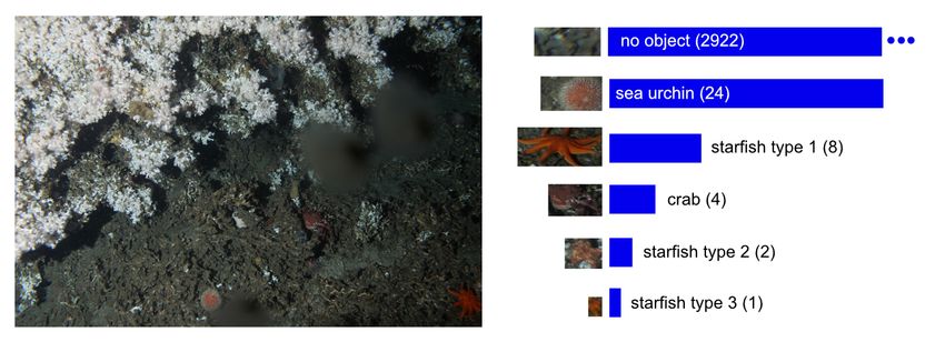
Sensors 2021, 21, 1134                                                                                               2 of 16

                              One main problem in providing computational support for taxonomic classification
                         by employing supervised learning classifiers is the amount of manual expert work required
                         to collect a training set of labeled image patches of sufficient size for all object classes.
                         To collect such a set, several challenges must be faced, some of them very special for
                         underwater computer vision applications:
                         1.   Limited background knowledge: Often, it is not known a priori which species can
                              occur in the data set.
                         2.   Expensive expert annotation: Quality controlled annotations are expensive in the
                              context of marine imaging because expert knowledge from the domain of marine
                              biology is needed for the annotation process.
                         3.   Low abundant classes: It is time-consuming to manually find a sufficient number of
                              examples of rare species for the training set.
                               One approach that is particularly well suited to tackling these three challenges is active
                         learning. The core idea of active learning is to select training samples automatically from
                         the set of samples to be classified instead of leaving the selection of training samples to
                         human experts. This automated selection of training samples is usually done in an iterative
                         fashion. First, a training sample is selected automatically from the set of all samples to
                         be classified. Next, the selected sample is labeled by an expert, and the process continues
                         by going back to the first step. This is repeated until enough training samples have been
                         selected and labeled. Performing the first step—selecting a training sample—requires an
                         explicit description of a so-called sampling strategy.
                               In light of the three challenges listed above, we define the following criteria for an
                         efficient sampling strategy in this context. In order to make efficient use of the data and
                         domain expert’s time collecting a training set, the sampling strategy should. . .
                         a.   . . . avoid samples that do not show any instance of a class (i.e., species),
                         b.   . . . prioritize samples that show an instance of a class that is not yet in the training set,
                         c.   . . . prioritize samples that show an instance of a class that is underrepresented in the
                              training set, and
                         d.   . . . prioritize samples that can help to discriminate a class better from the other classes.
                               A number of works have been published in the field of active learning in recent
                         years [7,18,19], and one popular method is active learning using uncertainty sampling [18].
                         The basis of uncertainty sampling is the estimation of a classifier’s uncertainty regarding
                         the classification of each sample. This allows the automatic selection of the sample with
                         the highest estimated uncertainty to be labeled by the experts in a training step to increase
                         the potential of a classifier’s ability to discriminate the according class from the other
                         classes. In [19], the authors propose a two-class active learning method that generates a
                         clustering prior to the actual classification. Then, the algorithm assigns a higher priority
                         to examples the closer they are to the classification boundary and the closer they are to
                         a cluster centroid. In [7], an initial clustering is also performed, and relevance scores are
                         assigned to the clusters. The relevance score is supposed to represent the extent to which
                         the cluster can obtain samples that are likely to have greater potential to enhance the
                         classifier’s performance. The relevance scores are then used to determine a cluster from
                         which a sample is randomly drawn. The method has been shown to perform very well
                         on a marine image data set. However, the method employs so called hand crafted feature
                         representations to classify the images, i.e., so-called dominant color features, an established
                         color feature representation method that is often applied in image retrieval contexts. The
                         dominant color feature for an image patch is extracted by grouping the pixels (i.e., their
                         rgb-colors) into a number of five clusters using the modified median cut algorithm [20].
                         The mean of all color vectors in the cluster containing the highest number of color vectors
                         is the image patch’s dominant color feature. Dominant color features are not expected to
                         work well on other datasets containing species that are visually distinguished by shape
                         rather than color. This is likely to be the case for datasets from a different location, or
                         perhaps even a dataset taken at the same location but with a new hardware setup. In recent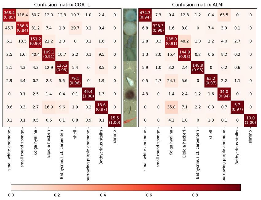
Sensors 2021, 21, 1134 3 of 16
years, convolutional neural networks have been successfully proposed as a very powerful
approach to computer vision problems, making the selection and tuning of classic hand
crafted features like dominant colors obsolete.
In this paper, we propose ALMI, a new active learning method for the object classifica-
tion in marine images using a generic deep learning feature representation. ALMI takes
sub-images, referred to as image patches in the following, and returns for each patch a
class label, describing its content. ALMI is built on two conceptual ideas: First, it combines
uncertainty sampling with relevance sampling to automatically select the next sample to
be classified by domain experts and added to the training set. Second, it achieves a new
level of flexibility by employing deep learning features instead of hand-crafted features
like dominant colors (see above) proposed in prior works.
We use two different data sets from marine imaging to demonstrate our method and
evaluate its performance in comparison with other methods. The two data sets differ
regarding the location and water depth where they were recorded, and consequently
regarding the taxonomic composition of species they contain. Moreover, the images from
one data set were taken from a cabled fixed underwater observatory (FUO) while the
images from the other data set were taken from a moving towed ocean floor observation
system (OFOS). Our experiments show that our method is able to perform well on image
sets that differ in various aspects. In both data sets, our generic approach outperforms the
state-of-the-art methods without any extensive tuning towards the individual data set.
The data sets used as input for ALMI in our experiments are explained in more detail
in the next section. Section 3 describes the proposed method ALMI, and the results of
the evaluation are given in Section 4. Section 5 will discuss the evaluation and wrap our
findings up.
2. Materials
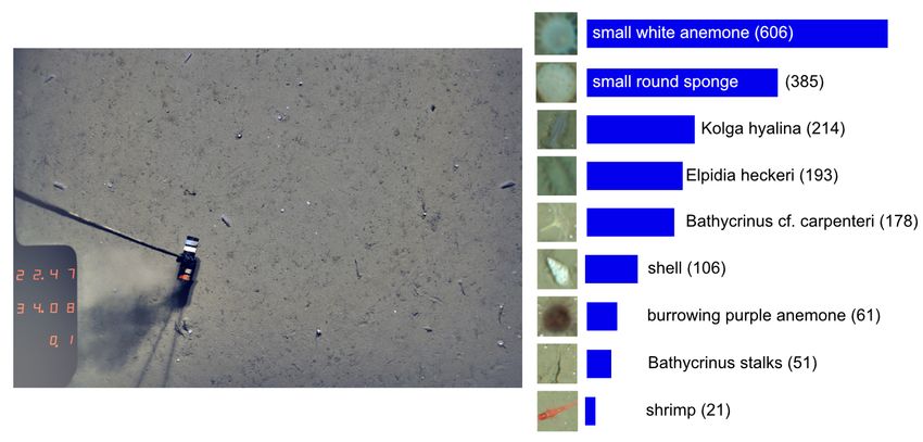
The first data set (see Figure 1) was created from an open-access, still image data set
taken at the Hausgarten observatory with an Ocean Floor Observation System (OFOS) [21,22].
The original images are publicly available as described in the Data Availability Statement
at the end of this paper. The Hausgarten observatory currently includes 21 stations located
between (N 78.5◦ , E 05◦ ) and (N 80◦ , E 11◦ ) between Greenland and Svalbard. The OFOS
was towed to a research vessel and took images of size 3504 × 2336 at a depth of 2500 m.
From the OFOS images, sub-images showing one object (like a sea star or a crustacean for
instance) were extracted by the authors of [6]. The resulting data set will be referred to as
Hausgarten dataset (HG). The dataset HG was used in [6] to evaluate the COATL learning
architecture and will be used in our experiments in Section 4.1. The HG data set used in
this work contains 1815 image patches grouped into 9 classes.
The second data set (see one example image in Figure 2) was created using images
from the Lofoten-Vesterålen (LoVe) Ocean Observatory. The original images are publicly
available as described in the Data Availability Statement at the end of this paper. LoVe
is a cabled fixed underwater observatory located at (N 68◦ 54.4740 , E 15◦ 23.1450 ) in the
Norwegian Sea about 22 km offshore. The observatory monitors a coral reef at a depth of
about 260 m. Among other sensors, the observatory is equipped with a high-resolution
digital camera taking images of the coral reef. One image of size 5184 × 3456 pixels is
taken once per hour. The change detection method proposed in [16] was used to extract
sub-images containing at most one object per sub-image from 24 LoVe images in an
unsupervised fashion. The resulting dataset will be referred to as LoVe data set (LV). The
LoVe dataset was used in [7] to evaluate an active learning method and will be used in our
experiments in Section 4.2. The LV dataset used in this work contains 3031 image patches
grouped into 6 classes. It mainly consists of one image patch class “no object” showing no
objects of interest (see Figure 2 on the right).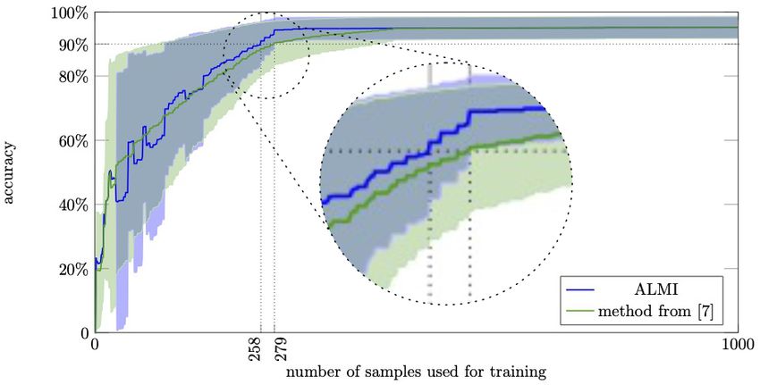
Sensors 2021, 21, 1134                                                                                                       4 of 16

      Figure 1. Images from the Hausgarten observatory (HG). Left: An original image. Right: The Hausgarten data set (HG) as
      used in experiments in Section 4.1. The numbers in brackets indicate the number of samples in a class. IMAGE: AWI OFOS
      team.

Figure 2. Images from the LoVe observatory. Left: An original image. Right: The LoVe data set (LV) as used in the experiments in
Section 4.2. The numbers in brackets indicate the number of samples in a class. The three dots indicate that the bar for the images
containing no object is out of scale for better visualization.

                                 3. Methods
                                       The proposed active learning workflow ALMI (see Figure 3) takes a set
                                I = { Ii | 1 ≤ i ≤ N } of images Ii (from here on, we will use the term image instead
                                of image patch) as input and assigns the images to classes that have a semantic meaning.
                                First, a fully automatic initialization step is performed to prepare the data for the semi-
                                automatic labeling process where semantic classes are found and training samples of all
                                classes are labeled and added to the training set. The initialization step starts by extracting
                                from each image Ii , a feature vector f i that represents the image in a lower-dimensional
                                (here 300 dimensional) vector space. Next, the feature vectors are grouped into M clusters
                                Cj , (1 ≤ j ≤ M) where features that are similar to each other belong to the same cluster. For
                                1 ≤ i ≤ N, we denote by ci the unique cluster index j with f i ∈ Cj . Moreover, a relevance
Sensors 2021, 21, 1134 5 of 16
score is computed for each cluster. This score estimates the potential of the cluster’s items
to improve the classifier’s learning performance in learning new classes not represented in
the training set (see Section 3.2 below).
li p
ro
el
ab
vid
labeling by
yl
e la
human expert
quer
bel li
relevance index
computation
full dataset
clustering classification
automated train the
feature extraction sample selection pro classifier
vid e u rtainty
nce
initialization
computer assisted labeling
Figure 3. Overview of the active learning method. In preparation for the selection of the training samples, the samples are
clustered, and a relevance index is assigned to each cluster. Furthermore, a feature vector is extracted for every image. For
the selection of the training images, three consecutive steps are repeated iteratively: (i) A training sample is chosen from the
set of images according to the sampling strategy and the state of the classifier. (ii) The sample is labeled by an expert. (iii)
The classifier is updated. The trained classifier can then be used to classify the remaining samples.
Next, the training set is composed, and in each iteration, the following three steps are
performed:
1. A sample image Ii is chosen automatically according to the sampling efficiency
criterion (defined below in the Sampling efficiency algorithm section)
2. An expert classifies the sample into a class found in a previous iteration or into a new
class.
3. The classifier is retrained to update the uncertainties used in the sampling criterion
(step 1).
The trained classifier can then be used to classify the remaining samples.
3.1. Feature Extraction
For further processing, for each image Ii , a feature vector f i is computed that describes
the image in a lower dimensional vector space. Due to the limited background knowl-
edge problem formulated in the introduction, the image feature representation cannot be
built with hand-crafted features using heuristics without a strong loss in generalization
(see Section 1). Instead, we propose to use the InceptionV3 Net [23], a fully convolutional
deep learning network, to extract features f i for any network input Ii . These features
however are abstract and are learned automatically during a pre-training step (see below).
A deep learning network takes the image Ii as input and passes it through a number
of so-called layers that transform the input and pass it to the next layer until the the image
is classified in the last layer. In the case of fully convolutional networks like InceptionV3,
the layers mainly consist of a number of filters. In the InceptionV3 Net (see Figure 4), the
layers are grouped into so-called inception modules inspired by the Inception Net described
in [24]. The inception modules take the output of the previous inception module as input (orSensors 2021, 21, 1134 6 of 16
the original image in case of the first inception module) and perform multiple convolutions
with different kernel sizes. The convolution results are then stacked on top of each other
and passed to the next inception module. The output of the last inception module can be
seen as a feature vector that is passed to the last layer for classification The filter-weights
are not predefined by human experts but are learned during the training, where images
are classified and the filter-weights are adjusted in an iterative process to optimize the
classification performance. In case of the InceptionV3 Net about 25 × 106 parameters
(mainly filter-weights) are learned during the training.
Figure 4. The InceptionV3 Net: Most layers of InceptionV3 are organized in so-called inception modules (see [23]). These
inception modules compute multiple convolutions that are concatenated and used as the output of the module. The output
of the last inception module before the classification layers (shaded gray) is used for feature extraction in our workflow.
To make sure that the filter-weights are set properly, we use an InceptionV3 Net
that was pretrained on a large set of images, the ImageNet [25]. ImageNet is a list of
web images that provides access to more than 14 × 106 annotated and quality-controlled
web images. The list includes images showing examples of a variety of concepts such as
sports, foot, animal, fish, etc. The subset of marine animals contains 1348 images. The
InceptionV3 Net pre-trained on the ImageNet data set used in this work was downloaded
using tensorflow [26].
To generate a feature vector f i for one images Ii , the images are fed into the pretrained
InceptionV3 Net and propagated through the layers. The output of the last layer of the
last inception module will be denoted by e f i . As these features e
f i are 2048-dimensional, we
reduce the dimension in order to enhance the computation time and performance of the
classifier. To do so, we use Principal Component Analysis (PCA) [27]. PCA is a method
for dimension reduction that can be thought of as understanding the feature vectors as
datapoint in the 2048-dimensional euclidean space and transforming them into a new
coordinate system that is determined in the following way. The first axis is determined to
minimize the sum of the squared distances between itself and each data point. The other
axes are determined one by one in the way that each axis minimizes the sum of squared
distances between itself and the data points under the condition of being orthogonal to
all previously determined axes. After transforming the feature vectors in this way, all but
the first 300 coordinates of each feature vector can be omitted without loosing too much
information (compare the explained variance in Sections 4.1 and 4.2). The feature vectors
obtained this way will be denoted by f i .
3.2. Cluster Relevance
The feature vectors are grouped into M clusters (i.e., groups of feature vectors that are
similar to one another) using a cluster method that takes the feature vectors as input and
returns for each feature vector f i a cluster index ci (1 ≤ ci ≤ M) as output. The choice of the
clustering method is not crucial in this context and is in general not dependent on the dataSensors 2021, 21, 1134 7 of 16
set or the kind of imaging setting. The method we use for the dataset HG is agglomerative
clustering. Agglomerative clustering starts with N clusters and assigns each feature vector
to its own cluster. Next, the number of clusters is reduced by iteratively choosing two
clusters according to a given criterion (here: wards criterion) and merge them until only m
clusters remain. Here, we use wards criterion that chooses the two clusters to be merged in
the way that the increase of the in-cluster variance is minimal.
In the case of the dataset LV, the images Ii were extracted automatically from larger
images using the change detection method BFCD [16] which only is applicable to images
from a fixed camera. In its core, BDFC extracts the images Ii containing maximum one
object per image as sub-images from a time-series of large scale images. This is done by
clustering the pixel-wise differences of the large scale images to the pixels of the mean
image of the large scale images. In that process not only the images Ii are returned but also
a cluster index ci (1 ≤ i ≤ M) for each image is returned, so no additional clustering is
required for the dataset LV.
For both data sets, the relevance scores of the clusters are computed as follows. For a
cluster j (1 ≤ j ≤ M), let
S j = { f i | 1 ≤ i ≤ N ∧ ci = j } (1)
denote the set of feature vectors that belong to cluster j and let
1
mj =
Sj
· ∑ fi (2)
f i ∈S j
denote the centroid of cluster j. With the mean of all feature vectors
1 N
N i∑
C= · fi (3)
=1
and the Euclidean distance d2 , the relevance score r j of cluster j is defined as the distance
r j = d2 C , m j (4)
between the centroid of cluster j and the mean of all feature vectors.
3.3. Sampling Efficiency Algorithm
Motivated by the criteria (a–d) defined in the introduction, we implement a sampling
algorithm to select the next training sample in two steps:
Step 1—Cluster selection: For selecting, a cluster, let the activity score a j denote the num-
ber of times a sample has been selected from cluster j in the previous iterations. By
defining
∞ if a j = 0
(
xj = rj (5)
a else
j
and selecting the cluster
ej = arg max( x j ) (6)
j
it is ensured that the frequency that a sample is drawn from cluster j is approximately
proportional to r j .
Step 2—Training sample selection: Let {ω1 , . . . , ωK(T) } denote the K (T ) classes that are
present in the training set during the sample selection in iteration t. If K (T ) ≥ 2,
uncertainty sampling [18] is used to draw a sample from the cluster ej selected in
step 1: Given a sample f i to be classified, a chosen classifier (e.g., the support vectorSensors 2021, 21, 1134 8 of 16
machine (SVM) [28] that is used in the experiments in this paper) computes for each
class ωk the probability pi,k (1 ≤ k ≤ K (T ) ) that f i belongs to ωk . With
(
(t) 1 if sample i has been labeled before iteration t
δi = (7)
0 else
the characteristic function that indicates if a sample has been labeled in an iteration
t0 < t, the uncertainty of the classifier regarding the classification of a feature f i can
then be expressed as
(t)
0 δi =1
ui = (8)
1 − max ( pi,k ) else
1≤ k ≤ K ( T )
To select the sample where the classifier is most uncertain, the sample fei with
ei = arg max ui (9)
{1≤i ≤ N | ci =ej}
is selected. In case K (T ) < 2, a classifier can not be trained and a sample is drawn
randomly with uniform distribution from the cluster ej selected in step 1.
3.4. Classification Uncertainty
As a last step in each iteration, the classifier has to be trained to obtain the uncertainties
that are used in the next iteration. In the t-th iteration, a number of t samples have been
labeled by the expert. The labels of the labeled samples are propagated to the remaining
samples using the clusters found in Section 3.2. To each cluster j, the label lˆj is assigned
that occurs most often in cluster j, according to
(t)
lˆj = arg max({1 ≤ i ≤ N | δi = 1 ∧ ci = j ∧ li = ωk }) (10)
1≤ k ≤ K ( T )
The labels assigned to the clusters are then used to assign a label to each sample,
according to
(t)
(
l if δi = 1
li = i
e (11)
lˆci else
The features f i and their labels e li are then used to train the classifier. The trained
classifier is then used to predict for each sample f i and each class ωk the probability pi,k
(1 ≤ j ≤ K (T ) ) that f i belongs to ωk . These probabilities are then used in the next iteration
to compute the uncertainties during the selection of the next sample.
4. Evaluation
ALMI is evaluated on the LoVe dataset and the Hausgarten dataset. The real-life
application with the human expert iteratively labeling the data as described above is
simulated with the data sets LV and HG that have been entirely labeled with gold standard
classifications gi by domain experts in advance. During each iteration, when the label for
an image Ii is queried, the a priori determined label gi is assigned to Ii . As a classifier, the
Support Vector Machine [28] (SVM) is used. The main idea of the SVM for two classes
is to find a hypersurface that separates the classes in the training set. To do so, the SVM
transform the samples into a higher-dimensional vector space until a separating hyperplane
can be found. The samples and the hyperplane are then transformed back to the original
vector space ending up with a hypersurface that separates the training data. A new sample
can then be classified by determining on which side of the hypersurface the sample is
located.Sensors 2021, 21, 1134 9 of 16
For each of the data sets, published results of a state-of-the-art method are available
for comparison. Each of these methods adds the training samples one by one in an
iterative fashion to the training data set similar to the iterations of the computer-assisted
labeling described in Sections 3.3 and 3.4. Atnthe end ofoeach iteration t, the classification
performance is evaluated on a test set T = Ii , . . . , Ii
1
⊂ I with the number N b of test
N
b
samples as described in the following two subsections.
To compute a classifier’s performance on T , let giτ denote the gold standard label
(t)
assigned to image Iiτ ∈ T by human experts. Furthermore, let hiτ denote the label assigned
to feature f iτ by the classifier when trained with t training samples. An often-used method
to evaluate a classifier’s performance is to compute the accuracy defined by
1 n b | h ( t ) = gi
o
a(t) = 1≤τ≤N iτ (12)
|T | τ
which describes the proportion of correctly classified samples in all classified samples.
However, for a fair evaluation of the methods on the LoVe dataset and the Hausgarten
dataset this performance measure will be changed slightly to match the evaluation in [6]
and [7] as described in the following two subsections.
4.1. Evaluation on the Dataset HG
In this experiment, the proposed method is evaluated on the dataset HG. First, the
result of the principal component analysis is inspected. As described in Section 3.1, the
PCA is used to reduce the InceptionV3 Net features from a length of 2048 to a length of
300. For this dataset, the explained variance of the first 300 principal components was
determined to be 94.2%. Next, the proposed method is compared to the COATL-approach
proposed in [6]. The core idea of COATL is to use different classifiers depending on the
number of available expert labels. No classifications are made until five labels are available.
From five to 20 available labels, a K-Nearest-Neighbors approach is used. From 20 to
400 labels, an SVM is used. From 400 to 1500 labels, an H2SOL [6] is used. Moreover, when
more than 1500 labels are available, a convolutional neural network is used.
As proposed in [6], after each iteration t, the performance is evaluated on all samples
except for the t labeled samples. By doing so, the test data set consists of N − t images after
iteration t. To avoid testing on a too small test dataset, only 1500 iterations are performed
which leaves 315 test samples after the last iteration. In both methods COATL and ALMI,
a number of nk first classifications are neglected. In case of COATL, this number is set to
nk = 5. In case of ALMI, all image classifications are neglected before more than one class
has been learned, i.e., K (T ) > 1 with K (T ) as the number of classes learned after T iterations.
That is why a slight modification of the accuracy given in Equation (12) is used in this
experiment.
n o
(t)
(
1
× 1 ≤ i ≤ N | h = g ∧ δ (t) = 0 if t ≥ 5 ∧ K (T ) ≥ 2
i
atHG = N −t i
(13)
0 else
The accuracy atHG is computed for the proposed method and for COATL after each
iteration. That is done 10 times for each method, and the average accuracies for each
method and each number of samples t are shown in Figure 5.Sensors 2021, 21, 1134 10 of 16
80%
75%
60%
accuracy
40%
20%
ALMI
COATL
0
0 68 150 454 750 1000
number of samples used for training
Figure 5. The accuracy values according to Equation (13) for ALMI (blue) and COATL (green) achieved on the Hausgarten
dataset. The vertical straight lines show how many labels are required to achieve a performance of 75% resp. 80%.
The results show that our new proposed generic method shows a steeper learning
rate than COATL, even without any particular tuning for this data. To achieve an accuracy
of 75%, the proposed method just needs 68 labels (4.5% of the training data), while COATL
needs 1023 labels (68.2% of the training data). An accuracy of 80% is achieved by the
proposed method with 150 labels (10% of the training data), while COATL does not achieve
an accuracy of 80%.
After 150 iterations when ALMI has an accuracy of 80.0%, the accuracy of COATL is
69.9%. To show which species are effected, the confusion matrix of COATL and ALMI after
150 iterations is shown in Figure 6.
The rows represent the true labels while the columns represent the predicted labels,
i.e., the number in row ι column κ represents how often an instance of class ι has been
predicted as class κ in average over the 10 runs. The numbers in brackets on the main
diagonal show the class-wise accuracies and have been computed as follows. For a class ι
let
• TPι denote the number of instances of class ι that have been correctly classified as
class ι,
• TNι denote the number of instances of any class κ 6= ι that have not been classified as
class ι,
• FPι denote the number of instances of any class κ 6= ι that have incorrectly been
classified as class ι, and
• FNι denote the number of instances of class ι that have been incorrectly classified as
class κ 6= ι.
The accuracy of class ι is then defined as
TPι + TNι
a(ι) = (14)
TPι + TNι + FPι + FNιSensors 2021, 21, 1134 11 of 16
Figure 6. Left: confusion matrix of COATL after 150 iterations. Right: confusion matrix of ALMI after 150 iterations. The
ι-th row of a matrix shows in the κ-th column how often an instance of class ι has been labeled as κ. The number in brackets
in a cell (ι, ι) represent the class-wise accuracy obtained by the classifier for class ι according to Equation (14). The color of a
cell (ι, ι) encodes the class-wise accuracy of class ι according to the color bar on the bottom. The colors in the other cells
(ι, κ ) represent the fraction of the number in (ι, κ ) in the sum of all numbers in the ι-th row or κ-th cell.
On the first glance, the class-wise accuracies obtained by the proposed method ALMI
seem to be better or equal to the class-wise accuracies obtained by COATL except for the
class “burrowing purple anemone”. In fact, also for the class “shrimp” COATL performs
a little better, as ALMI has more false negatives than COATL. That is not reflected by the
accuracy as the number of true negatives is quite high compared to the number of false
negatives for this underrepresented class leading to a accuracy of >0.95 for both methods.
As the overall accuracy shows, ALMI still outperforms COATL. As can be seen in the
upper right triangles of the confusion matrices, this is mainly due to fact that ALMI fixes
the problem that COATL tends to assign species incorrectly to more abundant classes.
4.2. Evaluation on the Data Set LV
In this experiment, ALMI is evaluated on the dataset LV. First, the feature vectors are
inspected. As described in Section 3.1, the InceptionV3 Net features are reduced from a
length of 2048 to a length of 300 using principal component analysis. For this dataset, the
explained variance of the first 300 principal components was determined to be 95.6%.Sensors 2021, 21, 1134 12 of 16
Next, ALMI is compared to the active learning approach based on dominant color
features, described in [7]. As in [7], 200 runs of the experiment have been conducted. Both
ALMI and the method described in [7] do not classify any sample before the number K
of classes in the training set exceeds 1. Several data-specific aspects had to be considered
in this evaluation. First, the test dataset is not strictly separated from the training dataset
and the classification performance is evaluated after each iteration on the whole dataset
including the labeled training data. Second, the expert labels available after t iterations are
included in the evaluation. To do so, let for 1 ≤ i ≤ N
(
( t ) li if δi = 1
hi =
b
(t) (15)
hi else
denote the labels that are used to train the classifier.
Third, to take the strong data imbalance and the dominating abundance of images
with no objects (see Figure 2 top right) into account, the performance measurement had to
be adapted. Otherwise, the performance measurement would easily measure very high
accuracies even for a naive classifier, classifying all images to the no object class. Thus,
to neglect the correctly classified no object-samples in the HG experiments the following
changes were applied to the number of images considered in the evaluation
n o
b = 1≤i≤N | ¬ b (t)
N h i = 0 ∧ gi = 0 (16)
and to the performance measure
( n o
t,r
1
hit = gi ∧ b
× 1≤i≤N | b hit 6= 0 if K (T ) ≥ 2
a LV = N b
(17)
0 else
The accuracy at,rLV is computed for ALMI and COATL after each iteration t. The
superscripts t and r denote here that the accuracy at,r
LV has been measured in the r-th run of
the experiment in iteration t (i.e., with t labeled samples). Along with the mean, Figure 7
shows the standard deviations computed and visualized as follows. With
1 200 t,r
200 r∑
µt = a LV (18)
=0
denoting the mean of the accuracy at iteration t averaged over all runs of the experiment,
the standard deviation of the accuracies after iteration t is defined as
v
u 200
σ = t ∑ (µt − at,r
u
t 2
LV ) (19)
r =0
The area between the curves of µt − σt and µt + σt is then filled with a semi-transparent
color.
Figure 7 shows that also on this dataset the results of ALMI outperform previously
published results on the same dataset. To achieve an accuracy of 90%, ALMI needs
258 labels (8.5% of the dataset), while the method in [7] needs 279 labels (9.2% of the
dataset). When the method in [7] achieves 90% accuracy, ALMI has already reached 94%
accuracy. In other words, ALMI has about 40% fewer misclassifications when trained with
279 labels. Regarding the standard deviation, the plot shows two things. First, after about
110 iterations, the accuracies achieved by ALMI vary less than the accuracies achieve by the
method proposed in [7]. Second, when the method proposed in [7] reaches an accuracy of
0.9%, the mean accuracy of ALMI is about one time the standard deviation larger than 0.9.Sensors 2021, 21, 1134 13 of 16
Figure 7. The accuracy values according to Equation (17) for ALMI (blue) and the method proposed in [7] (green) achieved
on the dataset LV. The blue and green areas visualize the standard deviation as computed in Equation (19). The circle shows
a magnification of the plots in the region around the 90% accuracy mark. The vertical straight lines show how many labels
are required to achieve a performance of 90%.
To test these findings about improving accuracy for statistical significance, we apply
two tests in order to check whether the variance and/or the mean of the accuracy obtained
after 279 iterations differs significantly depending on whether ALMI or the reference
method from [7] is used. For this, let A = ( a279,1 279,200
LV , . . . , a LV ) denote the accuracy values
obtained by ALMI after 279 iterations and let B = (bLV , . . . , b279,200
279,1
LV ) denote the according
accuracy values obtained by the method proposed in [7]. As a first test, we use the Levene
test [29] to test if the variances of A and B differ significantly. In the Levene test, the null
hypothesis states that the variances of A and B are equal. Next, a p-value is computed that
describes the probability that the variances of A and B differ more or equal than the actually
observed variances under the assumption of the null hypotheses. In our experiment, the
Levene test results in a p-value of about 3 × 10⁻⁹ . This is by far smaller than the typically
chosen threshold of 0.05 which shows that the null hypothesis should be rejected and the
difference of variances is highly significant. As a second test, we apply a one-sided Welch’s
test [30] to test if the mean of A is significantly larger than the mean of B. In the one-sided
Welch’s test, the null hypothesis states that the mean of A is lower or equal than the mean
of B. Next, a p-value is computed that describes the probability that mean( A) − mean( B)
is larger or equal than the actually observed difference between the means of A and B
under the assumption of the null hypothesis. In our experiment, the Levene test results
in a p-value of about 3 × 10⁻¹² . This is by far smaller than the typically chosen threshold
of 0.05 which shows that the null hypothesis should be rejected and the difference of the
accuracies is highly significant.
5. Discussion and Conclusions
The aim of this work was to present a generic method for marine image classification
that shows an improved learning performance due to the use of generic features and
a reasoned choice of training samples in order to increase the efficiency of the manual
annotation task performed by human experts. The proposed method ALMI is a single
label-image classification method, i.e., the images of the processed dataset are required
to contain maximum one object per image. However, if that is not the case, single-object
images can be extracted from large scale images prior to using ALMI fully automatic. SomeSensors 2021, 21, 1134 14 of 16
methods are proposed in [14–16] where the method proposed in [16] expects images from
fixed cameras. The other two methods can be applied to any kind of dataset, e.g., image
from OFOSs, FUOs, or semi-mobile platforms such as pan/tilt units.
To evaluate the extent to which the method meets this objective, its performance was
compared to other related works. The evaluation focused on several aspects. First, the
method was evaluated on very disparate data sets in order to assess the effectivity of the
generic feature approach. Second, results from previously published evaluations of existing
methods on the same data sets had to be available so results can be reproduced. Third, the
evaluation was done in the same way as the previously published evaluations in order
to visualize the progress. Regarding the evaluation in Section 4.2, one may observe that
the data was not split into test set and training set, which is of course common practice.
However, in active learning, it makes sense to leave the training data in the test set to avoid
a decrease of the test set’s quality. The decrease of the test set’s quality is more prominent
in a setup where object classes are underrepresented, and the true positive non-object
samples are not considered in the accuracy: As discussed above, an important feature of a
good sampling strategy is to draw samples from (potentially underrepresented) classes
that contain actual objects of interest. If these samples are removed from the test set, the
test set’s quality decreases faster with a “good” sampling strategy than with a strategy
that draws many “no object” samples. This is especially illustrated by the following two
points, which become only apparent when the training data are removed from the test set
and become apparent more quickly with a good sampling strategy than with a sampling
strategy that selects many “no object” samples.
1. When all the samples of an underrepresented class are in the training set, the under-
represented class is not part of the test set anymore.
2. When all the samples that are not in the “no object” class are in the training set, the
accuracy is 0 because the test set only contains “no object” images that are not counted
as true positives.
In our experiments on two data sets that use the same evaluation and the same data
set selected by the authors of the previously published method, ALMI shows that
1. it can achieve higher accuracies than previously published methods and
2. it has a steeper learning curve than, i.e., ALMI achieves a certain level of accuracy
with less training samples.
These effects are more prominent on the data set HG and are especially remarkable on
the data set LV, because on this data set the previously published method outperformed
the results of other known methods to such an extent that further improvement seemed
difficult to achieve. Considering the large differences between the two marine image data
sets, this all suggests that ALMI has the potential to apply to a wide range of marine image
data sets and makes us confident that it can be useful in the biodiversity estimation in
different types of marine habitats.
Author Contributions: T.M. and T.W.N.: Conceptualization, methodology, validation, formal anal-
ysis, investigation, data curation, writing–review and editing, visualization, and resources; T.M.:
software and writing–original draft preparation; T.W.N.: supervision, project administration, and
funding acquisition; All authors have read and agreed to the published version of the manuscript.
Funding: This work has been funded by the Bundesministerium für Wirtschaft und Energie (BMWI,
FKZ 0324254D) and financially supported through Equinor Contract No. 4590165310. The authors
would like to thank Equinor for the financial support and for providing field images.
Data Availability Statement: Links to the orignal Hausgarten images described in Section 2 para-
graph 1 can be downloaded at https://doi.pangaea.de/10.1594/PANGAEA.615724?format=textfile
(Last accessed on 30. December 2020). The original LoVe images described in Section 2 paragraph 2
are available under https://love.equinor.com/ (Last accessed on 30. December 2020).
Conflicts of Interest: The authors declare no conflicts of interest.Sensors 2021, 21, 1134 15 of 16
References
1. Bicknell, A.W.; Godley, B.J.; Sheehan, E.V.; Votier, S.C.; Witt, M.J. Camera technology for monitoring marine biodiversity and
human impact. Front. Ecol. Environ. 2016, 14, 424–432. [CrossRef]
2. Aguzzi, J.; Chatzievangelou, D.; Thomsen, L.; Marini, S.; Bonofiglio, F.; Juanes, F.; Rountree, R.; Berry, A.; Chumbinho, R.;
Lordan, C.; et al. The potential of video imagery from worldwide cabled observatory networks to provide information supporting
fish-stock and biodiversity assessment. ICES J. Mar. Sci. 2020, 77. [CrossRef]
3. Schoening, T.; Bergmann, M.; Ontrup, J.; Taylor, J.; Dannheim, J.; Gutt, J.; Purser, A.; Nattkemper, T.W. Semi-Automated Image
Analysis for the Assessment of Megafaunal Densities at the Arctic Deep-Sea Observatory HAUSGARTEN. PLoS ONE 2012,
7, e38179, [CrossRef] [PubMed]
4. Godø, O.R.; Johnson, S.; Torkelsen, T. The LoVe Ocean Observatory is in Operation. Mar. Technol. Soc. J. 2014, 48. [CrossRef]
5. Piepenburg, D.; Buschmann, A.; Driemel, A.; Grobe, H.; Gutt, J.; Schumacher, S.; Segelken-Voigt, A.; Sieger, R. Seabed images
from Southern Ocean shelf regions off the northern Antarctic Peninsula and in the southeastern Weddell Sea. Earth Syst. Sci. Data
2017, 9, 461–469. [CrossRef]
6. Langenkämper, D.; Nattkemper, T.W. COATL—A learning architecture for online real-time detection and classification assistance
for environmental data. In Proceedings of the 2016 23rd International Conference on Pattern Recognition (ICPR), Cancun, Mexico,
4–8 December 2016; pp. 597–602. [CrossRef]
7. Möller, T.; Nilssen, I.; Nattkemper, T.W. Active Learning for the Classification of Species in Underwater Images From a Fixed
Observatory. In Proceedings of the IEEE International Conference on Computer Vision (ICCV) Workshops, Venice, Italy, 22–29
October 2017.
8. Knapik, M.; Cyganek, B. Evaluation of Deep Learning Strategies for Underwater Object Search. In Proceedings of the 2019 First
International Conference on Societal Automation (SA), Krakow, Poland, 4–6 September 2019; pp. 1–6. [CrossRef]
9. Zurowietz, M.; Langenkämper, D.; Hosking, B.; Ruhl, H.A.; Nattkemper, T.W. MAIA—A machine learning assisted image
annotation method for environmental monitoring and exploration. PLoS ONE 2018, 13, e0207498, [CrossRef] [PubMed]
10. Liu, X.; Jia, Z.; Hou, X.; Fu, M.; Ma, L.; Sun, Q. Real-time Marine Animal Images Classification by Embedded System Based on
Mobilenet and Transfer Learning. In Proceedings of the OCEANS 2019, Marseille, France, 17–20 June 2019; pp. 1–5. [CrossRef]
11. Moniruzzaman, M.; Islam, S.; Bennamoun, M.; Lavery, P. Deep Learning on Underwater Marine Object Detection: A Survey.
In Advanced Concepts for Intelligent Vision Systems (ACIVS); Springer: Berlin/Heidelberg, Germany, 2017; pp. 150–160. [CrossRef]
12. Li, X.; Shang, M.; Qin, H.; Chen, L. Fast accurate fish detection and recognition of underwater images with Fast R-CNN. In
Proceedings of the OCEANS 2015—MTS/IEEE, Washington, DC, USA, 19–22 October 2015; pp. 1–5. [CrossRef]
13. Langenkämper, D.; Zurowietz, M.; Schoening, T.; Nattkemper, T.W. BIIGLE 2.0—Browsing and Annotating Large Marine Image
Collections. Front. Mar. Sci. 2017, 4, 83. [CrossRef]
14. Cho, M.; Kwak, S.; Schmid, C.; Ponce, J. Unsupervised Object Discovery and Localization in the Wild: Part-based Matching with
Bottom-up Region Proposals. In Proceedings of the IEEE Conference on Computer Vision and Pattern Recognition, Boston, MA,
USA, 7–12 June 2015.
15. Zhang, R.; Huang, Y.; Pu, M.; Zhang, J.; Guan, Q.; Zou, Q.; Ling, H. Object Discovery From a Single Unlabeled Image by Mining
Frequent Itemset With Multi-scale Features. arXiv 2020, arXiv:1902.09968.
16. Möller, T.; Nilssen, I.; Nattkemper, T.W. Change Detection in Marine Observatory Image Streams using Bi-Domain Feature
Clustering. In Proceedings of the International Conference on Pattern Recognition (ICPR 2016), Cancun, Mexico, 4–8 December
2016.
17. Langenkämper, D.; Simon-Lledó, E.; Hosking, B.; Jones, D.O.B.; Nattkemper, T.W. On the impact of Citizen Science-derived data
quality on deep learning based classification in marine images. PLoS ONE 2019, 14, e0218086. [CrossRef] [PubMed]
18. Settles, B. Active Learning Literature Survey; University of Wisconsin, Madison, WA, USA, 2010; Volume 52, p. 11.
19. Nguyen, H.T.; Smeulders, A. Active Learning Using Pre-clustering. In Proceedings of the Twenty-First International Conference
on Machine Learning (ICML 2004), Banff, Canada 4–8 July 2004; ACM: New York, NY, USA, 2004; p. 79. [CrossRef]
20. Fredrick, S.M. Quantization of Color Images Using the Modified Median Cut Algorithm. Ph.D. Thesis, Virginia Tech, Blacksburg,
VA, USA 1992.
21. Schewe, I.; Soltwedel, T. Sea-Bed Photographs (Benthos) from the AWI-Hausgarten Area Along OFOS Profile PS66/120-1. Ber. zur
Polar und Meeresforsch. Rep. Polar Mar. Res. 2007, 544, 242. [CrossRef]
22. Bergmann, M.; Klages, M. Increase of litter at the Arctic deep-sea observatory HAUSGARTEN. Mar. Pollut. Bull. 2012,
64, 2734–2741. [CrossRef] [PubMed]
23. Szegedy, C.; Vanhoucke, V.; Ioffe, S.; Shlens, J.; Wojna, Z. Rethinking the Inception Architecture for Computer Vision. In Proceed-
ings of the IEEE Conference on Computer Vision and Pattern Recognition (CVPR), Las Vegas, NV, USA, 27–30 June 2016.
24. Szegedy, C.; Wei Liu.; Yangqing Jia.; Sermanet, P.; Reed, S.; Anguelov, D.; Erhan, D.; Vanhoucke, V.; Rabinovich, A. Going deeper
with convolutions. In Proceedings of the 2015 IEEE Conference on Computer Vision and Pattern Recognition (CVPR), Boston,
MA, USA, 7–12 June 2015; pp. 1–9. [CrossRef]
25. Deng, J.; Dong, W.; Socher, R.; Li, L.J.; Li, K.; Li, F.-F. ImageNet: A Large-Scale Hierarchical Image Database. In Proceedings of
the 2009 IEEE Conference on Computer Vision and Pattern Recognition, Miami, FL, USA, 20–25 June 2009.
26. Abadi, M.; Agarwal, A.; Barham, P.; Brevdo, E.; Chen, Z.; Citro, C.; Corrado, G.S.; Davis, A.; Dean, J.; Devin, M.; et al. TensorFlow:
Large-Scale Machine Learning on Heterogeneous Systems; Software; 2015. Available online: tensorflow.org (accessed on 15. July 2019).Sensors 2021, 21, 1134 16 of 16
27. Pearson, K. LIII. On lines and planes of closest fit to systems of points in space. Lond. Edinb. Dublin Philos. Mag. J. Sci. 1901,
2, 559–572. [CrossRef]
28. Cortes, C.; Vapnik, V. Support-vector networks. Mach. Learn. 1995, 20, 273–297. [CrossRef]
29. Glass, G.V. Testing homogeneity of variances. Am. Educ. Res. J. 1966, 3, 187–190. [CrossRef]
30. Welch, B.L. The Generalization of ‘Student’s’ Problem when Several Different Population Variances are Involved. Biometrika 1947,
34, 28–35. [CrossRef] [PubMed]You can also read