Using the residual bootstrap to quantify uncertainty in mean apparent propagator MRI - bioRxiv
←
→
Page content transcription
If your browser does not render page correctly, please read the page content below

bioRxiv preprint first posted online Apr. 6, 2018; doi: http://dx.doi.org/10.1101/295667. The copyright holder for this preprint (which was not
                    peer-reviewed) is the author/funder. It is made available under a CC-BY-NC 4.0 International license.

                             Using the residual bootstrap to quantify
                          uncertainty in mean apparent propagator MRI

                          Xuan Gu1,3 , Anders Eklund1,2,3 , Evren Özarslan1,3 , and Hans Knutsson1,3
                      1
                          Division of Medical Informatics, Department of Biomedical Engineering, Linköping
                                                     University, Linköping, Sweden
                           2
                              Division of Statistics and Machine Learning, Department of Computer and
                                   Information Science, Linköping University, Linköping, Sweden
                            3
                              Center for Medical Image Science and Visualization, Linköping University,
                                                          Linköping, Sweden

                              Abstract. Estimation of noise-induced variability in MAP-MRI is needed
                              to properly characterize the amount of uncertainty in quantities derived
                              from the estimated MAP-MRI coefficients. Bootstrap metrics, such as the
                              standard deviation, provides additional valuable diffusion information in
                              addition to common MAP-MRI parameters, and can be incorporated in
                              MAP-MRI studies to provide more extensive insight. To the best of our
                              knowledge, this is the first paper to study the uncertainty of MAP-MRI
                              derived metrics. The noise variability of quantities of MAP-MRI have
                              been quantified using the residual bootstrap, in which the residuals are
                              resampled using two sampling schemes. The residual bootstrap method
                              can provide empirical distributions for MAP-MRI derived quantities,
                              even when the exact distributions are not easily derived. The residual
                              bootstrap methods are applied to SPARC data and HCP-MGH data,
                              and empirical distributions are obtained for the zero-displacement prob-
                              abilities. Here, we compare and contrast the residual bootstrap schemes
                              using all shells and within the same shell. We show that residual resam-
                              pling within each shell generates larger uncertainty than using all shells
                              for the HCP-MGH data. Standard deviation and quartile coefficient maps
                              of the estimated variability are provided.

                              Keywords: Bootstrap, Diffusion MRI, MAP-MRI, Uncertainty

                      1     Introduction

                      Mean apparent propagator (MAP) MRI is a diffusion-weighted MRI framework
                      for accurately characterizing and quantifying anisotropic diffusion properties at
                      large as well as small levels of diffusion sensitivity (Özarslan et al., 2013). Conse-
                      quently, it has been demonstrated that MAP-MRI can capture intrinsic nervous
                      tissue features (Avram et al., 2016; Fick et al., 2016; Özarslan et al., 2013). Some
                      novel features of the diffusion can be characterized by MAP-MRI, including the
                      return-to-origin probability (RTOP), return-to-plane probability (RTPP), and
                      the return-to-axis probability (RTAP). With the assumptions that the gradients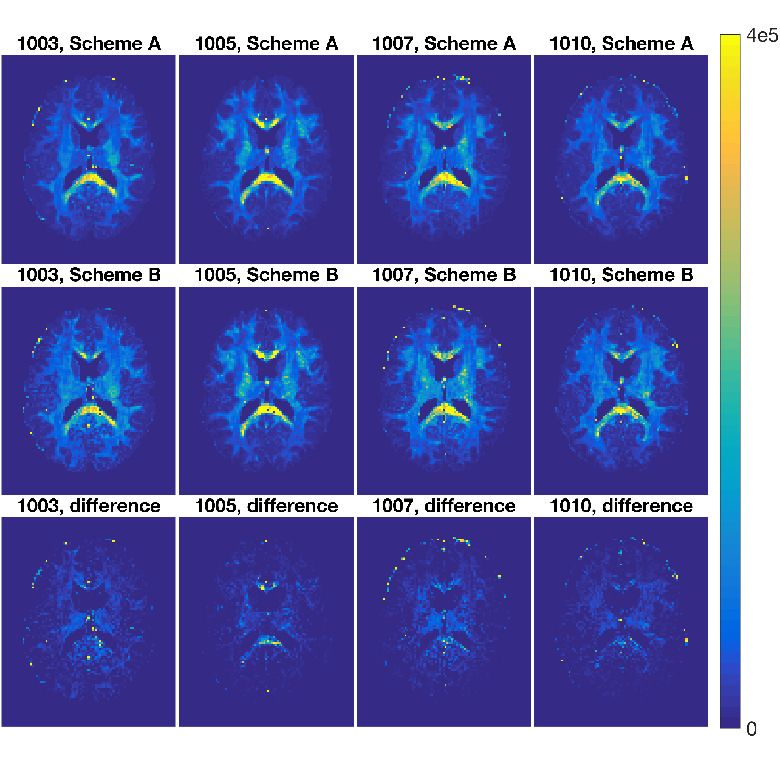
bioRxiv preprint first posted online Apr. 6, 2018; doi: http://dx.doi.org/10.1101/295667. The copyright holder for this preprint (which was not
                    peer-reviewed) is the author/funder. It is made available under a CC-BY-NC 4.0 International license.

                      are infinitely short and the diffusion time is sufficiently long, these MAP-MRI
                      derived metrics describe the mean pore volume and cross-sectional area for a
                      population of isolated pores. It is, however, not clear how high the uncertainty
                      is for these measures.

                          Bootstrap is a non-parametric statistical technique, based on data resam-
                      pling, used to quantify uncertainties of parameters (Efron, 1992). Bootstrap
                      has been widely used in diffusion tensor imaging (DTI) to study uncertainty
                      associated with DTI parameter estimation (Chung et al., 2006; Heim et al.,
                      2004; Pajevic and Basser, 2003; Vorburger et al., 2016, 2012; Yuan et al., 2008).
                      The repetition bootstrap method requires multiple measurements per gradient
                      direction to perform resampling (Heim et al., 2004). For most clinical and re-
                      search applications, it is more interesting to obtain more gradient directions,
                      since diffusion parameter estimation can be more robust with high angular res-
                      olution diffusion imaging (HARDI). To be able to use bootstrap for diffusion
                      data with multi gradient directions, instead of repetitions of the same direction,
                      residual bootstrap can be used with the assumption that the error terms have
                      constant variance. The wild bootstrap (Wu, 1986) is suited when the data are
                      heteroscedastic (i.e., non-constant variance). The sensitivity of the MAP-MRI
                      metrics on noise, experimental design, and the estimation of the scaling tensor
                      has been investigated in (Hutchinson et al., 2017).

                          Implementation of the repetition bootstrap, residual bootstrap and wild
                      bootstrap have already been reported for DTI (Chung et al., 2006; Efron, 1992;
                      Heim et al., 2004; Vorburger et al., 2016, 2012; Yuan et al., 2008) while there
                      are no reports of bootstrap for MAP-MRI. A possible explanation is the higher
                      computational complexity of MAP-MRI. The explanation is that DTI has been
                      used for a long time, while MAP-MRI is a rather new framework. We use a
                      model-based resampling technique, the residual bootstrap, that may be applied
                      to the residuals from the linear regression model used to fit MAP-MRI in each
                      voxel. The residual bootstrap is specifically designed to work when data are
                      homoscedastic; that is, when the variance of the errors is constant for all ob-
                      servations. For the standard diffusion tensor model the non-constant variance
                      comes from the log-transform of the diffusion signal, but no log-transform is
                      applied in MAP-MRI.

                         This paper investigates the ability of model-based resampling, in particular,
                      the residual bootstrap, to provide reasonable estimates of variability for MAP-
                      MRI derived quantities for physical phantom data (SPARC) (Ning et al., 2015)
                      and for human brain data (HCP-MGH) (Van Essen et al., 2013). Two sampling
                      schemes, residual sampling using all shells and within each shell, are used to
                      produce uncertainty maps. Comparisons are made between the two sampling
                      schemes, between data with different b-values, and also for different healthy
                      subjects. To the best of our knowledge, this is the first paper to study the
                      uncertainty of MAP-MRI derived metrics.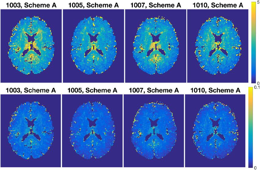
bioRxiv preprint first posted online Apr. 6, 2018; doi: http://dx.doi.org/10.1101/295667. The copyright holder for this preprint (which was not
peer-reviewed) is the author/funder. It is made available under a CC-BY-NC 4.0 International license.
2 Theory
2.1 MAP-MRI
The three-dimensional q-space diffusion signal attenuation E(q) is expressed in
MAP-MRI as
N
X max X
E(q) = an1 n2 n3 Φn1 n2 n3 (A, q), (1)
N =0 {n1 ,n2 ,n3 }
where Φn1 n2 n3 (A, q) are related to Hermite basis functions and depend on the
second-order tensor A and the q-space vector q. The non-negative indices ni are
the order of Hermite basis functions which satisfy the condition n1 +n2 +n3 = N .
The q-space vector q is defined as q = γδG/2π, where γ is the gyromagnetic
ratio, δ is the diffusion gradient duration, and G determines the gradient strength
and direction. The propagator is the three-dimensional inverse Fourier transform
of E(q), and can be expressed as
N
Xmax X
P (r) = an1 n2 n3 Ψn1 n2 n3 (A, r), (2)
N =0 {n1 ,n2 ,n3 }
where Ψn1 n2 n3 (A, r) are the corresponding basis functions in displacement space
r. The number of coefficients for MAP-MRI is given by
1 Nmax Nmax
Ncoef = b c+1 b + 2c . (3)
6 2 2
A can be taken to be the covariance matrix of displacement, defined as
2
ux 0 0
A = 2RT DRtd = 0 u2y 0 , (4)
0 0 u2z
where R is the transformation matrix whose columns are the eigenvectors of the
standard diffusion tensor D, and td is the diffusion time. The MAP-MRI basis
functions, Φn1 n2 n3 (A, q) in q-space and Ψn1 n2 n3 (A, r) in displacement r-space,
are given by
Φn1 n2 n3 (A, q) = φn1 (ux , qx )φn2 (uy , qy )φn3 (uz , qz ), (5)
Ψn1 n2 n3 (A, q) = ψn1 (ux , x)ψn2 (uy , y)ψn3 (uz , z), (6)
with (Özarslan et al., 2008)
i−n −2 2 2 2
φn (u, q) = √ e π q u Hn (2πuq), (7)
2n n!
1 2 2
ψ( n, x) = √ e−x /2u Hn (x/u), (8)
2n+1 πn!u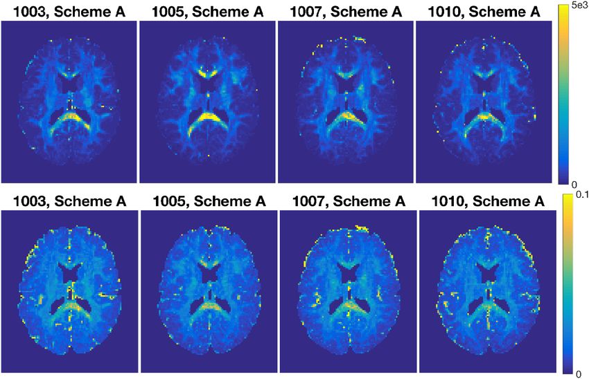
bioRxiv preprint first posted online Apr. 6, 2018; doi: http://dx.doi.org/10.1101/295667. The copyright holder for this preprint (which was not
                    peer-reviewed) is the author/funder. It is made available under a CC-BY-NC 4.0 International license.

                      where Hn (x) is the nth order Hermite polynomial. Equation 1 can be written in
                      matrix form as
                                                                  y = Qa + ε ,                                                 (9)
                      where y is a vector of T signal values, Q is a T × Ncoef design matrix formed by
                      the basis functions Φn1 n2 n3 (A, q), a contains the parameters to estimate, and ε
                      is the error. The coefficients a can be obtained by solving the following quadratic
                      minimization problem,
                                               min ||y − Qa||2 , Ka ≥ 0, 1T Ka ≤ 0.5,                                         (10)
                                                 a

                      where 0 and 1 are vectors with elements 0 and 1, respectively. The rows of
                      the constraint matrix K are the basis functions Ψn1 n2 n3 (A, q) evaluated on a
                      uniform Cartesian grid in the positive z half space. The first constraint enforces
                      non-negativity of the propagator, and the second one limits the integral of the
                      probability density to a value no greater than 1.
                          Zero displacement probabilities include the return-to-origin probability (RTOP),
                      and its variants in 1D and 2D: the return-to-plane probability (RTPP), and the
                      return-to-axis probability (RTAP), respectively. Return-to-origin-probability, P (r),
                      is the probability for water molecules to undergo no net displacement. In terms
                      of MAP-MRI coefficients through the expression it is defined as
                                                     N max
                                             1       X       X
                                   RT OP = p                         (−1)N/2 an1 n2 n3 Bn1 n2 n3 ,                            (11)
                                            8π 3 |A| N =0 {n ,n ,n }
                                                                          1       2     3

                      where
                                                                                       (n1 !n2 !n3 !)1/2
                                                     Bn1 n2 n3 = Kn1 n2 n3                               ,                    (12)
                                                                                        n1 !!n2 !!n3 !!
                      and Kn1 n2 n3 = 1 if n1 , n2 and n3 are all even and 0 otherwise. If we consider a
                      population of isolated pores, with the assumptions that the diffusion gradients
                      are infinitesimally short and the diffusion time is sufficiently long, it can be
                      shown that (Özarslan et al., 2013)
                                                             < V >= RT OP −1 ,                                                (13)
                      which indicates that the reciprocal of the RTOP is the statistical mean pore
                      volume.
                         RTAP indicates the probability density for molecules to return to the axis
                      determined by the principal eigenvector of the A-matrix. On the other hand,
                      RTPP represents the likelihood for no net displacement along this axis. If the
                      principal eigenvector is along the x-axis, RTAP and RTPP are given by
                                                      Nmax
                                                1     X               X
                                 RT AP =                                              (−1)(n2 +n3 )/2 an1 n2 n3 Bn1 n2 n3 ,   (14)
                                              2πuy uz
                                                          N =0 {n1 ,n2 ,n3 }
                                                     N max
                                                 1   X       X
                                 RT P P = √                          (−1)n1 /2 an1 n2 n3 Bn1 n2 n3 .                          (15)
                                                2πux N =0 {n ,n ,n }
                                                                  1   2       3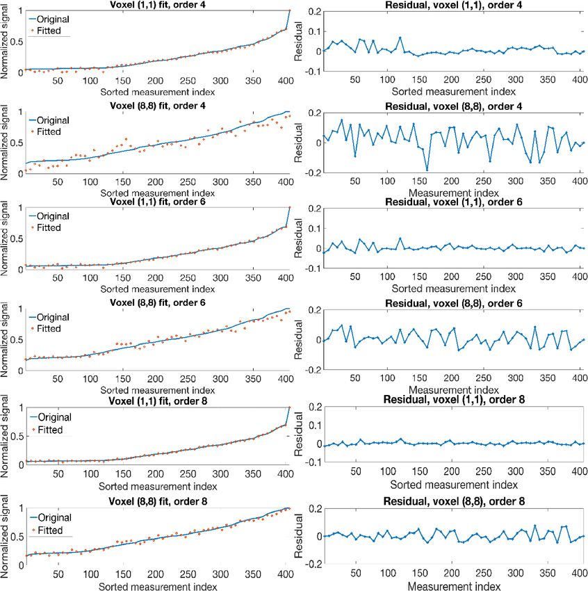
bioRxiv preprint first posted online Apr. 6, 2018; doi: http://dx.doi.org/10.1101/295667. The copyright holder for this preprint (which was not
                    peer-reviewed) is the author/funder. It is made available under a CC-BY-NC 4.0 International license.

                      2.2    Bootstrap
                      Repetition (regular) bootstrap requires multiple measurements per gradient di-
                      rection, and for each gradient direction the measurements are sampled with
                      replacement over-and-over again to characterize the uncertainty of the diffusion
                      derived metrics (Heim et al., 2004). However, nowadays it becomes clinically
                      more feasible to have scan protocols with a large number of gradient directions,
                      instead of having more than one measurement per direction.
                          Alternatives to repetition bootstrap are model-based bootstrap approaches,
                      such as the residual bootstrap and the wild bootstrap. Residual bootstrap relies
                      on the assumption that the residuals are independent and identically distributed
                      (e.g. constant variance); the sample diffusion data are generated by randomly
                      sampling with replacement from the residuals. Wild bootstrap is designed for
                      heteroscedastic data, that is when the variance of the errors is not constant. In
                      the case of the diffusion tensor model(Basser et al., 1994), it is known that the
                      log-transform leads to non-constant variance (Wegmann et al., 2017). Therefore,
                      the residuals are weighted by the heteroscedasticity consistent covariance ma-
                      trix estimator and random samples are drawn from the auxiliary distribution
                      (Davidson and Flachaire, 2008).
                          Under the assumption that ε is a vector of independent and identically dis-
                      tributed (IID) values with zero mean, the linear regression would be termed
                      homoscedastic and we would be able to randomly sample with replacement from
                      the residual, taking the form

                                                    yi∗ = (Qâ)i,· + ε∗i , i = 1, · · · , T,                         (16)

                      where (Qâ)i,· is the ith row of the product of Q and â, â is the solution of the
                      quadratic minimization problem in Equation 10, and ε∗i is a random sample from
                      the residuals of the original regression model ε̂ε = y − Qâ. The mean squared
                      error (MSE) can be used to quantify the quality of the signal reconstruction,
                      according to
                                                                           T
                                                                        1X 2
                                                             M SE =          ε̂ .                                    (17)
                                                                        T i=1 i

                        A common test for heteroscedasticity is the White test (White, 1980). A
                      White test can be performed using a second regression, according to

                                                          ε̂ε2 = δ0 + δ1 ŷ + δ2 ŷ2 ,                               (18)

                      where ŷ is the predicted diffusion signal. It is known that a higher b-value will
                      result in diffusion data with a lower signal-to-noise-ratio (SNR). It has been
                      reported that the SNR issue becomes important at higher b-values, when fitting
                      the data to a diffusion model (Gu et al., 2017). Hence it is more reasonable to
                      resample the residuals from the same b-value group (diffusion shell). We will
                      refer the bootstrap scheme as Scheme A when sampling using all shells, and
                      Scheme B when sampling within each shell separately.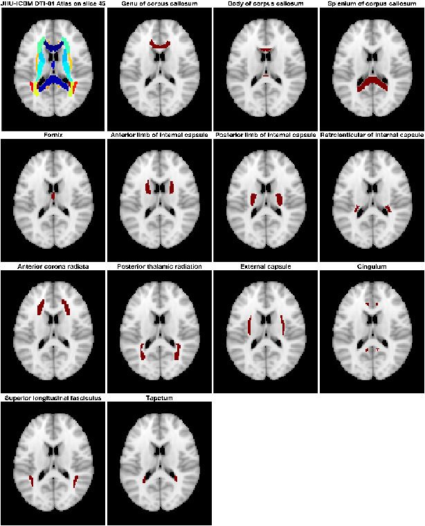
bioRxiv preprint first posted online Apr. 6, 2018; doi: http://dx.doi.org/10.1101/295667. The copyright holder for this preprint (which was not
                    peer-reviewed) is the author/funder. It is made available under a CC-BY-NC 4.0 International license.

                           Solving the quadratic minimization problem for y∗ = [y1∗ , · · · , yT∗ ] will pro-
                      duce a bootstrap estimate of the coefficients a∗ . Repeating these steps for some
                      fixed large number NB , resampling and estimation, builds up a collection of co-
                      efficients a∗1 , · · · , a∗NB called the bootstrap distribution, from which some MAP-
                      MRI scalar indices can be calculated. Summary statistics from this empirical
                      distribution can be used to describe the original parameter estimate. Here the
                      sample statistic θ̂ is an estimate of the true unknown θ (such as the noise-free
                      RTOP of the voxel) using the original data y, and θ̂∗ is the bootstrap replica-
                      tion of θ̂. The bootstrap-estimated standard error of θ̂ is simply the standard
                      deviation of the NB replications, i.e.,
                                                       v
                                                       u             NB h             i2
                                                       u        1    X
                                                 SDθ = t                  θ̂∗ (n) − µθ ,                             (19)
                                                              NB − 1 n=1

                                       PNB ∗
                      where µθ = N1B n=1     θ̂ (n). The Quartile coefficient (QC) is a dimensionless
                      measure of dispersion which can be computed using the first (Q1) and third
                      (Q3) quartiles (Bonett, 2006), according to

                                                                       Q3 − Q1
                                                              QC =             .                                     (20)
                                                                       Q3 + Q1

                      In this paper we use QC for comparing the dispersion of parameters.

                      3     Data and Methods

                      3.1    SPARC phantom data

                      We use data from the Sparse Reconstruction Challenge for Diffusion MRI (SPARC
                      dMRI) hosted at the 2014 CDMRI workshop on computational diffusion MRI
                      (Ning et al., 2015). The data were acquired from a physical phantom with known
                      fiber configuration. The phantom is made of polyfil fibers of 15 µm diameter
                      (Moussavi-Biugui et al., 2011). It provides a mask to indicate the number of
                      fiber bundles crossing in each voxel. In two-fiber voxels, the fiber bundles are
                      crossing at a 45 degree angle with isotropic diffusion outside. The voxels that
                      are masked by 0 have no fibers and are not considered. Three sets of data are
                      acquired with b-values of 1000, 2000, and 3000 s/mm2 , using 20, 30 and 60 gra-
                      dient directions per shell for the three datasets respectively (hereinafter referred
                      to as SPARC-20, SPARC-30 and SPARC-60). The gold-standard data was ob-
                      tained by acquiring 81 gradient directions at b-values of 1000, 2000, 3000, 4000
                      and 5000 s/mm2 averaged over 10 repetitions, resulting in 405 measurements
                      (hereinafter referred to as SPARC-Gold). All datasets include one measurement
                      with b0 . The data has dimension 13 × 16 × 406 and resolution 2 × 2 × 7 mm. The
                      diffusion time and pulse separation time are δ = ∆ = 62ms.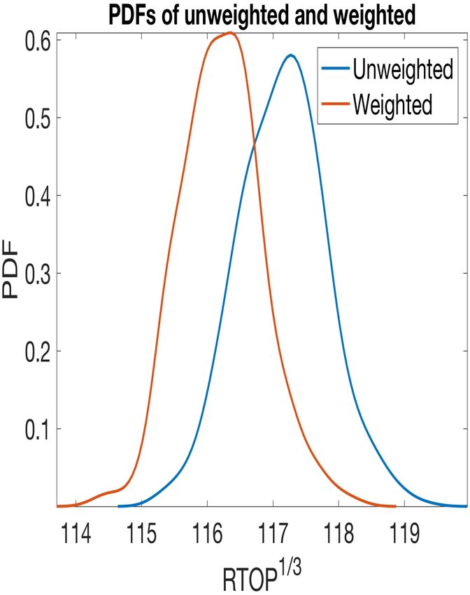
bioRxiv preprint first posted online Apr. 6, 2018; doi: http://dx.doi.org/10.1101/295667. The copyright holder for this preprint (which was not
                    peer-reviewed) is the author/funder. It is made available under a CC-BY-NC 4.0 International license.

                      3.2    Human Connectome Project MGH adult diffusion data

                      We use the MGH adult diffusion dataset from the Human Connectome Project
                      (HCP) (Van Essen et al., 2013). Data were collected from 35 healthy adults
                      scanned on a customized Siemens 3T Connectom scanner with 4 different b-
                      values (1000, 3000, 5000 and 10,000 s/mm2 ). The data has already been prepro-
                      cessed for gradient nonlinearity correction, motion correction and eddy current
                      correction (Glasser et al., 2013). The data consists of 40 non-diffusion weighted
                      volumes (b = 0), 64 volumes for b = 1000 and 3000 s/mm2 , 128 volumes for b =
                      5000 s/mm2 and 256 volumes for b = 10, 000 s/mm2 , which yields 552 volumes
                      of 140 × 140 × 96 voxels with an 1.5 mm isotropic voxel size. The diffusion time
                      and pulse separation time are δ = 12.9 ms and ∆ = 21.8 ms. The HCP-MGH
                      data also contains high-resolution T1 images of 256 × 256 × 276 voxels with an
                      1.0 mm isotropic voxel size.
                          Data used in the preparation of this work were obtained from the Human
                      Connectome Project (HCP) database (https://ida.loni.usc.edu/login.jsp). The
                      HCP project (Principal Investigators: Bruce Rosen, M.D., Ph.D., Martinos Cen-
                      ter at Massachusetts General Hospital; Arthur W. Toga, Ph.D., University of
                      Southern California, Van J. Weeden, MD, Martinos Center at Massachusetts
                      General Hospital) is supported by the National Institute of Dental and Cranio-
                      facial Research (NIDCR), the National Institute of Mental Health (NIMH) and
                      the National Institute of Neurological Disorders and Stroke (NINDS). HCP is
                      the result of efforts of co-investigators from the University of Southern Califor-
                      nia, Martinos Center for Biomedical Imaging at Massachusetts General Hospital
                      (MGH), Washington University, and the University of Minnesota.

                      3.3    Methods

                      Diffusion tensor fitting, MAP-MRI fitting and bootstrap sampling were imple-
                      mented using C++. The initial tensor fitting was performed with data with
                      b-values less than 2000 s/mm2 using weighted least squares. To impose the con-
                      straint of positivity of the propagator, we sample P (r) in a 21 × 21 × 11 grid,
                      resulting in 4851 points. Here the last dimension is only sampled on its positive
                      axis as the propagator is antipodally symmetric. We use the Gurobi Optimizer
                      (Gurobi Optimization, 2016) to solve the quadratic optimization problem. The
                      Open Multi-Processing (OpenMP) (Dagum and Menon, 1998) framework is used
                      to run the analysis for many voxels in parallel. MAP-MRI fitting and bootstrap
                      sampling are computationally expensive, due to the large number of MAP co-
                      efficients, constraints in the quadratic minimization problem and repeating the
                      analysis 500-5000 times. We use a computer with 512 GB RAM and two In-
                      tel(R) Xeon(R) E5-2697 2.30 GHz CPUs. Each of the two CPUs has 18 cores
                      (36 threads), which makes it possible to run the analysis for 72 voxels in parallel.
                           In order to perform a voxel-level group comparisons of diffusion-derived met-
                      ric maps, the diffusion data must be transformed to a standard space. The trans-
                      formation between MNI standard space and diffusion space is achieved in three
bioRxiv preprint first posted online Apr. 6, 2018; doi: http://dx.doi.org/10.1101/295667. The copyright holder for this preprint (which was not
peer-reviewed) is the author/funder. It is made available under a CC-BY-NC 4.0 International license.
separate steps. First, the non-diffusion volume is registered to the T1 volume us-
ing the FSL (Jenkinson et al., 2012) function epi reg. Second, the T1 volume is
non-linearly registered to the MNI152 T1 2mm template using the FSL function
fnirt (Andersson et al., 2007). Third, the two transformations were combined, to
transform the diffusion data to MNI space. The statistics analysis is performed
in MATLAB (R2016b, The MathWorks, Inc., Natick, Massachusetts, United
States).
4 Results
4.1 SPARC
Fig. 1. Top left: the fiber bundles mask, top right: Mean Diffusivity (MD) (mm2 /s),
bottom left: Fractional Anisotropy (FA), bottom right: RTOP1/3 (mm−1 ) for SPARC-
Gold. It can be seen that MD differs for different fiber configurations, while FA is more
or less constant in fibrous areas. The RTOP1/3 shows lower values in single-fiber areas,
but higher in two-fiber voxels.
Results of the SPARC-Gold data will be used as a comparison reference for
the following study on SPARC-20, SPARC-30 and SPARC-60. Figure 1 showsbioRxiv preprint first posted online Apr. 6, 2018; doi: http://dx.doi.org/10.1101/295667. The copyright holder for this preprint (which was not
peer-reviewed) is the author/funder. It is made available under a CC-BY-NC 4.0 International license.
scalar maps of the fiber bundles mask, fractional anisotropy (FA), mean diffu-
sivity (MD) and RTOP1/3 . The values in the fiber bundles mask indicate the
number of fiber bundles in each voxel. The voxels masked by 0 are referred as
empty area. The construction of the physical phantom is described in (Moussavi-
Biugui et al., 2011). The MD clearly shows different diffusivities in two-fiber areas
(4.78 ± 0.63 × 10⁻⁴ mm2 /s) and single-fiber areas (7.51 ± 0.67 × 10⁻⁴ mm2 /s). In
single-fiber and crossing-fiber areas the FA shows very similar values (0.82 ± 0.03
and 0.85 ± 0.01, respectively). Finally, for the Nmax of 6 for MAP-MRI, we find
fairly consistent RTOP1/3 values in both single-fiber (81.0 ± 7.87 m−1 ) and two-
fiber (111.7 ± 11.1 m−1 ) areas and higher in the two-fiber areas. Also, it can be
noticed that RTOP1/3 in two-fiber area shows a larger degree of variation (larger
standard deviation).
To study the effect of the MAP-MRI Nmax on signal reconstruction, we com-
pare the signal reconstruction quality over different Nmax s for SPARC-Gold.
Figure 2 shows the original diffusion signal, the MAP-MRI fitted signal and the
residuals for an unidirectional voxel (1,1) and a bidirectional voxel (8,8) from
SPARC-Gold. For comparison, we normalized the signal with the first volume
(b0 ) . For higher Nmax s both voxels have a lower error. There is a substantially
lower error in single-fiber voxels than two-fiber voxels. Larger Nmax s (more basis
functions) provide a better characterization of the diffusion signal. The amount
of additional detail in the reconstruction of the propagator does not increase be-
yond a certain point. The trade-off between the level of detail in the propagator
estimation, the amount of data acquired and the computation time is important.
It is reported that including terms up to order 6 was found to yield a sufficient
level of detail in propagators from diverse brain regions (Fick et al., 2016). In
this paper all further analysis of MAP-MRI parameters described in this paper
use Nmax = 8, if not specified otherwise.
To study the quality of the MAP-MRI signal fitting, we focus on two vox-
els; one unidirectional voxel (1,1) and one bidirectional voxel (8,8). The mean
squared error (MSE) and the computation time (using 30 CPU threads) of the
signal recovery for the two voxels is summarized in Figure 3. Please note that
the computation time plotted is for the SPARC-30 data, in order to compare
with the results in (Fick et al., 2016). It can be noted that the quality of sig-
nal fitting for the single-fiber voxel (1,1) quickly reaches the optimum when the
Nmax is larger than 4. For the two-fiber voxel (8,8), no substantial differences
in the signal fitting can be observed when the Nmax is beyond 6. The number
of MAP-MRI coefficients to be estimated in each voxel for the Nmax of 2 to 10
is 7, 22, 50, 95, 161, respectively. With the help of OpenMP and the Gurobi
Optimizer, we are able to perform the MAP-MRI fitting for SPARC-30 using a
Nmax of 10 within 15 seconds, which is 17 times faster than its counterpart in
(Fick et al., 2016).
Figure 4 show the standard deviation of RTOP1/3 for SPARC-20, SPARC-
30, SPARC-60 and SPARC-Gold, using the two bootstrap sampling schemes and
500 bootstrap samples. The standard deviation values are directly proportional
to the RTOP values. For all datasets the standard deviation maps exhibit minorbioRxiv preprint first posted online Apr. 6, 2018; doi: http://dx.doi.org/10.1101/295667. The copyright holder for this preprint (which was not
peer-reviewed) is the author/funder. It is made available under a CC-BY-NC 4.0 International license.
Fig. 2. Normalized diffusion signals, MAP-MRI fitted signals and residuals for
an unidirectional voxel (1,1) and a bidirectional voxel (8,8) from SPARC-Gold,
using Nmax 4, 6 and 8. Measurement indices are sorted in an ascending or-
der of the signal intensities. The 406 samples represent diffusion data from b =
0, 1000, 2000, 3000, 4000, 5000 mm2 /s
differences for the two sampling schemes. A reduction in the standard deviation
is observed with an increasing number of diffusion measurements and gradient
directions from SPARC20 to SPARC-Gold. This is explained by the fact that
the data acquisition protocols with a larger number of diffusion measurements
and gradient directions will improve the signal fitting quality, which reduces the
variability of the estimated RTOP values. As shown in Figure 5, it is notable
that the mean standard deviation of the two-fiber area demonstrates a downward
trend from SPARC-20 to SPARC-60, as the number of measurements increased
from 41 to 61 and 121, using the same gradient strength. With 406 measurementsbioRxiv preprint first posted online Apr. 6, 2018; doi: http://dx.doi.org/10.1101/295667. The copyright holder for this preprint (which was not
peer-reviewed) is the author/funder. It is made available under a CC-BY-NC 4.0 International license.
Fig. 3. Left: the mean squared error of the reconstructed signal with respect to the
diffusion signal for an unidirectional voxel(1,1) and a bidirectional voxel(8,8) from
SPARC-Gold. Right: the computation time in seconds for two implementations of
MAP-MRI.
Fig. 4. Standard deviation of the RTOP1/3 for SPARC-20, SPARC-30, SPARC-60 and
SPARC-Gold, using two bootstrap sampling schemes and 500 bootstrap samples. The
standard deviation is clearly lower for SPARC-Gold. Scheme A: sampling using all
shells, Scheme B: sampling within each shell.
and b-values of 1000 to 5000, the mean standard deviation of the two-fiber area
for SPARC-Gold is dramatically decreased. The single-fiber area is not affected
by the number of measurements.
Figure 6 shows the QC of the RTOP1/3 for SPARC-20, SPARC-30, SPARC-
60 and SPARC-Gold, using two bootstrap sampling schemes and 500 samples.
The mean quartile coefficients for SPARC-Gold show less variability, and this is
to be expected since SPARC-Gold is based on more gradient directions and more
measurements. We can see that one potential source of variability comes from
the bootstrap sampling methodology. Data with a larger number of gradient
directions produces more stable estimates of MAP-MRI coefficients, from which
RTOP is based. Scheme A and B for SPARC-Gold data produce similar estimates
of uncertainty. The QC maps from Scheme B show more smooth and consistentbioRxiv preprint first posted online Apr. 6, 2018; doi: http://dx.doi.org/10.1101/295667. The copyright holder for this preprint (which was not
peer-reviewed) is the author/funder. It is made available under a CC-BY-NC 4.0 International license.
Fig. 5. Mean standard deviation (left) and mean QC (right) of the RTOP1/3 for single-
fiber voxels and two-fiber voxels in SPARC-20, SPARC-30, SPARC-60 and SPARC-
Gold, using bootstrap Scheme A (sampling using all shells) and 500 samples.
Fig. 6. QC of the RTOP1/3 for SPARC-20, SPARC-30, SPARC-60 and SPARC-Gold,
using two bootstrap sampling schemes and 500 bootstrap samples. Scheme A: sampling
using all shells, Scheme B: sampling within each shell.
results for SPARC-20, SPARC-30 and SPARC-60. It is interesting to note that
the QC maps from all sampling schemes for SPARC-Gold are exhibiting larger
variability for single-fiber areas, compared to two-fiber areas.
Figure 7 shows the histograms of RTOP1/3 for SPARC-60 using one bootstrap
sample and 500 samples. The mean values for single-fiber and two-fiber areas
are plotted as vertical lines. With 500 samples, the histogram is able to reflect
the distribution in which two patterns can be detected, corresponding to the two
fiber configurations.
Figure 8 and 9 show the histograms of the RTOP1/3 of an unidirectional voxel
(1,1) and a bidirectional voxel (8,8) for SPARC-20, SPARC-30, SPARC-60 and
SPARC-Gold, using two bootstrap sampling schemes and 500 bootstrap samples.
It is interesting to note that the means of the RTOP1/3 of the unidirectional voxel
(1,1) are different for Scheme A and Scheme B.bioRxiv preprint first posted online Apr. 6, 2018; doi: http://dx.doi.org/10.1101/295667. The copyright holder for this preprint (which was not
peer-reviewed) is the author/funder. It is made available under a CC-BY-NC 4.0 International license.
Fig. 7. Histograms of the RTOP1/3 for all voxels in SPARC-60, using bootstrap Scheme
A (sampling using all shells) and 500 bootstrap samples.
Fig. 8. Histograms of the RTOP1/3 of an unidirectional voxel (1,1) for SPARC-20,
SPARC-30, SPARC-60 and SPARC-Gold, using two bootstrap sampling schemes and
500 bootstrap samples. Scheme A: sampling using all shells, Scheme B: sampling using
the same shell.
Figure 10 shows the PDF of the RTOP1/3 for SPARC-20, SPARC-30, SPARC-
60 and SPARC-Gold, using two bootstrap sampling schemes and 500 bootstrap
samples. The PDFs of RTOP1/3 for SPARC-20, SPARC-30 and SPARC-60 show
only minor differences between the two bootstrap sampling schemes since these
three datasets were acquired using the same b-values. Both bootstrap sampling
schemes show the ability to detect some patterns in the PDF of the RTOP1/3
corresponding to the two fiber configurations in the phantom, although with abioRxiv preprint first posted online Apr. 6, 2018; doi: http://dx.doi.org/10.1101/295667. The copyright holder for this preprint (which was not
peer-reviewed) is the author/funder. It is made available under a CC-BY-NC 4.0 International license.
Fig. 9. Histograms of the RTOP1/3 of a bidirectional voxel (8,8) for SPARC-20,
SPARC-30, SPARC-60 and SPARC-Gold, using two bootstrap sampling schemes and
500 bootstrap samples. Scheme A: sampling using all shells, Scheme B: sampling within
each shell.
Fig. 10. PDF of the RTOP1/3 for SPARC-Gold, SPARC-20, SPARC-30 and SPARC-
60, using two bootstrap sampling schemes and 500 bootstrap samples. Scheme A:
sampling using all shells, Scheme B: sampling within each shell.
few notable differences. The SPARC-Gold data does exhibit a different distribu-
tion when compared with the other three. It can be inferred that the bootstrap-
generated distributions might be related to the b-value settings used in the scans
but less affected by the number of measurements.
Figure 11 shows the boxplots of the RTOP1/3 for an unidirectional voxel
(1,1) and a bidirectional voxel (8,8) for SPARC-20, SPARC-30, SPARC-60 and
SPARC-Gold, using two bootstrap sampling schemes and 500 bootstrap sam-bioRxiv preprint first posted online Apr. 6, 2018; doi: http://dx.doi.org/10.1101/295667. The copyright holder for this preprint (which was not
peer-reviewed) is the author/funder. It is made available under a CC-BY-NC 4.0 International license.
Fig. 11. Boxplot of the RTOP1/3 for an unidirectional voxel (1,1) (top) and a bidirec-
tional voxel (8,8) (bottom) for SPARC-20, SPARC-30, SPARC-60 and SPARC-Gold,
using two bootstrap sampling schemes and 500 bootstrap samples. Scheme A: sampling
using all shells, Scheme B: sampling within each shell. The uncertainty is clearly lower
for SPARC-Gold
.bioRxiv preprint first posted online Apr. 6, 2018; doi: http://dx.doi.org/10.1101/295667. The copyright holder for this preprint (which was not
peer-reviewed) is the author/funder. It is made available under a CC-BY-NC 4.0 International license.
ples. On each box, the central mark indicates the median, and the bottom
and top edges of the box indicate the 25th and 75th percentiles Q1 and Q3 ,
respectively. The whiskers represent the ranges for the bottom and the top
boundaries of the data values, excluding outliers. The boundaries are calcu-
lated as Q3 − 1.5 × (Q3 –Q1 ) and Q3 + 1.5 × (Q3 –Q1 ) (McGill et al., 1978), which
corresponds to approximately 99.3 percent coverage if the data are normally
distributed. The outliers are plotted individually using the 0 +0 symbol beyond
the boundaries. Non-skewed data, with a median in the center, indicates that
data may be normally distributed. For both voxels, the RTOP distributions for
SPARC-20 exhibits a larger amount of variability. For a bidirectional voxel (8, 8),
the bootstrap samples of RTOP show much narrower distributions. The boxplots
of the RTOP1/3 indicate little difference in the two sampling schemes.
4.2 HCP-MGH
In the following section, we present results from HCP-MGH diffusion data.
White test Figure 12 shows examples of MD, FA and RTOP of a slice from
subject MGH-1010. Figure 13 shows the results from the White test for the
residuals from all shells, and within each shell. The first column demonstrates
that most voxels produce a p-value below 0.05 (uncorrected for multiple com-
parisons) which rejects the null hypothesis of homoskedasticity for the residuals
from all shells. Columns 2 to 5 show that 5.1%, 4.9%, 5.3% and 5.0% of the
voxels in the brain demonstrate heteroskedasticity, i.e. close to the expected 5%
if the null hypothesis is true. These tests show that sampling within each shell
should be used.
Fig. 12. MD, FA and RTOP for subject MGH-1010, slice 45.
Uncertainty of RTOP, RTAP and RTPP In Figure 14, the standard devi-
ation of RTOP for subjects MGH-1003, 1005, 1007 and 1010 are shown. TherebioRxiv preprint first posted online Apr. 6, 2018; doi: http://dx.doi.org/10.1101/295667. The copyright holder for this preprint (which was not
peer-reviewed) is the author/funder. It is made available under a CC-BY-NC 4.0 International license.
Fig. 13. Results from the White test (testing for heteroscedastic variance); for all shells
(column 1) and each shell separately (columns 2-5). R-squared values and voxels with a
p-value ¡ 0.05 (uncorrected for multiple comparisons) are shown for subject MGH-1010,
slice 45. The proportion of significant voxels in the brain mask are 5.1%, 4.9%, 5.3%
and 5.0% for columns 2-5, i.e. close to the expected 5% for a threshold of p = 0.05.
are two main clusters of voxels in the standard deviation maps wherein the white
matter areas generally appear hyperintense, while the gray matter areas make
up the lower intensity regions. There is limited contrast within the gray matter
areas because it is relatively isotropic. Within the white matter areas, a large
variability is detected in the corpus callosum areas for all four subjects. Within
the corpus callosum, the splenium part shows a larger standard deviation than
the genu and body of the corpus callosum.
Figure 15 shows the QC of RTOP for subjects MGH-1003, 1005, 1007 and
1010. The QC measures dispersion of the distribution for 500 bootstrap RTOP
samples without considering the RTOP values. Compared with the standard
deviation maps in Figure 14, it is obvious that the contrast between the white
matter and the gray matter decreases. A portion of the white matter regions
shows larger QC values, most notably in the splenium of the corpus callosum.
A larger dispersion is found in some gray matter voxels and this information
and contrast are not available in the corresponding standard deviation maps.
It is interesting to note the corpus callosum which has a highly anisotropic,
coherent single fiber architecture demonstrates a much larger variability than
other white matter areas. Figure 16 and 17 show the standard deviation and
QC of RTAP and RTPP for subjects MGH-1003, 1005, 1007 and 1010, using
bootstrap sampling Scheme A. Figure 18 shows the histograms of RTOP for a
GM voxel and a WM voxel from subjects MGH-1003, 1005, 1007 and 1010.
To study the uncertainty of diffusion metrics derived from MAP-MRI for
different white matter tracts, we summarize the mean standard deviation and
mean QC of RTOP for JHU ICBM-DTI-81 White-Matter Labels (Mori et al.,
2005) in Appendix Table 1, using bootstrap Scheme A and 500 bootstrap sam-bioRxiv preprint first posted online Apr. 6, 2018; doi: http://dx.doi.org/10.1101/295667. The copyright holder for this preprint (which was not
peer-reviewed) is the author/funder. It is made available under a CC-BY-NC 4.0 International license.
Fig. 14. First and second rows: standard deviation of RTOP for subjects MGH-1003,
1005, 1007, 1010, slice 45, using two bootstrap sampling schemes and 500 bootstrap
samples. Third row: absolute difference. Scheme A: sampling using all shells, Scheme
B: sampling within each shell.
ples. The JHU ICBM-DTI-81 White-Matter Labels are displayed in Figure 20.
Both the standard deviation and the QC in Appendix Table 1 emphasize that
the splenium of the corpus callosum exhibits relatively larger variability for the
500 bootstrap samples of RTOP, which is also accentuated in Figure 14 and 15.
Splenium is the thickest part of the corpus callosum which connects the poste-
rior cortices with fibers varying in size. For subjects 1003, 1005, and 1007, the
splenium of the corpus callosum produces the largest QC values, and for sub-
ject 1010 the fornix gives the largest uncertainty. The mean QC of the anterior
corona radiata tracts is substantially smaller than other labelled parts for all four
subjects. However, in the regions where fibers cross or merge and the anisotropy
becomes low, the uncertainty is seen to be high. Tractography results obtainedbioRxiv preprint first posted online Apr. 6, 2018; doi: http://dx.doi.org/10.1101/295667. The copyright holder for this preprint (which was not
peer-reviewed) is the author/funder. It is made available under a CC-BY-NC 4.0 International license.
Fig. 15. First and second rows: QC of RTOP for subjects MGH-1003, 1005, 1007, 1010,
slice 45, using two bootstrap sampling schemes and 500 bootstrap samples. Third row:
absolute difference. Scheme A: sampling using all shells, Scheme B: sampling within
each shell.
for tracts that pass through such regions are likely to be very irreproducible
and it would therefore be interesting to perform repeatability studies of tract
reconstructions using MAP-MRI for tracts in these regions.
Appendix Table 2 shows the mean standard deviation and mean QC of RTOP
for JHU ICBM-DTI-81 White-Matter Labels using bootstrap Scheme B and 500
bootstrap samples. It is notable that sampling residuals within each shell leads
to slightly larger variability for all JHU white matter tracts. Bootstrap sampling
serves primarily as a measure of precision for diffusion-derived metrics, so there is
the expected correlation with the SNR value. It is reported in (Vorburger et al.,
2016) that the dispersion of diffusion tensor principal eigenvector in fornix is
correlated with the subjects’ memory performance. As expected, the spleniumbioRxiv preprint first posted online Apr. 6, 2018; doi: http://dx.doi.org/10.1101/295667. The copyright holder for this preprint (which was not
peer-reviewed) is the author/funder. It is made available under a CC-BY-NC 4.0 International license.
Fig. 16. Std (top) and QC (below) of RTAP for subjects MGH-1003, 1005, 1007,
1010, slice 45, using bootstrap sampling Scheme A (sampling using all shells) and 500
bootstrap samples.
of the corpus callosum produces relatively larger standard deviation and QC
values, and for subjects 1003, 1007 and 1010, the fornix tract demonstrates the
largest variability. The anterior corona radiata tracts always produce the least
uncertainty, regardless of the bootstrap sampling schemes using all shells or
within the same shell.
Appendix Table 3 shows the mean QC of RTAP and RTPP for JHU ICBM-
DTI-81 White-Matter Labels using bootstrap Scheme A and 500 bootstrap sam-
ples. The best precision is achieved by the anterior corona radiata, followed by
superior long fasciculus for RTAP. Generally, the statistics of RTAP demon-
strates a similar behavior as RTOP. The RTPP and RTAP values can be seen
as the “decomposition” of the RTOP values into components parallel and per-
pendicular to the direction of the primary eigenvector of the diffusion tensor,
respectively. Generally, the variation pattern across the white matter tracts is
similar for all three investigated MAP-MRI metrics. In other words, if the uncer-
tainty in a white matter tract is high with respect to RTOP, it is also high with
respect to the other two parameters, i.e., RTAP and RTPP. Appendix Tables
1, 2 and 3 indicate that we should be less confident in the MAP-MRI derived
metrics from those tracts with relatively higher QC values.
Group analysis Similar to functional MRI it is common to perform group
studies using diffusion MRI, to for example find differences between healthybioRxiv preprint first posted online Apr. 6, 2018; doi: http://dx.doi.org/10.1101/295667. The copyright holder for this preprint (which was not
peer-reviewed) is the author/funder. It is made available under a CC-BY-NC 4.0 International license.
Fig. 17. Std (top) and QC (below) of RTPP for subjects MGH-1003, 1005, 1007,
1010, slice 45, using bootstrap sampling Scheme A (sampling using all shells) and 500
bootstrap samples.
controls and subjects with some disease. One of the most common scalar mea-
sures for group analysis is fractional anisotropy, calculated from the diffusion
tensor, which for example has been used to study diffuse axonal injuries in mild
traumatic brain injury (Eierud et al., 2014; Shenton et al., 2012). A weighted
mean can be calculated as
PN
n=1 (wn xn )
µ= P N
(21)
n=1 wn
where wn = 1/σn2 . Instead of each voxel value contributing equally to the final
mean, voxels with higher standard deviation contribute less “weight” than oth-
ers. A comparison between the mean RTOP and the weighted mean RTOP is
presented in Figure 19. The weighted mean for example downweights an outlier
close to the posterior cingulate. In Figure 19, it is also presented a comparison of
the unweighted and the weighted probability density distributions of RTOP1/3
for one voxel. Subjects with a higher uncertainty will be downweighted, which
can lead to a different distribution of the mean RTOP1/3 .
5 Discussion
Researchers have previously applied the bootstrap method to the residuals from
the linear regression used to fit the diffusion tensor model. We have extended thisbioRxiv preprint first posted online Apr. 6, 2018; doi: http://dx.doi.org/10.1101/295667. The copyright holder for this preprint (which was not
peer-reviewed) is the author/funder. It is made available under a CC-BY-NC 4.0 International license.
Fig. 18. Histograms of RTOP for a GM voxel and a WM voxel, subjects MGH-1003,
1005, 1007, 1010, slice 45, using bootstrap Scheme A (sampling using all shells) and
500 bootstrap samples.
Fig. 19. Mean and weighted mean of RTOP, PDFs of unweighted and weighted RTOP,
subjects MGH-1003, 1005, 1007, 1010, slice 45, using bootstrap Scheme A (sampling
using all shells) and 500 bootstrap samples.
technique to a more sophisticated diffusion model to quantify the uncertainty
of its derived metric. We used the residual bootstrap technique to evaluate the
uncertainty of the MAP-MRI derived metrics using physical phantom data as
well as human brain data. To the best of our knowledge, this is the first work
that investigates the uncertainty of diffusion metrics derived from MAP-MRI.
The experiments are divided into two sections: one dealing with uncertainty
estimation for physical phantom data in which four sets of data are collectedbioRxiv preprint first posted online Apr. 6, 2018; doi: http://dx.doi.org/10.1101/295667. The copyright holder for this preprint (which was not
peer-reviewed) is the author/funder. It is made available under a CC-BY-NC 4.0 International license.
using different number of measurements and different b-values, and the other
dealing with uncertainty estimation for human brain data of four healthy sub-
jects collected using the same scan protocol. The variability originates from mea-
surement noise and is influenced by a wide range of parameters, many of which
are difficult or impossible to fully model. It is generally assumed that diffusion
data are primarily affected by thermal, normally distributed noise. However,
physiological noise and artifacts may also affect diffusion data and may result in
non-normal and spatially variant noise characteristics.
Several studies report that for the diffusion tensor model, the variability
in the tensor trace, diffusion anisotropy, and the tensor major eigenvector are
related to the spatial orientation of the tensor (Batchelor et al., 2003; Jones and
Pierpaoli, 2004). The orientational dependence of the tensor variance decreases
for both more uniformly distributed encoding schemes and increased number of
encoding directions. In the experiment using SPARC data, we have demonstrated
that the variability of MAP-MRI derived metrics decrease for both increased
number of shells and increased number of gradient directions in each shell. The
variation in single-fiber area is less sensitive to the number of gradient directions
on each shell. A voxel with two fiber bundles and a voxel with a single fiber bundle
might lead to the same RTOP value, but the uncertainty might be affected
differently. It can be concluded that using a large number of shells is more
efficient to minimize the variation in the MAP-MRI diffusion metrics, compared
with a large number of measurements on the same shell.
Bootstrap Schemes A and B, sampling residuals using all shells and within
each shell, produce essentially identical results of standard deviation and QC
when applied to the SPARC data. This may be because that in the SPARC
data there is only one measurement for the shell b0 . It should be noted that
when using bootstrap Scheme B, that is sampling residuals within each shell, an
increased variability is found for MAP-MRI metrics in the HCP-MGH human
brain diffusion data (Figure 14 and 15) but is not found in the SPARC data.
The probability densities of RTOP were estimated to investigate configura-
tion of local diffusion profiles in the SPARC data. It is demonstrated that the
probability density follows expected patterns corresponding to the fiber configu-
rations in the physical phantom using both bootstrap sampling schemes. These
patterns do not differ much when the number of gradient directions on each shell
is changed, but provide more details when more shells are used in the diffusion
scan protocols.
It is important to note that all acquisition parameters which influence the
SNR of the diffusion signals, such as the b-value, the number of measurements,
the gradient strength, the echo time, etc., most likely have a direct influence on
the uncertainty.
In (Avram et al., 2016), the computation time for the reconstruction of MAP-
MRI parameters from whole-brain diffusion data sets (70 × 70 × 42 × 698) using
Nmax = 6 was less than 3 h on a single workstation with 32GB RAM and 8
cores (Intel i7-4770 K at 3.5G Hz). In (Fick et al., 2016), it is reported that it
takes around 60 seconds to do the MAP-MRI fitting (Nmax of 6) for all voxelsbioRxiv preprint first posted online Apr. 6, 2018; doi: http://dx.doi.org/10.1101/295667. The copyright holder for this preprint (which was not
peer-reviewed) is the author/funder. It is made available under a CC-BY-NC 4.0 International license.
of SPARC-30, using an Intel(R) Core(TM) i7-3840QM CPU with 32 GB RAM.
In this paper, we use two Intel(R) Xeon(R) E5-2697 CPUs and OpenMP to
support multi-thread processing, which makes it possible to do the MAP-MRI
fitting (Nmax of 6) for all voxels of SPARC-30 within 2 seconds. To run 500
bootstrap replicates takes about 40 minutes and 20 hours, respectively for the
SPARC data and a slice of the HCP-MGH data. In theory, graphics processing
units (GPUs) can be used for further speedup (Eklund et al., 2013, 2014) as they
can process some 30 000 voxels in parallel.
In conclusion, bootstrap metrics, such as the standard deviation and QC,
provide additional valuable diffusion information next to the common MAP-
MRI parameters and should be incorporated in ongoing and future MAP-MRI
studies to provide more extensive insight.
Acknowledgements
This research is supported by the Swedish Research Council (grant 2015-05356,
”Learning of sets of diffusion MRI sequences for optimal imaging of micro struc-
tures”), Linköping University Center for Industrial Information Technology (CENIIT),
and the Knut and Alice Wallenberg Foundation project “Seeing Organ Func-
tion”.
Data collection and sharing for this project is provided by the Human Con-
nectome Project (HCP; Principal Investigators: Bruce Rosen, M.D., Ph.D., Arthur
W. Toga, Ph.D., Van J. Weeden, MD). HCP funding was provided by the Na-
tional Institute of Dental and Craniofacial Research (NIDCR), the National
Institute of Mental Health (NIMH), and the National Institute of Neuro-logical
Disorders and Stroke (NINDS). HCP data are disseminated by the Laboratory
of Neuro Imaging at the University of Southern California.
A AppendixbioRxiv preprint first posted online Apr. 6, 2018; doi: http://dx.doi.org/10.1101/295667. The copyright holder for this preprint (which was not
peer-reviewed) is the author/funder. It is made available under a CC-BY-NC 4.0 International license.
Fig. 20. JHU-ICBM DTI-81 Atlas on slice 45.bioRxiv preprint first posted online Apr. 6, 2018; doi: http://dx.doi.org/10.1101/295667. The copyright holder for this preprint (which was not
peer-reviewed) is the author/funder. It is made available under a CC-BY-NC 4.0 International license.
Table 1. Mean std and QC of RTOP, JHU ICBM-DTI-81 White-Matter Labels, sub-
ject 1003, 1005, 1007 and 1010, slice 45, using bootstrap Scheme A (sampling using all
shells) and 500 bootstrap samples.
std (×104 /mm3 ) QC
Atlas Label Subjects Subjects
1003 1005 1007 1010 1003 1005 1007 1010
Genu of corpus callosum 7.34 16.0 11.1 9.45 0.0228 0.0328 0.0274 0.0255
Body of corpus callosum 10.9 20.0 15.9 11.4 0.0319 0.0410 0.0383 0.0315
Splenium of corpus callosum 23.7 25.0 24.6 20.2 0.0500 0.0477 0.0506 0.0425
Fornix 11.0 13.2 11.3 13.5 0.0488 0.0364 0.0396 0.0499
Anterior limb of internal capsule R 7.12 9.49 13.0 9.09 0.0211 0.0240 0.0303 0.0255
Anterior limb of internal capsule L 6.53 10.3 10.0 7.15 0.0212 0.0252 0.0260 0.0221
Posterior limb of internal capsule R 13.5 11.1 12.4 9.85 0.0344 0.0274 0.0312 0.0272
Posterior limb of internal capsule L 8.44 12.3 10.2 8.01 0.0275 0.0308 0.0300 0.0251
Retrolenticular part of internal capsule R 9.83 8.38 14.1 8.82 0.0308 0.0243 0.0352 0.0269
Retrolenticular part of internal capsule L 7.93 8.60 10.0 8.20 0.0274 0.0278 0.0296 0.0266
Anterior corona radiata R 3.60 5.69 5.09 4.73 0.0128 0.0161 0.0152 0.0147
Anterior corona radiata L 3.55 5.57 4.82 4.41 0.0129 0.0161 0.0144 0.0140
Posterior thalamic radiation R 7.89 4.49 5.86 6.91 0.0269 0.0173 0.0206 0.0228
Posterior thalamic radiation L 6.11 6.55 6.08 7.39 0.0237 0.0218 0.0219 0.0237
External capsule R 6.55 6.71 7.00 6.30 0.0205 0.0186 0.0200 0.0179
External capsule L 6.73 5.96 5.95 6.07 0.0234 0.0170 0.0189 0.0210
Cingulum R 5.89 8.02 7.99 7.28 0.0201 0.0218 0.0245 0.0217
Cingulum L 6.64 6.44 7.53 5.86 0.0229 0.0187 0.0233 0.0200
Superior longitudinal fasciculus R 7.59 5.29 5.84 5.31 0.0235 0.0165 0.0181 0.0176
Superior longitudinal fasciculus L 6.85 7.48 6.58 6.09 0.0228 0.0221 0.0203 0.0198
Tapetum R 5.14 4.62 5.67 3.95 0.0249 0.0216 0.0247 0.0209
Tapetum L 3.63 3.04 6.57 5.34 0.0205 0.0168 0.0241 0.0347
Table 2. Mean std and QC of RTOP, JHU ICBM-DTI-81 White-Matter Labels, sub-
ject 1003, 1005, 1007 and 1010, slice 45, using bootstrap Scheme B (sampling within
the shell) and 500 bootstrap samples.
std (×104 /mm3 ) QC
Atlas Label Subjects Subjects
1003 1005 1007 1010 1003 1005 1007 1010
Genu of corpus callosum 10.1 19.5 14.5 11.1 0.0317 0.0390 0.0350 0.0302
Body of corpus callosum 14.1 27.4 18.9 13.9 0.0408 0.0531 0.0429 0.0374
Splenium of corpus callosum 24.7 29.6 27.0 21.8 0.0586 0.0539 0.0575 0.0467
Fornix 12.4 14.9 17.2 20.6 0.0768 0.0389 0.0785 0.0805
Anterior limb of internal capsule R 8.61 11.3 15.2 10.4 0.0270 0.0284 0.0364 0.0310
Anterior limb of internal capsule L 8.38 12.9 12.5 8.92 0.0290 0.0314 0.0336 0.0295
Posterior limb of internal capsule R 15.1 13.5 15.2 13.4 0.0407 0.0335 0.0389 0.0370
Posterior limb of internal capsule L 10.4 15.4 11.9 9.62 0.0346 0.0385 0.0362 0.0308
Retrolenticular part of internal capsule R 10.8 10.5 17.2 11.1 0.0362 0.0305 0.0430 0.0357
Retrolenticular part of internal capsule L 10.8 9.89 11.3 8.83 0.0386 0.0333 0.0340 0.0294
Anterior corona radiata R 5.36 6.66 6.51 6.33 0.0193 0.0190 0.0197 0.0201
Anterior corona radiata L 5.61 6.89 6.18 5.89 0.0201 0.0201 0.0184 0.0190
Posterior thalamic radiation R 8.92 4.59 6.26 6.77 0.0326 0.0187 0.0232 0.0232
Posterior thalamic radiation L 6.61 6.85 6.92 8.01 0.0274 0.0229 0.0262 0.0267
External capsule R 8.62 7.64 8.70 8.36 0.0277 0.0211 0.0249 0.0252
External capsule L 8.48 7.29 8.34 7.92 0.0308 0.0207 0.0267 0.0283
Cingulum R 9.48 9.83 10.76 8.85 0.0342 0.0271 0.0339 0.0255
Cingulum L 10.1 7.75 8.95 7.55 0.0363 0.0228 0.0293 0.0253
Superior longitudinal fasciculus R 9.21 5.83 6.14 5.67 0.0308 0.0191 0.0198 0.0195
Superior longitudinal fasciculus L 7.69 7.35 7.47 5.94 0.0267 0.0223 0.0233 0.0200
Tapetum R 5.18 4.69 5.52 4.28 0.0264 0.0230 0.0260 0.0327
Tapetum L 4.09 2.63 7.25 7.52 0.0238 0.0156 0.0264 0.0597bioRxiv preprint first posted online Apr. 6, 2018; doi: http://dx.doi.org/10.1101/295667. The copyright holder for this preprint (which was not
peer-reviewed) is the author/funder. It is made available under a CC-BY-NC 4.0 International license.
Table 3. Mean QC of RTAP and RTPP, JHU ICBM-DTI-81 White-Matter Labels,
subject 1003, 1005, 1007 and 1010, slice 45, using bootstrap Scheme A (sampling using
all shells) and 500 bootstrap samples.
RTAP RTPP
Atlas Label Subjects Subjects
1003 1005 1007 1010 1003 1005 1007 1010
Genu of corpus callosum 0.0260 0.0329 0.0276 0.0275 0.0211 0.0158 0.0166 0.0173
Body of corpus callosum 0.0324 0.0388 0.0357 0.0305 0.0317 0.0235 0.0249 0.0253
Splenium of corpus callosum 0.0482 0.0432 0.0467 0.0396 0.0226 0.0190 0.0193 0.0182
Fornix 0.0567 0.0362 0.0617 0.0358 0.0461 0.0317 0.0425 0.0354
Anterior limb of internal capsule R 0.0267 0.0247 0.0308 0.0253 0.0181 0.0143 0.0154 0.0156
Anterior limb of internal capsule L 0.0256 0.0250 0.0276 0.0249 0.0184 0.0147 0.0165 0.0186
Posterior limb of internal capsule R 0.0330 0.0262 0.0298 0.0258 0.0168 0.0136 0.0152 0.0151
Posterior limb of internal capsule L 0.0285 0.0291 0.0287 0.0252 0.0179 0.0147 0.0167 0.0169
Retrolenticular part of internal capsule R 0.0299 0.0250 0.0347 0.0268 0.0198 0.0155 0.0174 0.0164
Retrolenticular part of internal capsule L 0.0285 0.0265 0.0284 0.0283 0.0186 0.0151 0.0157 0.0164
Anterior corona radiata R 0.0207 0.0199 0.0187 0.0191 0.0220 0.0151 0.0158 0.0166
Anterior corona radiata L 0.0197 0.0189 0.0195 0.0203 0.0210 0.0153 0.0176 0.0182
Posterior thalamic radiation R 0.0279 0.0178 0.0220 0.0232 0.0189 0.0144 0.0160 0.0141
Posterior thalamic radiation L 0.0262 0.0225 0.0247 0.0245 0.0220 0.0141 0.0172 0.0156
External capsule R 0.0244 0.0201 0.0214 0.0224 0.0187 0.0142 0.0151 0.0164
External capsule L 0.0263 0.0194 0.0218 0.0239 0.0181 0.0164 0.0173 0.0191
Cingulum R 0.0232 0.0248 0.0263 0.0234 0.0238 0.0162 0.0180 0.0170
Cingulum L 0.0266 0.0228 0.0250 0.0212 0.0200 0.0152 0.0180 0.0168
Superior longitudinal fasciculus R 0.0256 0.0197 0.0212 0.0201 0.0164 0.0146 0.0153 0.0146
Superior longitudinal fasciculus L 0.0248 0.0216 0.0214 0.0205 0.0171 0.0119 0.0142 0.0134
Tapetum R 0.0291 0.0232 0.0253 0.0333 0.0382 0.0347 0.0332 0.0262
Tapetum L 0.0250 0.0193 0.0250 0.0430 0.0385 0.0376 0.0298 0.0261bioRxiv preprint first posted online Apr. 6, 2018; doi: http://dx.doi.org/10.1101/295667. The copyright holder for this preprint (which was not
peer-reviewed) is the author/funder. It is made available under a CC-BY-NC 4.0 International license.
Bibliography
Andersson, J. L., Jenkinson, M., Smith, S., et al. (2007). Non-linear registration,
aka spatial normalisation fmrib technical report tr07ja2. FMRIB Analysis
Group of the University of Oxford, 2.
Avram, A. V., Sarlls, J. E., Barnett, A. S., Özarslan, E., Thomas, C., Irfanoglu,
M. O., Hutchinson, E., Pierpaoli, C., and Basser, P. J. (2016). Clinical feasi-
bility of using mean apparent propagator (MAP) MRI to characterize brain
tissue microstructure. NeuroImage, 127:422–434.
Basser, P. J., Mattiello, J., and LeBihan, D. (1994). Estimation of the effective
self-diffusion tensor from the nmr spin echo. Journal of Magnetic Resonance,
Series B, 103(3):247–254.
Batchelor, P., Atkinson, D., Hill, D., Calamante, F., and Connelly, A. (2003).
Anisotropic noise propagation in diffusion tensor mri sampling schemes. Mag-
netic Resonance in Medicine, 49(6):1143–1151.
Bonett, D. G. (2006). Confidence interval for a coefficient of quartile variation.
Computational Statistics & Data Analysis, 50(11):2953–2957.
Chung, S., Lu, Y., and Henry, R. G. (2006). Comparison of bootstrap approaches
for estimation of uncertainties of dti parameters. NeuroImage, 33(2):531–541.
Dagum, L. and Menon, R. (1998). Openmp: an industry standard api for shared-
memory programming. IEEE computational science and engineering, 5(1):46–
55.
Davidson, R. and Flachaire, E. (2008). The wild bootstrap, tamed at last.
Journal of Econometrics, 146(1):162–169.
Efron, B. (1992). Bootstrap methods: another look at the jackknife. In Break-
throughs in statistics, pages 569–593. Springer.
Eierud, C., Craddock, R. C., Fletcher, S., Aulakh, M., King-Casas, B., Kuehl, D.,
and LaConte, S. M. (2014). Neuroimaging after mild traumatic brain injury:
Review and meta-analysis. NeuroImage: Clinical, 4:283 – 294.
Eklund, A., Dufort, P., Forsberg, D., and LaConte, S. M. (2013). Medical image
processing on the GPU - Past, present and future. Medical Image Analysis,
17(8):1073 – 1094.
Eklund, A., Dufort, P., Villani, M., and LaConte, S. (2014). BROCCOLI: Soft-
ware for fast fMRI analysis on many-core CPUs and GPUs. Frontiers in
Neuroinformatics, 8:24.
Fick, R. H., Wassermann, D., Caruyer, E., and Deriche, R. (2016). MAPL:
Tissue microstructure estimation using Laplacian-regularized MAP-MRI and
its application to HCP data. NeuroImage, 134:365–385.
Glasser, M. F., Sotiropoulos, S. N., Wilson, J. A., Coalson, T. S., Fischl, B., An-
dersson, J. L., Xu, J., Jbabdi, S., Webster, M., Polimeni, J. R., et al. (2013).
The minimal preprocessing pipelines for the human connectome project. Neu-
roimage, 80:105–124.
Gu, X., Sidén, P., Wegmann, B., Eklund, A., Villani, M., and Knutsson, H.
(2017). Bayesian diffusion tensor estimation with spatial priors. In Inter-
national Conference on Computer Analysis of Images and Patterns, pages
372–383. Springer.You can also read