Assessing probabilistic modelling for wind speed from numerical weather prediction model and observation in the Arctic - Nature
←
→
Page content transcription
If your browser does not render page correctly, please read the page content below
www.nature.com/scientificreports
OPEN Assessing probabilistic modelling
for wind speed from numerical
weather prediction model
and observation in the Arctic
Hao Chen1*, Yngve Birkelund1, Stian Normann Anfinsen2, Reidar Staupe‑Delgado1 &
Fuqing Yuan1
Mapping Arctic renewable energy resources, particularly wind, is important to ensure the transition
into renewable energy in this environmentally vulnerable region. The statistical characterisation of
wind is critical for effectively assessing energy potential and planning wind park sites and is, therefore,
an important input for wind power policymaking. In this article, different probability density functions
are used to model wind speed for five wind parks in the Norwegian Arctic region. A comparison
between wind speed data from numerical weather prediction models and measurements is made,
and a probability analysis for the wind speed interval corresponding to the rated power, which is
largely absent in the existing literature, is presented. The results of the present study suggest that
no single probability function outperforms across all scenarios. However, some differences emerged
from the models when applied to different wind parks. The Nakagami and Generalised extreme value
distributions were chosen for the numerical weather predicted prediction and the observed wind
speed modelling, respectively, due to their superiority and stability compared with other methods.
This paper, therefore, provides a novel direction for understanding the numerical weather prediction
wind model and shows that its speed statistical features are better captured than those of real wind.
With the growing reliance on renewable energy resources in many regions of the world, studying the predictabil-
ity of renewable energy is becoming progressively important1. As one of the cleanest renewable energy sources,
wind energy has attracted growing attention w orldwide2. In Norway, multiple wind energy projects have been
developed for energy markets, and many more wind parks are in the design and planning stage. It is, there-
fore, essential to create a compelling and effective method for evaluating wind energy resources in the region.
Accurately assessing local wind energy potential and resources is a crucial part of wind energy development
and enhances investor confidence in financial feasibility and risk a cceptability3. Wind resource potential varies
considerably from one wind park site to another due to geographical and topographical differences. Therefore,
an accurate assessment of a wind park’s wind energy potential is necessary when developing sustainable wind
power projects4. A rigorous evaluation of the potential wind speed resources of a specific location directly affects
the economic value, risk assessment, turbine selection, power generation estimation of the wind park, as well
as the operation and management of wind power conversion systems5. In other words, proper attention to site
selection is crucial for long-term sustainability gains in wind power investments, in addition to social priorities
due to the recognised nuisance conflicts that have previously arisen in the context of wind power developments.
Since wind speed is variable, intermittent and uncertain, appropriate means should be used to describe its
fluctuating nature6. The probability density function (PDF) and the related cumulative distribution function
(CDF) are often used in wind resource assessments to quantify the theoretical wind energy potential of an area.
Both of them intuitively reflect the statistical characteristics of wind speed. Wind is created by pressure differ-
ences between different regions, but terrain features like mountains, valleys, fjords and other surface irregularities
create disturbances, meaning that wind speeds near the ground typically fluctuate significantly. The wind speed
contributing to energy production in a wind turbine surrounded by complex terrain typically changes signifi-
cantly; therefore, when the time scale is short, the statistical characteristics of the wind become uncertain and
redict7. When the time scale is long, the probabilistic distribution of wind speed is relatively stable,
difficult to p
and the long-term statistical characteristics of wind can be d etermined8. A common way of describing the wind
1
Department of Technology and Safety, UiT The Arctic University of Norway, 9019 Tromsø, Norway. 2Department
of Physics and Technology, UiT The Arctic University of Norway, 9019 Tromsø, Norway. *email: hao.chen@uit.no
Scientific Reports | (2021) 11:7613 | https://doi.org/10.1038/s41598-021-87299-4 1
Vol.:(0123456789)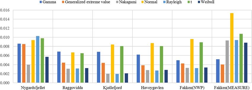
www.nature.com/scientificreports/
energy at a site is to use its annual wind speed distribution. The PDF of wind speed is vital in valuing energy
production for wind power and is an important evaluation index for estimating local wind resource potential.
Related work. Some prior research on wind resources is based on probability distribution methods for spe-
cific regions with varying wind conditions and wind power potential. The two-parameter Weibull distribution
is a widely used statistical distribution in wind engineering9,10; however, the fitting results are not optimal for
some regions, which results in a substantial difference between the estimated annual power generation and the
actual yearly power g eneration5. This suggests that distribution may not be a good representation of some wind
conditions or some sites. Elsewhere, researchers have expressed concerns over the role of case studies for practi-
cal wind engineering purposes. Aries et al. conducted a case study of four sites’ wind speed with eight distribu-
tion models for four sites in Algeria and found that the Generalised extreme value and Gamma Distributions
were the most reliable base on the root mean square error e valuation11. Wang et al. compared parametric and
nonparametric models for wind speed probability distribution by taking four sites in central China as examples
and showed the edge of nonparametric m odels5. Alavi et al. demonstrated that the most suitable probability dis-
tributions for evaluating wind speed were not the same based on five different measurement stations distributed
in the east and south-east of I ran12. Ayodele et al. used the Weibull distribution to estimate the wind resource
in a coastal area of South Africa with complex t errain13. Gualtieri et al. focused on coastal locations in Southern
Italy and used the Weibull distribution extrapolating model to assess wind resource to the turbine hub height14.
Allouhi et al. also used the Weibull distribution to describe the frequencies of actual wind data in six coastal loca-
tions in Morocco based on hourly wind speeds and directions data of 5 years between 2011 and 2 01515. Jiménez
et al. found that atmospheric stability plays a major role in controlling the shape of the wind speed distribution.
The authors showed that the shape wind speed measured from a combination of long-term wind observations
and numerical simulations is strongly modulated by the numerical atmospheric s cales16.
Most studies in this field have focused on PDF modelling for the observed wind speed of wind parks, and
there is a lack of PDF modelling for wind speed forecasted by Numerical Weather Prediction (NWP). This is
unfortunate because NWP calculations generate the vast majority of the world’s wind data. Some studies have
focused on using the Weibull distribution or one of three or four other similar distribution methods. However,
they fail to consider the broader deployment of the PDF approach for wind speed modelling. In practice, more
attention is paid to the wind speed range corresponding to the wind turbine’s rated power. Despite this, few stud-
ies have applied PDF methods to analyse wind speed intervals when wind turbines are producing the maximum
power, and little research has discussed wind speed distribution in the Arctic region.
Objectives. In this research, we comparatively assess seven different probability distributions for wind speed
modelling, some of which are classical, while others have rarely been used to estimate the wind speed distribu-
tion for five wind parks in the Norwegian Arctic coastal region. To improve the understanding of differences in
wind speed data from different resources, we compared wind speed distributions for a wind park with NWP and
observed wind data.
The main contributions of this paper can be summarised as follows.
1. The present study is the first to conduct a PDF modelling analysis of wind speed intervals associated with
wind turbine trunnion rated power, with a particular focus on differences between interval and overall wind
speed modelling.
2. This paper compares wind speed distributions based on wind data from NWP and measurements. Wind
speed distributions provide an intriguing and well-established approach to analyse wind speed resources,
and this paper investigates their use for NWP models in the context of complex coastal terrain.
3. The present study can assist in a more detailed understanding of PDF applications in wind speed modelling,
as seven ideal distributions are used to model wind speed. Moreover, it offers an insight into the potential
for renewable energy utilisation in the Arctic by conducting natural resource modelling in this area, with
clear implications for practice, policy and future project implementation.
The paper is organised as follows: in “Description of wind park and wind speed data”, we describe the wind
data and their sites to provide the context of the study. In “Methodology”, we elaborate on the methodological
aspects of the study, while “Experiment setup and evaluation” outlines the experimental process. “Results and
discussion” presents the results and main implications of the study and reflects on their relevance for research
and practice. The final and concluding section summarises the most important elements of the research.
Description of wind park and wind speed data
In the present study, we focus on five wind parks in the Norwegian Arctic regions. The second and third columns
of Table 1 list their locations and the site ruggedness index (RIX)17. The RIX is an empirical parameter for meas-
uring the complexity of nearby terrain and is typically used in fluid modelling or in numerical weather models
to indicate identify turbulence may interfere with the model results. In our case, this was based on a fraction of
the area within a 2 km radius around the location with a more than 30% degree inclination and was extracted
from a Norwegian mapping of wind resources.
Numerical weather prediction. Scandinavian meteorological institutes use an operational numerical
weather prediction (NWP) forecast known as the Meteorological Ensemble Prediction System (MEPS). The
NWP model is a complex mathematical model of the atmosphere that divides the Earth’s surface into grids18. The
Scientific Reports | (2021) 11:7613 | https://doi.org/10.1038/s41598-021-87299-4 2
Vol:.(1234567890)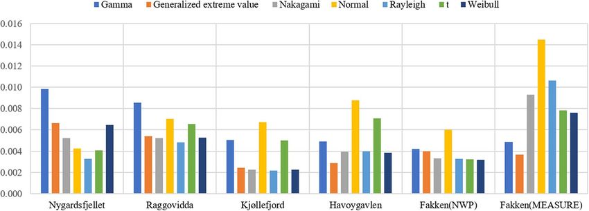
www.nature.com/scientificreports/
Standard
Location deviation Coefficient
Wind park °N/°E RIX Mean (m/s) (m/s) Min (m/s) Max (m/s) of variation Skewness Kurtosis
Nygårdsfjellet 68.504/17.879 0–5 8.096 5.038 0.032 31.481 0.622 0.775 3.815
Raggovidda 70.098/20.081 5–10 9.490 5.101 0.107 32.430 0.538 0.666 3.361
Kjøllefjord 70.769/29.094 0–5 7.900 4.213 0.080 25.508 0.533 0.704 3.453
Havøygavlen 70.922/27.268 10–20 8.335 4.434 0.097 26.926 0.532 0.709 3.359
Fakken
71.012/24.589 5–10 6.948 3.885 0.097 33.686 0.559 1.164 5.960
(NWP)
Fakken
71.012/24.589 5–10 7.687 4.627 0.000 35.100 0.602 1.338 5.660
(MEASURE)
Table 1. The location of wind parks and statistics of their wind speed.
grid’s spatial resolution determines how meteorological processes are simulated with different accuracy levels,
which limits the quality of the forecasts. A study conducted by the Norwegian Meteorological Institute dem-
onstrated that the higher-resolution regional NWP model did not lead to better wind power forecasts for some
Norwegian wind p arks19. Therefore, in the present study, we considered NWP data with a horizontal resolution
of 2.5 km as a relatively coarse resolution in wind predictions.
Data description. NWP wind data from the five wind parks were extracted from Norwegian Meteoro-
logical Institute’s operational MEPS models. The predictions initiated at 00, 06, 12 and 18 UTC and were made
available for operational use about 2 h later. The observed wind data were offered by Troms Kraft AS—the power
company that operates Fakken wind park. In the present study, we combined the forecast data into a single time
series with hourly wind speed data from 0:00 on 1 January 2017 to 23:00 on 31 December 2017. The year is with
wind conditions of northern Norway coastline are not significantly different from the previous 15 years. Table 1
provides a summary of the overall data. The coefficient of variation is defined as the standard deviation divided
by the mean.
Methodology
Wind energy. In wind engineering, the capacity factor (CF) is particularly useful when conducting a fast
evaluation at the early design and planning stages of a wind park. Understanding the probability distribution of
wind speed is essential to calculating the CF of wind parks. The CF is calculated from the average value of wind
energy produced divided by the rated wind power by a wind turbine in a certain period, which may be read from
the following Eqs. (1–3):
Pave
CF = (1)
Pr
∞
Pave = ∫ f (v)P(v)dv (2)
0
Pr vr < v ≤ vo
P(v) = Pr × g(v) vi < v ≤ vr (3)
0 v ≤ vi , v > v0
where f(v) is the PDF of wind speed, which is the main target of this research P(v) reflects the turbine power
curve used to describe the power fluctuations related to wind speed. vi, vr, vo, and Pr represent the cut-in speed,
the rated speed, the cut-off speed, and the rated power, r espectively5,20. The g(v) is a multiplier increasing from
0 to 1 within the interval, that depends on the wind turbine specification. A wind turbine reaches its maximum
power output when the wind speed is in the interval between the rated and cut-off speed. Adequate knowledge
of the wind speed interval corresponding to the wind turbine’s rated power is important for ensuring the efficient
and economical operation of the turbine. Therefore, aside from the wind speed distribution modelling, we also
paid special attention to wind speed in this rated power interval.
Probability distribution. Tables 2 and 3 offer brief mathematical expressions of the seven ideal probability
distributions used in the present study. These distributions are defined as follows.
• Gamma distribution is a two-parameter continuous probability d istribution21.
• Generalised extreme value distribution (GEV) is a continuous probability distribution developed with
extreme value t heory22.
• Nakagami distribution is a generalised two parameters probability distribution model proposed by Nakagami
Minoru23. It has received extensive attention, as it can model a broad range of fading channel conditions and
describe many empirical data s ets24.
Scientific Reports | (2021) 11:7613 | https://doi.org/10.1038/s41598-021-87299-4 3
Vol.:(0123456789)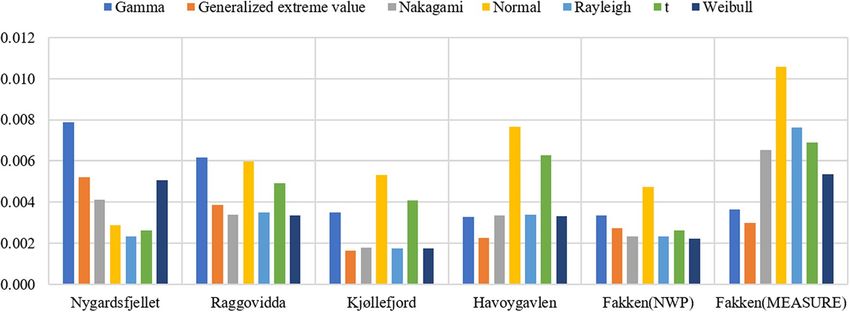
www.nature.com/scientificreports/
Distribution PDF Note CDF
1
x t
f (x; a, b) = ba Ŵ(a) 0 t a−1 e− b dt
where a is a shape parameter
Gamma F(x) = e−t(x)
−1/ξ b is a scale parameter and Ŵ(.) is the Gamma function
t(x) = 1 + ξ x−µ
σ ξ �= 0
e−(x−µ)/σ ξ =0
µ is a location parameter x
GEV f (x; µ, σ , ξ ) = 1
t(x)ξ +1 e−t(x) σ > 0 is a scale parameter F(x; a, b) = 1 a−1 e− bt
σ ba Ŵ(a) 0t dt
ξ is a shape parameter
γ (m, m 2
�x )
m ≥ 1/2 is a shape parameter ≥ 0 is a spread F(x; m, �) = Ŵ(m)
Nakagami 2mm
f (x; m, �) = Ŵ(m)�m x
2m−1 exp −m 2
� x , ∀x ≥ 0 parameter where γ (.) is the Incomplete Gamma function and Ŵ(.)
is the Gamma function
x−µ
2 µ is the mean x−µ
−1
Normal f (x) = √1 e 2 σ σ is the standard division F(x) = � = 1
1 + erf x−µ
√
σ 2
σ 2π
erf (.) is the error function σ 2
Rayleigh f (x; σ ) = x −x 2 /(2σ 2 )
e , x≥0 σ > 0 is a scale parameter F(x; σ ) =
2 2
1 − e−x /(2σ )
σ2
Ŵ ν+1 x Ŵ ν+1
f (x; ν) = 2 √1 1
ν > 0 is the number of degrees of freedom and Ŵ(.) is F(x; ν) = 2 √1
1
dt
t Ŵ ( ν2 ) νπ
x 2
ν+1 Ŵ ( ν2 ) νπ ν+1
1+ ν 2
the Gamma function −∞ 2
1+ tν 2
k−1 k
k
k x
e−(x/ ) x ≥ 0 k > 0 is a shape parameter and > 0 is a scale 1 − e−(x/ ) x ≥ 0
Weibull f (x; , k) = F(x; , k) =
0 x2
2
Weibull Ŵ 1 + k1 2 Ŵ 1 + k2 − Ŵ 1 + k1
Table 3. The mean and variance expressions of distributions.
• Normal distribution, also called Gaussian distribution, is a continuous probability distribution for ideally
describing a real-valued random v ariable25.
• Rayleigh distribution essentially describes the distribution of the mode of a stochastic two-dimensional
vector when the two components of the vector are independent, have the same variance and are normally
distributed with zero means26,27.
• T distribution is commonly used to estimate the mean of a small population that is normally distributed,
where the standard deviation is u nknown28.
• Weibull distribution is the theoretical basis for reliability analysis and life inspections and is widely used for
describing the probability distribution of wind s peed29.
Parametric estimation. Parametric estimation for the PDFs of wind speed refers to the assumption that
a specific probability distribution model can describe the wind speed, where the parameters of the model are
estimated based on available wind speed data. Several parametric estimation methods can be used in wind
engineering, including the moment method, empirical approach, graphical method and maximum likelihood
method30. In a study comparing six methods for estimating Weibull parameters to fit wind data, the maximum
likelihood method was, on the whole, shown to provide more accurate estimations than other methods in tests
with both simulated and observation d ata31. Therefore, we used the maximum likelihood method to identify the
parameters for all seven probability density functions in the present study. The Maximum likelihood estimation
(MLE) method can be explained as follows32: if {X1, X2, …, Xn} is an independent and identically distributed
sample from a population with PDF f (x|θ1 , . . . θk ). The likelihood function is defined by Eq. (4):
Scientific Reports | (2021) 11:7613 | https://doi.org/10.1038/s41598-021-87299-4 4
Vol:.(1234567890)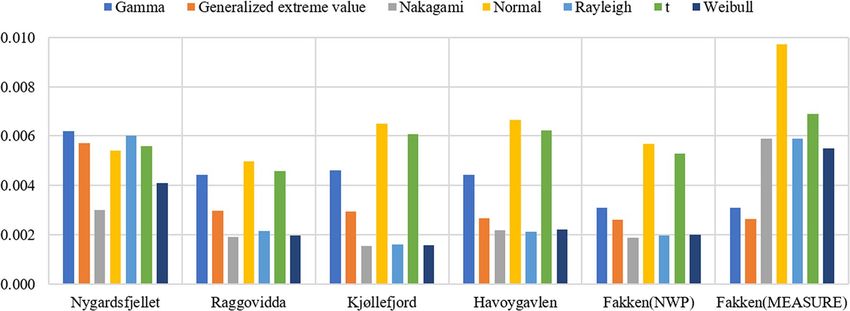
www.nature.com/scientificreports/
n
L(θ|X ) = L(θ1 , . . . θk |x1 · · · xn ) = f (xi |θ1 , . . . θk ) (4)
i=1
If L(θ|X ) is differentiable in θ, then the values of θi that minimize L(θ1 , . . . θk |x1 · · · xn ). are solutions of
possible candidates θi for the MLE are calculated by Eq. (5):
∂
L(θ|X ) = 0, i = 1, 2, . . . k (5)
∂θi
Performance comparison. The Friedman test is used to check for differences in performance across mul-
tiple trials to accurately compare the modelling performance of different probability distributions in different
wind parks33. In particular, column effects are checked after adjusting with possible row effects. The significant
level of the Friedman test was set as 0.01 in the present study.
H0: The column data do not have a significant difference.
Ha: The column data have a significant difference.
The statistic F is shown as in (6):
k
12n
k(k + 1)2
2
F= ri − (6)
k(k + 1) 4
i=1
where k is the number of columns, ri is the mean value of row i. It follows χ(k−1)
2 under H0.
Experiment setup and evaluation
Estimation of PDF. We used 0.5 m/s as the bin size to create histograms of hourly wind speed throughout
the whole year for the wind speed data from the NWP models at the five wind parks and the observed wind
speed of the Fakken wind park. The MLE method was then used to estimate the parameters required to define
each of the theoretical PDFs, as described in “Parametric estimation”. A one-sample Kolmogorov–Smirnov test
(K–S test) was conducted to confirm whether the original wind speed data came from calculated ideal distribu-
tions by comparing the CDF of the original data and fitted ideal distributions.
Since the histogram is discrete, the kernel distribution is typically taken an empirical nonparametric PDF
modelling method based on the original data. It harnesses the kernel functions (typically Gaussian function)
to connect adjacent bins of the histogram to create continuous PDFs of the data. Unlike histograms, the kernel
distribution approximates infinitesimal length sampling, thereby reducing sampling errors between each bin.
Therefore, it can be considered a more real historical distribution of raw data. Graphically, we named this ‘PDF
smoothing’, and it was defined by a kernel function K(·) and a bandwidth d in (7):
n
1
x − xi
fd (x) = K (7)
nd d
i=1
We conducted two separate modelling analyses—overall and interval wind speed PDF fitting—to achieve a
better understanding of the probabilistic characteristic of wind. Based on five wind park features and wind tur-
bine power curve characteristics of our six cases, we choose the wind speed interval related to the rated power,
with the rated speed of 10 m/s and the cut-off speed of 20 m/s, which are typical parameters for commercial
medium-size wind turbines.
Performance evaluation criteria. The K–S test is a nonparametric statistical test based on cumulative
istribution34. A nonpara-
distribution function that tests whether a distribution is different from a type of ideal d
35
metric test is used to test a hypothesis .
H0: {X1, X2, …, Xn} has a given continuous distribution.
Ha : At least one does not come from the given distribution.
The K–S test is constructed from the statistic in Eq. (8):
D = sup|F0 (x) − F(x)| (8)
x
where F0 (x) represents CDF of the given ideal distribution, and F(x) is CDF of {X1, X2, …, X
n}. The test statistic
is compared to critical values from the theoretical distribution of the Brownian bridge (If a Brownian motion,
which is the random motion of particles suspended in a medium, starts at a certain point and returns to the
starting point at the end, the process is called Brownian bridge)36.
To evaluate and compare the different examined performance of PDFs for modelling the wind speed, the
mean absolute error (MAE) and root mean square error (RMSE) were used to calculate the probability density
difference between parametric ideal distributions and the original PDF smoothing with speed unit of 0.01 m/s.
Both are negatively oriented metrics, indicating that the smaller values are related to better performance. The
Scientific Reports | (2021) 11:7613 | https://doi.org/10.1038/s41598-021-87299-4 5
Vol.:(0123456789)www.nature.com/scientificreports/
MAE and RMSE determine the accuracy of a model by calculating averages of the absolute and square difference
between the histogram-based PDF from the NWP and observed data and different theoretical PDF models, as
expressed in Eqs. (9) and (10). The RMSE assigns a higher weight to larger errors due to the square calculation,
which penalises more significant model errors and indicates whether the model has a significant error v ariance37.
Hence, the MAE and RMSE provide a comprehensive representation of a model’s performance
n
i=1 modeling i − smoothing i (9)
MAE =
n
n
2
i=1 modeling i − smoothing i (10)
RMSE =
n
Results and discussion
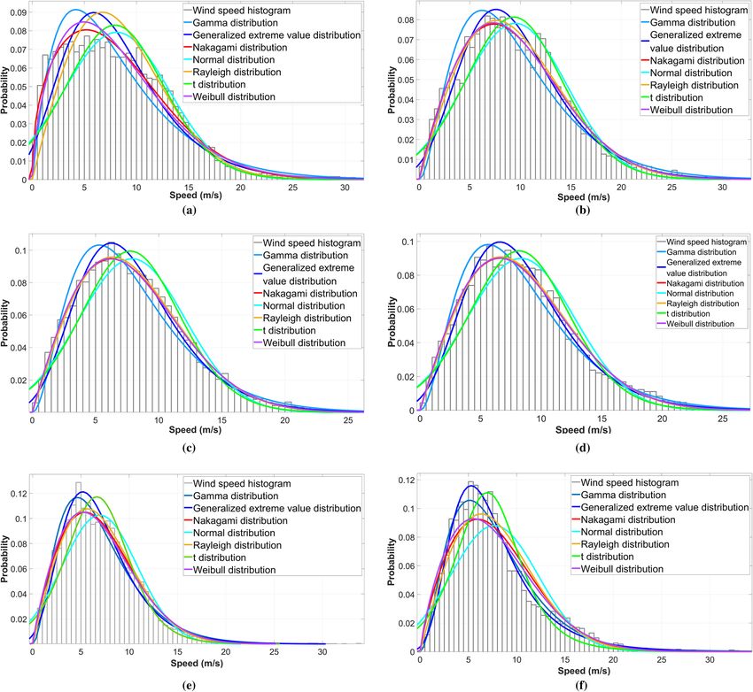
PDF modelling graph. Histograms and PDFs graphs are shown in Fig. 1 to show the estimated ideal PDFs
with the MLE method for different cases. Discontinuous histograms are represented by bar charts (for clarity, we
ignored the kernel distribution curves in these figures), and the fitted probability distribution curves are shown
in different colours. As can be seen, although the wind speed distributions of different wind parks varied, they
had some similarities. It is also clear that different probabilistic models provide differing fits to wind speeds. In
particular, when comparing (e) and (f), the actual wind speed is more centrally concentrated and possesses a
thicker tail. Due to the scarcity of data, this phenomenon could only be considered empirical for the Fakken site.
K–S test. The K–S test is a rigorous statistical test. Passing this test indicates that there is no statistically sig-
nificant difference between the PDFs of original data and ideal distributions. The null hypothesis in the present
study was that wind speed data fit a mentioned ideal distribution; however, they also could not originate from
such an ideal distribution. The significance level was set at 1%, and the results of the K–S test are given in Table 4.
’Pass’ means that the K–S test did not reject the null hypothesis, and ’Fail’ indicates that the K–S test rejected the
null hypothesis.
As is shown, none of the distributions could pass all the K–S tests at the 1% significance level. In addition,
the Gamma, normal and t distributions failed the tests in all cases. Meanwhile, the Nakagami and Weibull
distributions passed the test for three of the NWP wind data sets, while no distributions passed the tests for
Nygårdsfjellet. Regarding the comparison of the PDF modelling between the NWP and observed wind speed
of Fakken, all distributions failed the tests for Fakken (NWP), and only the GEV distribution passed the test
for Fakken (MEASURE). Therefore, the different probabilistic models each have particular strengths that vary
according to wind park and data types.
Overall wind speed PDF modelling. Table 5 shows the calculated parameters by MLE of different PDF
models.
The overall MAE of wind speed PDF fitting for the NWP model from five sites and measurements from Fak-
ken is given in Fig. 2. For the NWP wind speed data, the Nakagami distribution generally had a lower MAE than
the other distributions. One exception to this is Havøygavlen, in which the Rayleigh distribution performed the
best. The normal t distributions had the worst performance in terms of MAE. For the Nakagami distributions
for NWP wind speed from different wind parks, the MAEs of Kjøllefjord and Fakken (which are characterised
by rougher terrain) were lower compared with the other wind parks. For the observed wind speed data fitting of
Fakken, the GEV distribution had the lowest MAE; here, the edge was even more significant than the Nakagami
distribution for Fakken NWP data modelling. In addition, the overall MAE of Fakken measured wind speed
modelling was much larger than for the NWP data of Fakken.
The overall RMSE of the overall wind speed PDF for the NWP model of five sites and measurements of Fakken
wind park is displayed in Fig. 3. In relation to NWP wind speed data, the Nakagami and Rayleigh distributions
showed a low RMSE between the histogram and parameterised PDFs, except for Nygårdsfjellet. The overall
RMSE of the normal and t distributions was relatively high. Kjøllefjord had the lowest RMSE in the Nakagami
and Rayleigh distribution. In terms of the RMSE of wind speed measured data from Fakken, the results were
similar to the overall MAE results.
Friedman tests for the overall MAE and RMSE of wind speed PDF modelling for the NWP data from five sites
were conducted to determine whether there were statistical differences between different probability distribution
modelling approaches (effect of distributions) and whether there were statistical differences in the probabilistic
modelling results for different wind parks (effect of parks). All the p values surpassed the confidence level of 0.01;
therefore, the Friedman test’s null hypothesis was not rejected. The results are shown in Table 6.
Interval wind speed PDF modelling. The MAE of interval wind speed PDF is shown in Fig. 4. The results
showed some differences from their counterparts in the overall modelling. For the NWP wind speed data, the
optimal for Nygårdsfjellet was obtained with the Rayleigh distribution. The Weibull distribution had a slight
advantage over the Nakagami and Rayleigh distributions, while the normal distribution showed the worst MAE
performance on the whole. The MAE of the Weibull distributions for Kjøllefjord were the smallest out of the five
wind parks. Regarding the distributions of measured wind speed of Fakken, the overall MAE was much larger
than for the Fakken NWP data; further, the GEV produced the lowest MAE.
Scientific Reports | (2021) 11:7613 | https://doi.org/10.1038/s41598-021-87299-4 6
Vol:.(1234567890)www.nature.com/scientificreports/
Figure 1. The estimated PDFs curve graphs for NWP model data of five sites and measurements from
Fakken wind park (NWP: (a) Nygårdsfjellet, (b) Raggovidda, (c) Kjøllefjord, (d) Havøygavlen, (e) Fakken,
Measurements: (f) Fakken).
Wind park Gamma GEV Nakagami Normal Rayleigh t Weibull
Nygårdsfjellet Fail Fail Fail Fail Fail Fail Fail
Raggovidda Fail Fail Pass Fail Fail Fail Pass
Kjøllefjord Fail Fail Pass Fail Pass Fail Pass
Havøygavlen Fail Pass Pass Fail Pass Fail Pass
Fakken (NWP) Fail Fail Fail Fail Fail Fail Fail
Fakken (MEASURE) Fail Pass Fail Fail Fail Fail Fail
Table 4. The result of the K–S test.
Scientific Reports | (2021) 11:7613 | https://doi.org/10.1038/s41598-021-87299-4 7
Vol.:(0123456789)www.nature.com/scientificreports/
Gamma GEV Nakagami Normal Rayleigh t Weibull
Nygardsfjellet 2.07; 3.91 5.80; 4.10; − 0.02 0.72; 90.93 8.10; 5.04 6.74 17.87 1.62; 9.02
Raggovidda 2.90; 3.27 7.26; 4.10; − 0.07 0.94; 116.08 9.50; 5.10 7.62 20.66 1.93; 10.69
Kjøllefjord 3.04; 2.60 6.04; 3.10; − 0.05 0.97; 80.15 8.10; 5.04 6.33 16.67 1.96; 8.91
Havoygavlen 3.07; 2.71 6.37; 3.10; − 0.05 0.98; 89.14 8.34; 4.43 6.68 16.84 1.96; 9.40
Fakken (NWP) 2.99; 2.32 5.18; 3.10; 0.00 0.94; 63.37 6.95; 3.89 5.63 7.48 1.87; 7.83
Fakken (MEASURE) 3.01; 2.56 5.54; 3.10; 0.08 0.90; 79.62 7.69; 4.53 6.31 4.26 1.80; 8.68
Table 5. The parameters of fitted PDFs. The parameters are shown with the form in Table 2 in order
corresponding to each PDF.
Figure 2. The overall MAE of wind speed PDFs for NWP data from five sites and measurements from Fakken.
Figure 3. The overall RMSE of wind speed PDFs for NWP data from five sites and measurements from Fakken.
Effect of distributions Effect of parks
MAE 0.0011 0.0525
RMSE 0.0014 0.0029
Table 6. The p values of the Friedman test for overall wind speed modelling.
The RMSE of the interval wind speed PDF is shown in Fig. 5. The results were similar to the MAE evaluation
of interval modelling. For the NWP wind speed data, the Rayleigh distribution was superior to other distribu-
tions for Nygårdsfjellet. The Nakagami, Rayleigh and Weibull distributions had almost the same RMSEs for the
remaining four wind parks, while for the RMSE of the observed data from Fakken, the GEV distribution still won.
Similarly, differences in interval wind speed from NWP probabilistic modelling between wind parks were
tested, and the results are given in Table 7. All p values exceeded the confidence level of 0.01, which suggests
Scientific Reports | (2021) 11:7613 | https://doi.org/10.1038/s41598-021-87299-4 8
Vol:.(1234567890)www.nature.com/scientificreports/
Figure 4. The MAE of interval wind speed PDFs for NWP data from five sites and measurements from Fakken.
Figure 5. The RMSE of interval wind speed PDFs for NWP data from five sites and measurements from
Fakken.
Effect of distributions Effect of parks
MAE 0.0717 0.05
RMSE 0.0156 0.0134
Table 7. The p values of the Friedman test for interval wind speed modelling.
that there are statistical differences between different probability distribution modelling methods and in the
probabilistic modelling of different wind parks.
Discussion. In summary, the Nakagami distribution is recommended as the preferred model for the PDF of
NWP wind speed data, as it showed excellent and consistent performance. The Nakagami and Weibull distribu-
tions could generally capture essential characteristics of the historical distributions of wind speed for both NWP
model data by K–S tests. The GEV distribution could describe the statistics of the observed wind data in the
examples we used. Moreover, PDF modelling for the NWP wind speed was more accurate compared with actual
measurements of wind speed.
In terms of evaluating the NWP wind speed, for the overall wind speed PDF modelling performance, the
Nakagami and Weibull distributions showed a good fit for all five wind parks’ overall PDFs of NWP wind speed
data. In comparison, the Rayleigh distribution provided a favourable overall fit for all except Nygårdsfjellet. The
Nakagami and Rayleigh distributions also performed excellently for the wind speed interval modelling. Generally,
we made a more precise PDF fitting for NWP wind speed data from Kjøllefjord than for other wind parks both in
overall and interval wind speed modelling. This was unexpected, as Kjøllefjord has the highest RIX (10–20) of all
of them. In addition, Havøygavlen and Fakken, with RIXs (5–10), were also fitted better than Nygårdsfjellet and
Raggovidda with RIXs (0–5). Further research is needed because it is generally thought that the more complex
the terrain is, the more difficult it is to use NWP to forecast the wind speed38.
For the actual observed wind data from Fakken, the GEV distribution was superior to all other distributions
both in overall and interval wind speed modelling and should be used to assess wind speed in this area. The
Scientific Reports | (2021) 11:7613 | https://doi.org/10.1038/s41598-021-87299-4 9
Vol.:(0123456789)www.nature.com/scientificreports/
differences between NWP wind data and real measurements of Fakken can be summarised as follows. First,
referring to Table 2, the observed speed had a higher mean value, standard deviation, coefficient of variation
and skewness, though lower kurtosis meant that the measurements varied more from the normal distribution
and had a lighter distribution tail than the NWP data. Second, the best distributions were the Nakagami and
Generalised extreme value distribution, respectively. The Weibull distribution, which is typically used for wind
speed modelling, was inferior to these two methods in our cases.
Conclusions
The statistical characteristics of wind speed are essential for the practical assessment of wind energy potential and
the sustainable design of wind parks. In the present study, we concentrated on probabilistic modelling of NWP
wind speed for five wind parks in the Norwegian Arctic region and one observed wind speed for one of them.
Our results are based on 1 year of data, and a longer period is needed to conduct a wind resource assessment of a
potential wind park site. Using longer time series would provide a better estimate of the wind speed distribution
for NWP and measurements and a better understanding of rare extreme high wind events. The results of the
present study indicated that, for wind resource assessments in complex terrain, the Nakagami and Generalised
extreme value distributions are recommended as the preferred models for the PDF of NWP and observed wind
speed, respectively, as they showed excellent and consistent performance. In addition, the probabilistic models
that reasonably describe interval wind speed differ from those of overall wind speed due to the nature of the wind:
the former corresponds more to the right-side properties of the probability distribution functions.
Based on the results of this study, the following policy recommendations are provided.
1. Different probabilistic modelling approaches should be considered when conducting wind resource potential
assessments to achieve more accurate estimations.
2. The wind speeds of neighbouring regional wind parks are characterised by similarities and synergies partly
due to the probabilistic models that accurately describe them are identical. But in wind engineering real-
ity, Topography, meteorology, turbine selection and layout etc. all affect the power generation of a wind
park. Therefore, the possibility of simultaneous intermittency of these wind parks must be considered when
exploiting wind power in the area. Reasonable compensations for other energy sources are required.
3. Compared with observed wind speeds, numerical predicted speeds can be better described by probabilistic
models; therefore, when using numerical meteorology to assess wind resources, more consideration should
be given to extreme wind events. Some allowance may be made for errors in wind energy project develop-
ment.
Data availability
The NWP data is public available from The Norwegian Meteorological Institute. The measured wind data from
Fakken wind park is the property of the power company Troms Kraft AS.
Received: 5 February 2021; Accepted: 26 March 2021
References
1. Zeng, P., Sun, X. & Farnham, D. J. Skillful statistical models to predict seasonal wind speed and solar radiation in a Yangtze River
estuary case study. Sci. Rep. 10, 1–11 (2020).
2. Nazir, M. S., Ali, N., Bilal, M. & Iqbal, H. M. Potential environmental impacts of wind energy development: A global perspective.
Curr. Opin. Environ. Sci. Health 13, 85–90 (2020).
3. Association, E. W. E. Wind Energy-the Facts: A Guide to the Technology, Economics and Future of Wind Power (Routledge, 2012).
4. Yuan, J. Wind energy in China: Estimating the potential. Nat. Energy 1, 1–2 (2016).
5. Wang, J., Hu, J. & Ma, K. Wind speed probability distribution estimation and wind energy assessment. Renew. Sustain. Energy Rev.
60, 881–899 (2016).
6. Jain, P. Wind Energy Engineering (McGraw-Hill Education, 2016).
7. Bilal, M., Birkelund, Y., Homola, M. & Virk, M. S. Wind over complex terrain–Microscale modelling with two types of mesoscale
winds at Nygårdsfjell. Renew. Energy 99, 647–653 (2016).
8. Safari, B. & Gasore, J. A statistical investigation of wind characteristics and wind energy potential based on the Weibull and Rayleigh
models in Rwanda. Renew. Energy 35, 2874–2880 (2010).
9. Akdağ, S., Bagiorgas, H. & Mihalakakou, G. Use of two-component Weibull mixtures in the analysis of wind speed in the Eastern
Mediterranean. Appl. Energy 87, 2566–2573 (2010).
10. Ozay, C. & Celiktas, M. S. Statistical analysis of wind speed using two-parameter Weibull distribution in Alaçatı region. Energy
Convers. Manage. 121, 49–54 (2016).
11. Aries, N., Boudia, S. M. & Ounis, H. Deep assessment of wind speed distribution models: A case study of four sites in Algeria.
Energy Convers. Manage. 155, 78–90 (2018).
12. Alavi, O., Mohammadi, K. & Mostafaeipour, A. Evaluating the suitability of wind speed probability distribution models: A case
of study of east and southeast parts of Iran. Energy Convers. Manage. 119, 101–108 (2016).
13. Ayodele, T., Jimoh, A., Munda, J. & Agee, J. Wind distribution and capacity factor estimation for wind turbines in the coastal region
of South Africa. Energy Convers. Manage. 64, 614–625 (2012).
14. Gualtieri, G. & Secci, S. Extrapolating wind speed time series vs. Weibull distribution to assess wind resource to the turbine hub
height: A case study on coastal location in Southern Italy. Renew. Energy 62, 164–176 (2014).
15. Allouhi, A. et al. Evaluation of wind energy potential in Morocco’s coastal regions. Renew. Sustain. Energy Rev. 72, 311–324 (2017).
16. Jiménez, P. A., Dudhia, J. & Navarro, J. On the surface wind speed probability density function over complex terrain. Geophys. Res.
Lett. 38, 22 (2011).
17. Birkelund, Y., Alessandrini, S., Byrkjedal, Ø. & Monache, L. D. Wind power predictions in complex terrain using analog ensembles.
J. Phys.: Conf. Ser 1102, 012008 (2018).
Scientific Reports | (2021) 11:7613 | https://doi.org/10.1038/s41598-021-87299-4 10
Vol:.(1234567890)www.nature.com/scientificreports/
18. Collins, S. N. et al. Grids in numerical weather and climate models. Clim. Change Regional/Local Responses. https://doi.org/10.
5772/55922 (2013).
19. Bremnes, J. B. & Giebel, G. Do regional weather models contribute to better wind power forecasts?. The Norwegian Meteorologi-
calInstitute (2017).
20. Masseran, N., Razali, A. & Ibrahim, K. An analysis of wind power density derived from several wind speed density functions: The
regional assessment on wind power in Malaysia. Renew. Sustain. Energy Rev. 16, 6476–6487 (2012).
21. Burgin, T. The gamma distribution and inventory control. J. Oper. Res. Society 26, 507–525 (1975).
22. Hosking, J. R. M., Wallis, J. R. & Wood, E. F. Estimation of the generalized extreme-value distribution by the method of probability-
weighted moments. Technometrics 27, 251–261 (1985).
23. Nakagami, M. Statistical Methods in Radio Wave Propagation 3–36 (Elsevier, 1960).
24. Rubio, L., Reig, J. & Cardona, N. Evaluation of Nakagami fading behaviour based on measurements in urban scenarios. AEU-Int.
J. Electron. Commun. 61, 135–138 (2007).
25. Lyon, A. Why are normal distributions normal?. Br. J. Philos. Sci. 65, 621–649 (2014).
26. Balakrishnan, N. Approximate MLE of the scale parameter of the Rayleigh distribution with censoring. IEEE Trans. Reliab. 38,
355–357 (1989).
27. Papoulis, A. & Pillai, S. U. Probability, Random Variables, and Stochastic Processes (Tata McGraw-Hill Education, 2002).
28. Rigby, R. A. & Stasinopoulos, D. M. Generalized additive models for location, scale and shape. J. Roy. Stat. Soc.: Ser. C (Appl. Stat.)
54, 507–554 (2005).
29. Rinne, H. The Weibull Distribution: A Handbook (CRC Press, 2008).
30. Saleh, H., Aly, A.A.E.-A. & Abdel-Hady, S. Assessment of different methods used to estimate Weibull distribution parameters for
wind speed in Zafarana wind farm, Suez Gulf, Egypt. Energy 44, 710–719 (2012).
31. Chang, T. P. Performance comparison of six numerical methods in estimating Weibull parameters for wind energy application.
Appl. Energy 88, 272–282 (2011).
32. Myung, I. J. Tutorial on maximum likelihood estimation. J. Math. Psychol. 47, 90–100 (2003).
33. Gibbons, J. D. & Chakraborti, S. Nonparametric Statistical Inference: Revised and Expanded (CRC Press, 2014).
34. Justel, A., Peña, D. & Zamar, R. A multivariate Kolmogorov–Smirnov test of goodness of fit. Statist. Probab. Lett. 35, 251–259
(1997).
35. Hollander, M., Wolfe, D. A. & Chicken, E. Nonparametric Statistical Methods Vol. 751 (Wiley, 2013).
36. Marsaglia, G., Tsang, W. W. & Wang, J. Evaluating Kolmogorov’s distribution. J. Stat. Softw. 8, 1–4 (2003).
37. Li, L. et al. A half-Gaussian fitting method for estimating fractional vegetation cover of corn crops using unmanned aerial vehicle
images. Agric. For. Meteorol. 262, 379–390 (2018).
38. Cassola, F. & Burlando, M. Wind speed and wind energy forecast through Kalman filtering of Numerical Weather Prediction
model output. Appl. Energy 99, 154–166 (2012).
Acknowledgements
The open access publication charges for this article have been funded by a Grant from the publication fund of
UiT The Arctic University of Norway.
Author contributions
H.C. is responsible for developing methods, conducting experiments, drawing charts, analyzing results, and
writing the original draft. Y.B. is responsible for data curation, methodology improvements, and supervisions.
S.N.A., R.S.-D., and F.Y. help in statistical methods results analysis and writing review and editing.
Competing interests
The authors declare no competing interests.
Additional information
Correspondence and requests for materials should be addressed to H.C.
Reprints and permissions information is available at www.nature.com/reprints.
Publisher’s note Springer Nature remains neutral with regard to jurisdictional claims in published maps and
institutional affiliations.
Open Access This article is licensed under a Creative Commons Attribution 4.0 International
License, which permits use, sharing, adaptation, distribution and reproduction in any medium or
format, as long as you give appropriate credit to the original author(s) and the source, provide a link to the
Creative Commons licence, and indicate if changes were made. The images or other third party material in this
article are included in the article’s Creative Commons licence, unless indicated otherwise in a credit line to the
material. If material is not included in the article’s Creative Commons licence and your intended use is not
permitted by statutory regulation or exceeds the permitted use, you will need to obtain permission directly from
the copyright holder. To view a copy of this licence, visit http://creativecommons.org/licenses/by/4.0/.
© The Author(s) 2021
Scientific Reports | (2021) 11:7613 | https://doi.org/10.1038/s41598-021-87299-4 11
Vol.:(0123456789)You can also read