A Decision Support System for Dynamic Job-Shop Scheduling Using Real-Time Data with Simulation - MDPI
←
→
Page content transcription
If your browser does not render page correctly, please read the page content below
mathematics
Article
A Decision Support System for Dynamic Job-Shop
Scheduling Using Real-Time Data with Simulation
Ahmet Kursad Turker * , Adnan Aktepe , Ali Firat Inal , Olcay Ozge Ersoz ,
Gulesin Sena Das and Burak Birgoren
 Department of Industrial Engineering, Kirikkkale University, 71451 Campus, Turkey; aaktepe@kku.edu.tr (A.A.);
 afinal@kku.edu.tr (A.F.I.); ooersoz@hotmail.com (O.O.E.); senadas@kku.edu.tr (G.S.D.);
 birgoren@kku.edu.tr (B.B.)
 * Correspondence: kturker@kku.edu.tr

 Received: 26 February 2019; Accepted: 14 March 2019; Published: 19 March 2019

 Abstract: The wide usage of information technologies in production has led to the Fourth Industrial
 Revolution, which has enabled real data collection from production tools that are capable of
 communicating with each other through the Internet of Things (IoT). Real time data improves
 production control especially in dynamic production environments. This study proposes a decision
 support system (DSS) designed to increase the performance of dispatching rules in dynamic
 scheduling using real time data, hence an increase in the overall performance of the job-shop.
 The DSS can work with all dispatching rules. To analyze its effects, it is run with popular dispatching
 rules selected from the literature on a simulation model created in Arena® . When the number of jobs
 waiting in the queue of any workstation in the job-shop falls to a critical value, the DSS can change
 the order of schedules in its preceding workstations to feed the workstation as soon as possible.
 For this purpose, it first determines the jobs in the preceding workstations to be sent to the current
 workstation, then finds the job with the highest priority number according to the active dispatching
 rule, and lastly puts this job in the first position in its queue. The DSS is tested under low, normal,
 and high demand rate scenarios with respect to six performance criteria. It is observed that the DSS
 improves the system performance by increasing workstation utilization and decreasing both the
 number of tardy jobs and the amount of waiting time regardless of the employed dispatching rule.

 Keywords: industry 4.0; dynamic job-shop scheduling; simulation; decision support systems; internet
 of things

1. Introduction
      Production is the transformation of natural resources to value-added products or services to meet
consumer needs. In order to manage the production well, it is necessary to meet the consumer demands
in terms of price, time, quantity, and quality, while decreasing the inventory levels and increasing the
stock cycle speed/service level. At this point, questions such as which product, how many, which
features, where, and by whom, should be answered to minimize production costs or maximize profits
of an organization.
      In a job-shop production environment, production is mostly carried out according to the customer
order, the due date of which is usually set by the customer. Since the variety of products is high
and the order size is low, production flows (routes) usual change from product to product among
universal machines in the workshop. Therefore, the coordination of production resources in a job-shop
production environment is often difficult. This challenge necessitates the use of advanced production
planning and control systems in job-shop environments.

Mathematics 2019, 7, 278; doi:10.3390/math7030278                          www.mdpi.com/journal/mathematics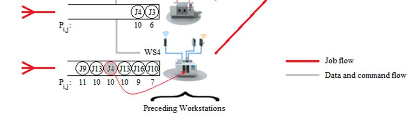
Mathematics 2019, 7, 278 2 of 19
Scheduling is the planning of the activities in the job-shop at the operational level (day, hour,
minute, etc.). When scheduling production, various performance criteria should be considered, such as
(i) timely delivery (minimization of delays), (ii) reduced time spent in the system (minimization of
waitin), and (iii) maximization of machine utilization rates [1].
Mathematics 2019, 7, x FOR PEER REVIEW 2 of 20
In a job-shop, scheduling of jobs is usually performed with static dispatching rules.
This scheduling approach
as (i) timely delivery is ineffective
(minimization because
of delays), it doestime
(ii) reduced not spent
consider
in the dynamic factors likeof new
system (minimization
arriving orders
waitin), and and
(iii)probabilistic
maximizationorofstochastic real-life problems
machine utilization rates [1]. such as job postponement or machine
failures [2]. In Moreover,
a job-shop,research
scheduling showsof jobs
thatisclassical
usually scheduling
performed with fails tostatic
meetdispatching
the needsrules. This
of production
scheduling approach is ineffective because it does not consider
environments in practice [3,4]. Thus, advanced scheduling tools are needed to model this dynamic dynamic factors like new arriving
orders environment.
production and probabilistic or stochastic real-life problems such as job postponement or machine failures
[2]. Moreover, research shows that classical scheduling fails to meet the needs of production
One of the tools to deal with such a dynamic production environment is simulation. Simulation
environments in practice [3,4]. Thus, advanced scheduling tools are needed to model this dynamic
allows modeling and analysis of real-life processes and systems in a computer environment in shorter
production environment.
times withOne lower costs
of the [5–7].
tools to deal with such a dynamic production environment is simulation. Simulation
This study proposes
allows modeling and analysis a decision support
of real-life system
processes and (DSS)
systemsdesigned to increase
in a computer the performance
environment in shorter of
dispatching rules in dynamic
times with lower costs [5–7]. scheduling using real-time data, hence to increase the overall performance
of the job-shop.
This study To proposes
analyze aitsdecision
effects,support
it is run with(DSS)
system popular
designeddispatching
to increase rules selected from
the performance of the
dispatching
literature rules in dynamic
on a simulation model created scheduling
in Arenausing ® . real-time
When thedata, numberhenceofto jobsincrease
waiting theinoverall
the queue
of anyperformance
workstation ofinthethe
job-shop.
job-shop To falls
analyze
to aitscritical
effects,value,
it is run with
the DSS popular dispatching
can change the orderrulesof selected
schedules
from the literature on a simulation model created in Arena ®. When the number of jobs waiting in the
in its preceding workstations to feed the workstation as soon as possible. For this purpose, it first
queue of any workstation in the job-shop falls to a critical value, the DSS can change the order of
determines the jobs in the preceding workstations to be sent to the current workstation, then finds the
schedules in its preceding workstations to feed the workstation as soon as possible. For this purpose,
job with the highest priority number according to the active dispatching rule, and lastly puts this job
it first determines the jobs in the preceding workstations to be sent to the current workstation, then
at thefinds
first position
the job within its
thequeue.
highest priority number according to the active dispatching rule, and lastly
The
puts this job at the firstthe
data needed for DSS includes
position real-time machine and product status including operating
in its queue.
conditions, Theworkstation
data needed queue for the DSS status, workload,
includes real-time etc. The data
machine is collected
and product status from production
including operatingtools
that are capableworkstation
conditions, of communicating queue status, with each other
workload, etc. via
The the
dataInternet
is collected of from
Things (IoT). The
production toolsIoT
thatis the
networkare capable
of devicesof communicating
such as vehicles withand
eachhome
other appliances
via the Internet thatofcontain
Things (IoT). The IoT software,
electronics, is the network sensors,
of devices
actuators, such as vehicles
and connectivity thatand homethese
allows appliances
thingsthat to contain
connect, electronics,
interact, andsoftware, sensors,
exchange actuators,
data. It involves
and connectivity that allows these things to connect, interact,
technologies such as Wi-Fi, Bluetooth, and Radio Frequency Identification (RFID). The functioning and exchange data. It involves of a
technologies such as Wi-Fi, Bluetooth, and Radio Frequency Identification (RFID). The functioning
representative job-shop equipped with the IoT technologies is shown in Figure 1. In manufacturing
of a representative job-shop equipped with the IoT technologies is shown in Figure 1. In
shop floors, use of the IoT has turned machines into smart manufacturing objects that can communicate
manufacturing shop floors, use of the IoT has turned machines into smart manufacturing objects that
with each other,
can communicate enablingwithaccess to vast
each other, amounts
enabling of real
access data
to vast [8]. In of
amounts manufacturing, IoT could generate
real data [8]. In manufacturing,
so muchIoT business value so
could generate thatmuchit is business
believedvalueto lead to itthe
that is Fourth
believedIndustrial
to lead toRevolution, which is also
the Fourth Industrial
referred to as Industry
Revolution, which is 4.0.
also referred to as Industry 4.0.
Figure 1.1.Functioning
Figure Functioning of the system.
of the system.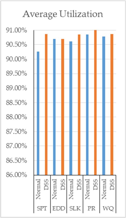
Mathematics 2019, 7, 278                                                                         3 of 19

     This system can be integrated into an Enterprise Resource Planning (ERP) information system to
make scheduling more effective. We believe that improving the efficiency of production management
activities with such approaches could lead to an increase in the demand for Industry 4.0 practices.
     Before introducing the functioning of the proposed system in Section 4, a literature review and
discussion on dispatching rules are presented in Sections 2 and 3, respectively. Later in Section 4,
both the designed system and the developed simulation model are discussed. Finally, conclusions and
future work are supplied in Section 5.

2. Related Work
      In this section, we presented approaches and methods used to determine dispatching rules in
different production environments.
      Marinho et al. [9] developed a decision support system for a dynamic production scheduling
system. They stated that these systems are suitable for small and medium enterprises. In this
study, the manufacturing orders are scheduled dynamically. The scheduling was carried out with
an earliest/latest finish, minimum/maximum slack, smallest free intervals, and minimum delay
heuristics. Deadlines of manufacturing orders and resources occupation were considered in the study.
In addition, an interface was developed in the study for helping managers make faster decisions.
      Aydin and Oztemel [10] developed an approach for the solution of the dynamic job-shop type
scheduling problem by using the agent and the simulated environment. The intelligent agent
determines the most appropriate rule in the real time production environment, whereas scheduling is
carried out using the rule chosen by the simulation technique. The intelligent agent used in the model
is trained with a learning algorithm developed in the study. The results obtained with the developed
smart agent are better than shortest processing time (SPT), cost over time (COVERT), and critical ratio
(CR) rules.
      Li et al. [11], studied on a real time production improvement through bottleneck control.
They stated that a dynamic bottleneck control system is developed in order to efficiently use the
finite manufacturing resources. Their objective was to achieve a continuous production improvement.
The method they developed is applied in an automotive assembly line. As a result, they reduced the
downtime of the bottleneck machine.
      Heilala et al. [12] developed a simulation-based decision support system as an operative
simulation model that enables to handle unforeseen events such as downtime and changes in
operations. In their study, they stated that a simulation-based decision support system could be
used to help achieve more efficient manufacturing. They discussed that data integration, automated
simulation, and the visualization of results in this field.
      Mahdavi and Shirazi [13] presented a review of intelligent decision support systems in production
planning of flexible manufacturing systems. In their study, they developed real time control of the
shop floor. They presented performance criteria for effective and efficient control of the production.
They determined the sequence of the jobs in the system using the developed rules.
      Sharma and Jain [14] examined the dynamic job-shop type scheduling problem in the stochastic
environments by adding the time-dependent preparation times constraint. In the study, makespan,
average flow time, maximum flow time, average tardiness, maximum tardiness, number of tardy
jobs, total setup time, and average setup time were calculated by the developed algorithm. The
JMEDD rule developed in the study gave the best value among all rules. In another study, Sharma and
Jain [15] developed four new rules for the same problem that was considered by them. These rules are:
(1) TDDSSPT: Shortest (time to due date + setup time + processing time); (2) JTDDSSPT: Same setup
time and shortest (time to due date + setup time + processing time); (3) JSLACK: Same setup time and
shortest slack time; and (4) JSLACKW: Same setup time and the shortest slack time per unit job.
      Different from other works, Zhong et al. [16] used data that is obtained from a production
environment using the Radio Frequency Identification (RFID) system. This system collected data and
analyzed these data with data mining to determine standard processing times and dispatching rules.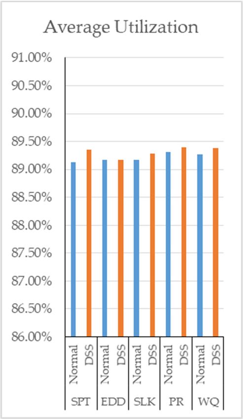
Mathematics 2019, 7, 278                                                                             4 of 19

Next, decision trees were used to find that the use of concurrent data improves the determination of
dispatching rules.
      Kulkarni and Venkatesvaran [17] developed the simulation-based optimization algorithm (SbO)
for job-shop type scheduling problems. They developed a hybrid algorithm to solve the problem.
The developed algorithm has been tested in deterministic and stochastic environments. Obtained
results were better than classical mixed integer programming model.
      Zhong et al. [8] carried out a Big Data Analytics for RFID logistics data by defining different
behaviors of smart manufacturing objects. They developed physical internet-enabled intelligent
shop floor. The task weight was considered in the logistics decision-making. According to results
of the application, the highest residence time occurs in a buffer with the value of 40.57% of the total
delivery time.
      Phanden and Jain [18] developed a genetic algorithm approach that is based on a simulation
model. In their study, the model selects a job that becomes a candidate to change the available process
plans. The objective of the model is to minimize mean tardiness. Three case studies were conducted in
their study. They found that changing the current plan according to algorithm results helped to reduce
mean tardiness.
      Kuck et al. [19] proposed a data-driven simulation-based optimization algorithm for the control
of dynamic production systems. In the present study, it was emphasized that flexibility in production
is very important. They have developed an approach for the re-scheduling of production according to
the new situations considering factors that may cause confusion, such as the simultaneous arrival of a
large amount of orders.
      Ersoz et al. [20] tried to reduce the difference between practice and scheduling theory.
They adapted the real-time information generated by the process control and control systems, to
their planning activities. In the offered system, the dynamic structure of the production environment is
immediately perceived and the schedule is updated according to the new conditions. The traceability of
the parts increased in the factory. In addition, unnecessary waiting or downtimes have been minimized.
      Zhang et al. [21] studied real time job-shop scheduling. In their study, they offered two algorithms:
the simulation-based value iteration and simulation based Q learning, which were developed to solve
the scheduling problem from the perspective of a Markov decision process (MDP). They also used an
intelligent system to estimate value function. The MDP rule is compared with SPT, longest processing
time (LPT), first-in-first-out (FIFO), and CR. It is observed that MDP performed better than others.
      Bierwirth and Kuhpfahl [22] proposed a new approach by synthesizing the GRASP algorithm
with local search methods that minimized the total weighted tardiness in job-shop type scheduling.
The model based on critical tree building produced better results in terms of total processing time
criterion compared to the conventional GRASP algorithm.
      Xiong et al. [23] proposed a simulation-based model for determining dispatching rules in a
dynamic scheduling problem where job release times and extended technical priority constraints are
included. The proposed algorithm reduced the total tardiness and the number of tardy jobs.
      Zhang et al. [24] reviewed the literature on job-shop scheduling problems and discussed new
perspectives under Industry 4.0. They reviewed more than 120 papers. They stated that under
Industry 4.0, the scheduling problems are dealt with new methods and approaches. According to their
findings, scheduling research needs to shift its focus to smart distributed scheduling modeling and
optimization. According their evaluation, this can be achieved with two approaches: (1) combining
traditional methods and proposing a new method and (2) proposing new algorithms for smart
distributed scheduling.
      Rossit et al. [25] described the concept of intelligent production that emerged with Industry 4.0
in their work. They have dealt with the issue of smart scheduling, which they believe to have an
important place in today’s production understanding. They have developed the concept of tolerant
scheduling in a dynamic environment in order to prevent the need for re-scheduling in production.
Similarly, Tao et al. [26] stated that one of the important studies conducted in the literature in the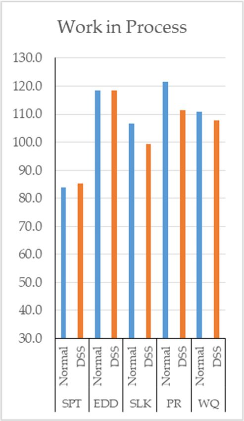
Mathematics 2019, 7, 278                                                                             5 of 19

scope of Industry 4.0 is dynamic scheduling. They examined the recent innovations in production
systems and the smart manufacturing approaches, as well as models that came up with Industry 4.0.
In the study, the analysis of the data life cycle in production and the use of large data in production are
explained. Conceptual models on the use of large data in production is developed and the use of large
data for different sectors is explained with examples.
      Jiang et al. [27] studied an energy-efficient job-shop scheduling problem. Their aim was to
minimize the sum of the energy consumption cost and the completion-time cost. However, the handled
problem was considered NP-Hard. Thus, they developed an improved whale optimization algorithm
for solving this problem. They used dispatching rules, nonlinear convergence factors, and mutation
operation for the improvement of whale optimization algorithm. To show the effectiveness of the
algorithm, they performed simulations. According to results of simulations carried out, the algorithm
provided advantages in terms of efficiency.
      Ortiz et al. [28] analyzed a flexible job-shop problem and proposed a new model for the solution.
They formulated a real-world production-scheduling problem and also provided an efficient tool to
solve it. They developed a new algorithm that minimizes average tardiness and found better solutions
than the existing dispatching rules.
      Ding and Jiang [29] discussed the effect of the IoT technology in a manufacturing environment.
They state that, with IoT, production data increased but that these data are sometimes discrete,
uncorrelated, and hard-to-use. Therefore, they developed a method to use invaluable data.
They provided an RFID-based production data analysis method for production control in IoT-enabled
smart job-shops. In addition, a big data approach was developed to excavate hidden information and
knowledge from the historical production data.
      Leusin et al. [30] developed a multi agent system in a cyber-physical system to solve the dynamic
job-shop scheduling problem. The proposed solution had self-configuring features in the production
line. This was achieved with the use of agents and IoT. Real time data were used for efficient decision
making in the job-shop. The model was tested with a real case study. Under different scenarios,
they gained results that are more efficient than standard dispatching rules. In addition, the advantages
of using dynamic data and IoT in industrial applications are discussed.
      Zhang et al. [31] emphasized the importance of learn concepts in operational management,
especially the importance of the lean approach in Industry 4.0. In this study, process control theory
was used for lean methods. Thus, they proposed Lean-Oriented Optimum-State Control Theory
(L-OSCT) in the study. L-OSCT provides dynamic process control in industrial networking systems.
The application was carried out in a large-size paint making company to show the effectiveness of
the approach.
      After examining the relevant literature, it was observed that several models were developed to
determine dispatching rules in dynamic job-shop type scheduling. As a contribution, we developed a
decision support system for dynamic environments that could work with different dispatching rules.
Our aim was to increase the efficiency of the production management and job-shop.

3. Dispatching Rules in Scheduling
     Scheduling aims to assign jobs to workstations according to a dispatching rule was done to
determine order of processing. These rules are procedures designed to provide good solutions to
complex problems in a real-time production environment [4]. Many researchers have proposed various
dispatching rules to optimize some performance criteria in a production environment. Since the list
of orders to process is updated continuously, the actual problem is dynamic and complex; however,
many classical rules do not take this dynamic nature into account. By taking advantage of the modern
information technology provided in Industry 4.0, dispatching rules that could handle this dynamic
and complex structure could be developed. However, it should be noted that a dispatching rule could
not improve all performance criteria at the same time.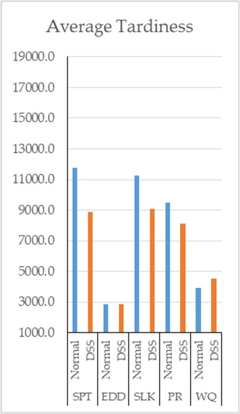
Mathematics 2019, 7, 278                                                                                      6 of 19
Mathematics 2019, 7, x FOR PEER REVIEW                                                                       6 of 20

     When scheduling the jobs according to a specific rule (as         (as described
                                                                           described below), a priority
                                                                                                  priority value is
calculated for
calculated  foreach
                 eachjob
                       jobininthe
                               thequeue.
                                   queue.Later,
                                           Later,thethe
                                                      jobjob with
                                                           with thethe  smallest
                                                                    smallest      or the
                                                                              or the     largest
                                                                                     largest valuevalue  is selected
                                                                                                    is selected and
and assigned
assigned  to thetoworkstation.
                   the workstation.
     Dispatching rules
     Dispatching    rulescancanbe
                                beclassified
                                   classifiedininvarious
                                                  various    ways.
                                                           ways.    The
                                                                  The    rules
                                                                       rules    which
                                                                             which  areare  assigned
                                                                                        assigned       according
                                                                                                   according      to
                                                                                                              to the
the conditions
conditions       in workshop
            in the  the workshop can can  be grouped
                                     be grouped    under under
                                                            threethree
                                                                   majormajor classes
                                                                          classes      as given
                                                                                  as given       in Figure
                                                                                            in Figure  2. 2.

                               Figure 2. Dispatching rules in job-shop scheduling.
                               Figure 2. Dispatching rules in job-shop scheduling.
     Rules Based on the Job: According to the dispatching rules based on the job, the assignment is
      Rules Based on the Job: According to the dispatching rules based on the job, the assignment is
done by ignoring the interdependencies between the workstations. Priorities for jobs are determined
done by ignoring the interdependencies between the workstations. Priorities for jobs are determined
with respect to some of the attributes and values of the job, such as arrival times, processing times,
with respect to some of the attributes and values of the job, such as arrival times, processing times,
due dates, etc. Then, the job having the smallest priority value is selected first. Rules such as SPT, EDD,
due dates, etc. Then, the job having the smallest priority value is selected first. Rules such as SPT,
SLACK, and PR can be classified as rules based on the Job.
EDD, SLACK, and PR can be classified as rules based on the Job.
     Rules Based on the Job-Shop: In order to increase the efficiency in smart factories of the
      Rules Based on the Job-Shop: In order to increase the efficiency in smart factories of the future,
future, the components and subsystems must be integrated with each other. For this integration,
the components and subsystems must be integrated with each other. For this integration, machines
machines should work intelligently by communicating with other machines. In such a system, process
should work intelligently by communicating with other machines. In such a system, process
monitoring can be carried out in a comprehensive and effective manner using simultaneous data from
monitoring can be carried out in a comprehensive and effective manner using simultaneous data
the machines and other units. The machines will be able to plan their own production resources. Thus,
from the machines and other units. The machines will be able to plan their own production resources.
lean manufacturing and just-in-time manufacturing could be realized.
Thus, lean manufacturing and just-in-time manufacturing could be realized.
     Until recently, real-time data to show the status of the job-shop were not available. Therefore,
      Until recently, real-time data to show the status of the job-shop were not available. Therefore,
dispatching rules that can update the priority values of the jobs dynamically and autonomously were
dispatching rules that can update the priority values of the jobs dynamically and autonomously were
not very common. Work load in next queue (WinQ) rule is a good example for this new class of rules.
not very common. Work load in next queue (WinQ) rule is a good example for this new class of rules.
     Hybrid Rules: Hybrid rules are formed by combining two or more dispatching rules. In this case,
      Hybrid Rules: Hybrid rules are formed by combining two or more dispatching rules. In this
a priority value is calculated based on the priority values of these rules. This value is used to specify
case, a priority value is calculated based on the priority values of these rules. This value is used to
the job to be assigned.
specify the job to be assigned.
Dispatching Rules Considered in the Study
3.1. Dispatching Rules Considered in the Study
     The DSS moves in whenever the number of jobs waiting in the queue of any workstation in
     The DSSfalls
the job-shop     moves   in whenever
                      to the             the number
                             critical value   of one. of
                                                      Thejobs waiting
                                                            DSS        in the queue
                                                                 is designed           of anythe
                                                                               to increase     workstation in the
                                                                                                 performance   of
job-shop   falls  to the  critical  value  of  one. The   DSS  is  designed   to  increase   the performance
dispatching rules in dynamic scheduling using real time data. For this purpose, five dispatching rules         of
dispatching    rules in dynamic    scheduling   using real time data. For  this purpose,   five dispatching
with good job-shop performances, which were demonstrated in the literature, are selected in order to        rules
with good
compare   thejob-shop   performances,
                performances              which were
                                of the dispatching     demonstrated
                                                     rules              in the literature,
                                                           with and without     the DSS. are selected in order
to compare    the  performances     of the dispatching  rules with  and  without
     These rules are explained in this section. Notations are given in Table       the1.DSS.
     These rules are explained in this section. Notations are given in Table 1.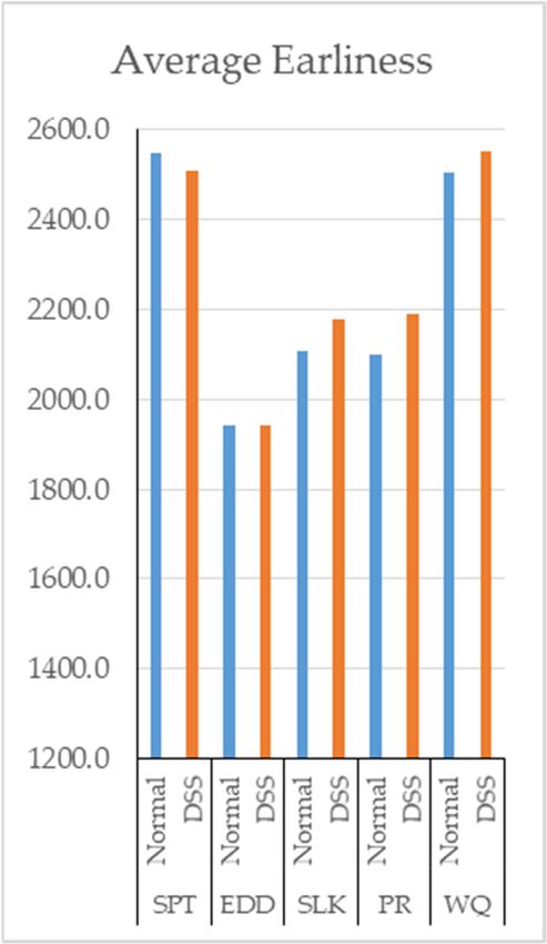
Mathematics 2019, 7, 278                                                                                       7 of 19

                                      Table 1. Notations for Dispatching Rules.

            πi,j   Priority value in the jth operation of job       ni     Total number of operations of job
            di     Due date of job                                  Ai     Arrival time of job
                                                                           The time when a dispatching
            Pi,j   Processing time of the jth operation of job      t
                                                                           decision is needed
                                i: Job Index; j: Operation Index; k: Current Operation Step.

    Smallest Processing Time (SPT): In this rule, the priority value is the processing time at the
workstation. Between the jobs waiting in the queue, the job with the smallest processing time in the
queue is selected as the job to be processed first.

                                                       πi,k = Pi,k ,                                              (1)

     Earliest Due Date (EDD): In this rule, the priority value of jobs is the due date. Between the
jobs waiting in the queue, the job with the earliest due date in the queue is selected as the job to be
processed first.
                                              πi,k = di ,                                            (2)

    Shortest Slack Time (SLACK): In this rule, the priority value is obtained by subtracting the
remaining total processing time from the remaining time to due date. Between the jobs waiting in the
queue, the job with the smallest priority value in the queue is selected as the job to be processed first.
                                                             "             #
                                                                    ni
                                              πi,k = di − t + ∑ Pi,j ,                                            (3)
                                                                   j=k

     Priority Ratio (PR): In this rule, the priority value is obtained by dividing the remaining time
until the due date by the remaining total processing time. Between the jobs waiting in the queue,
the job with the smallest priority value in the queue is selected as the job to be processed first.
                                                                    ni
                                               πi,k = (di − t) / ∑ Pi,j ,                                         (4)
                                                                    j=k

      Work load in the next Queue (WinQ): Apart from these static dispatching rules, a dispatching
rule that can be adapted to dynamic environments is presented below. The rule WinQ was proposed
by Holthaus and Rajendran [32]. This rule determines the priority value of a job by considering the
conditions of the job-shop. In this rule, priority value is obtained by looking at total processing times
of all jobs in the next workstation, depending on a job’s route. Among the jobs waiting in the current
queue, the job with the smallest priority value is selected as the next job to be processed. They reported
that use of this rule minimizes the average flow time. In cases when the utilization of a job-shop is
high, the due dates are determined in A narrow range. This rule also minimizes the tardiness of the
jobs and the ratio of the tardy jobs.

4. Decision Support System
     A DSS is a computerized information system used to support decision-making in an organization.
The DSS proposed in this study can be considered as an automated DSS [33], which automatically
collects data from the job-shop, analyze the data, and intervenes in the processing order of the jobs if
necessary. In other words, it continuously monitors operations, seeks opportunities to increase the
job-shop performance, and formulates a better processing order and implements it.
     When dispatching rules are used for scheduling, the rule to be applied is determined before the
system starts running and no modification are allowed at any time. In this study, we propose a new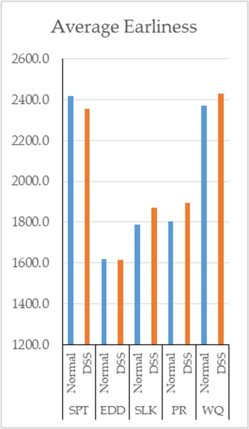
Mathematics 2019, 7, 278 8 of 19
Mathematics 2019, 7, x FOR PEER REVIEW 8 of 20
dynamic approach where priority of the jobs can be updated in real time depending on the information
information
on the current on the current
status of thestatus of the workstations.
workstations. The goal isThe goal is tothe
to improve improve the performance
performance of theby
of the system
system by decreasing
decreasing idle time idle time
in the in the workstations.
workstations.
To collect real-time data
To collect real-time data from from the the
workstations,
workstations,the status of the of
the status machines (idle, busy),
the machines (idle,queue
busy),
lengths,
queue lengths, and the property of the jobs in the queue (remaining processing time, time,
and the property of the jobs in the queue (remaining processing time, processing due
processing
date etc.)
time, duearedate
sentetc.)
to theare
management
sent to the module of the module
management system. When
of the the information
system. When is received
the by theis
information
DSS, the system makes necessary modifications in the queue order if it is
received by the DSS, the system makes necessary modifications in the queue order if it is needed. needed. As soon as theAs
number of jobs waiting in a queue at any workstation falls to a critical level (in this
soon as the number of jobs waiting in a queue at any workstation falls to a critical level (in this study study this critical
level
this is chosen
critical as one),
level the DSS
is chosen examines
as one), the DSS allexamines
the preceding
all theworkstations to detect the
preceding workstations to jobs that
detect thewill
jobs
bethat
sentwill
to this workstation. Then, it determines the job with the highest priority
be sent to this workstation. Then, it determines the job with the highest priority numbernumber according to
the active dispatching
according to the active rule. Finally, therule.
dispatching DSSFinally,
places this
the job
DSStoplaces
the first order
this job toof the
the first
its queue
ordersoofthat
the itits
will
queue so that it will be first one to be processed when the station becomes idle. Thus, idle times willinbe
be first one to be processed when the station becomes idle. Thus, idle times will be avoided
the workstations
avoided as much as possible.
in the workstations as much as possible.
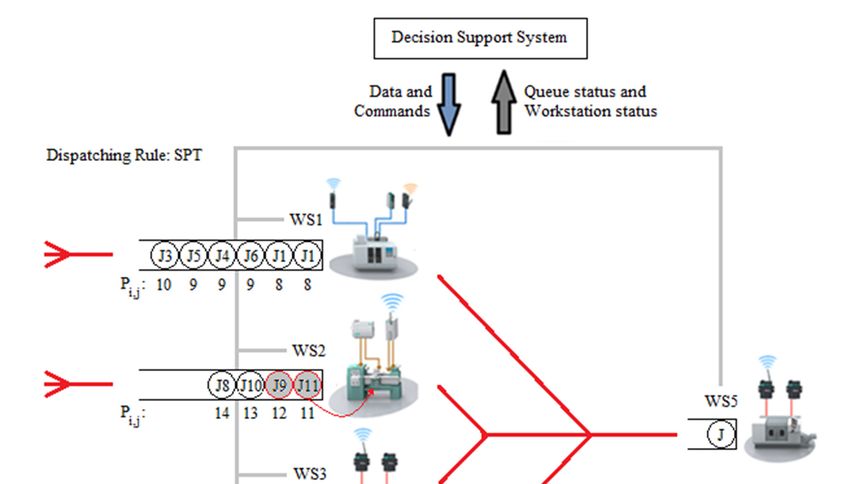
ToTo explain how this approachworks,
explain how this approach works,an anexample
exampleisispresented
presentedininFigure
Figure3.3.
Anexample
Figure3.3.An
Figure exampleofofhow
howa aDecision
DecisionSupport
SupportSystem
System(DSS)
(DSS)works.
works.
In this example, suppose that at a specific time point, Figure 3 illustrates the current queue order in
In this example, suppose that at a specific time point, Figure 3 illustrates the current queue order
the system. Further, suppose that the DSS works under the SPT rule to schedule the jobs in the system
in the system. Further, suppose that the DSS works under the SPT rule to schedule the jobs in the
and the number of jobs in the queue of WS5 drops to one (a critical level). When the route information
system and the number of jobs in the queue of WS5 drops to one (a critical level). When the route
is examined, it is determined that WS1, WS2, WS3, and WS4 are the preceding workstations that could
information is examined, it is determined that WS1, WS2, WS3, and WS4 are the preceding
send the jobs either to WS5 or to other workstations, depending on the route of the jobs. Jobs that
workstations that could send the jobs either to WS5 or to other workstations, depending on the route
could be processed in the preceding workstations of WS5 are given below:
of the jobs. Jobs that could be processed in the preceding workstations of WS5 are given below: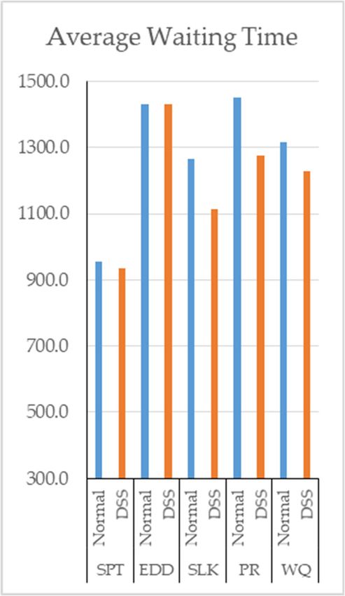
Mathematics 2019, 7, 278                                                                                         9 of 19

     WS1 = {J1, J2, J3, J4, J5, J6}
     WS2 = {J7, J8, J9, J10, J11, J12, J13, J14}
     WS3 = {J3, J4, J5, J6, J7, J10, J13, J14, J15, J16, J17, J18, J19, J20}
     WS4 = {J1, J2, J3, J4, J5, J6, J7, J8, J9, J10, J13, J14, J15, J16, J17, J18, J19, J20}

     The jobs that are underlined in the lists are the ones that will be sent to WS5 after processed in
their current workstations. The other jobs will be sent to other workstations according to their routes.
The routes and precedence orders can be seen in Table 2 in the Section 5.
     The DSS first determines which of these jobs could be processed next in WS5 by checking WS1,
WS2, WS3, and WS4. The job numbers colored in gray in each queue in Figure 3 are the jobs that
could be processed in WS5, namely J4, J9, and J11. Among them, J4 is selected since it has the smallest
processing time (according to SPT). This job is in the WS4 queue, and hence will be processed in the
WS4 as soon as it becomes idle.

                                Table 2. Routes and Unit Processing Times of Parts.

              Operation 1   Operation 2    Operation 3     Operation 4    Operation 5     Operation 6    Operation 7
   Part 1       WS1(8)        WS2(12)        WS5(12)         WS4(7)         WS7(13)
   Part 2       WS1(8)        WS5(19)        WS4(12)         WS8(15)        WS6(10)
   Part 3       WS1(10)       WS4(8)          WS3(6)         WS6(8)          WS9(9)
   Part 4       WS1(9)        WS6(10)        WS3(10)         WS4(10)        WS5(14)            WS9(8)     WS10(10)
   Part 5       WS1(9)        WS4(10)         WS3(8)         WS5(15)        WS10(11)           WS9(5)
   Part 6       WS1(9)        WS2(10)         WS3(8)         WS4(11)        WS5(10)            WS6(9)     WS10(14)
   Part 7       WS2(13)       WS3(11)        WS4(10)         WS5(16)        WS8(18)            WS9(9)
   Part 8       WS2(14)       WS4(14)        WS5(13)         WS7(14)        WS8(18)            WS9(10)
   Part 9       WS2(12)       WS5(9)         WS4(11)         WS7(16)        WS10(14)
   Part 10      WS2(13)       WS3(9)          WS4(7)         WS8(14)        WS7(14)            WS6(10)
   Part 11      WS2(11)       WS5(10)        WS6(10)
   Part 12      WS2(10)       WS5(11)        WS4(10)         WS8(17)        WS9(12)
   Part 13      WS2(12)       WS5(12)        WS4(10)         WS3(8)          WS6(8)            WS9(7)
   Part 14      WS2(13)       WS5(10)        WS4(11)         WS3(8)          WS6(9)            WS7(17)    WS10(12)
   Part 15      WS3(10)       WS6(9)         WS4(11)         WS8(17)        WS7(15)
   Part 16      WS3(9)        WS5(10)         WS4(9)         WS7(18)
   Part 17      WS3(8)        WS4(7)         WS8(15)
   Part 18      WS3(9)        WS5(10)        WS4(10)         WS6(8)
   Part 19      WS3(8)        WS4(9)         WS7(15)         WS6(11)
   Part 20      WS3(8)        WS5(11)         WS4(9)         WS8(15)        WS6(12)

5. The Simulation Model
     A simulation model for a job-shop production environment, developed in Arena, is used to
assess the effects of the proposed DSS. The virtual job-shop environment starts the production with
the arrival of a demand for a job. It is assumed that there is a continuous dynamic job demand
arrival. Manufacturing takes place at 10 workstations and real-time data can be obtained from them.
Each workstation has a different numbers of machines. The representative layout of this job-shop
environment is shown in Figure 4.
     The purpose of this simulation study is to analyze the effects of introducing the DSS into a job-shop
environment that is normally working with some dispatching rule. In this simulation, some real-life
phenomena, such machine failures will not be considered since they are not considered to have a
significant influence on the performance of the DSS. The simulation model was formed under the
following assumptions: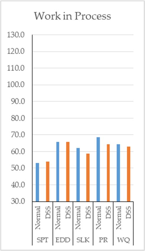
workstation has a different numbers of machines. The representative layout of this job-shop
environment is shown in Figure 4.
     The purpose of this simulation study is to analyze the effects of introducing the DSS into a job-
shop environment that is normally working with some dispatching rule. In this simulation, some
real-life phenomena,
Mathematics 2019, 7, 278 such machine failures will not be considered since they are not considered  10 of to
                                                                                                           19
have a significant influence on the performance of the DSS. The simulation model was formed under
the following assumptions:
 •   Each order has only a single type of job.
•    Each order has only a single type of job.
 •   A job cannot be divided and requires different operations in different workstations. For this
•    A job cannot be divided and requires different operations in different workstations. For this
     reason, two operations of the same job cannot be processed at the same time.
     reason, two operations of the same job cannot be processed at the same time.
 •   Previous operations of a job must be completed to start a new operation.
•    Previous operations of a job must be completed to start a new operation.
••   Jobs
     Jobs cannot
            cannot be be cancelled.
                         cancelled. Each
                                     Each job
                                           job should
                                               should be
                                                       be processed
                                                          processed until
                                                                     until it
                                                                            it is
                                                                               is completed.
                                                                                  completed.
••   Machine     failures  have   been
     Machine failures have been ignored.ignored.
••   Quality
     Quality control
               control operations
                          operations are
                                      are ignored.
                                           ignored. Thus,
                                                     Thus, waste
                                                           waste parts
                                                                  parts do
                                                                         do not
                                                                             not occur.
                                                                                  occur.
••   The  time   required    to  move parts   between workstations   is also  ignored.
                              to move parts between workstations is also ignored.
••   Queues in front of workstations
                              workstations are
                                             are allowed.
                                                 allowed.
•    Jobs can wait in    in aa queue
                                queue for
                                       for the
                                            the machine
                                                machine toto become
                                                              become idle.
                                                                       idle. On the other hand, machines in
     workstations can  can remain
                            remain idle.
                                    idle.

                               Figure 4. Representative Job-shop Layout Plan.
                               Figure 4. Representative Job-shop Layout Plan.
     The routes and the unit processing times of the 20 parts to be produced is obtained from a
company that produces spare parts. Data about parts are given in Table 2. It is assumed that the
incoming job order can be for any product (each of the 20 parts are equally likely) and the size of the
incoming order can be any value between 10 and 30.
     When jobs arrive the system, they are directed to the first workstation on their route. If the
targeted workstation is idle, the process starts, otherwise it is kept in the queue. If there are jobs
waiting in the queue, a priority value for each job is calculated based on the dispatching rule. Then,
the job with the highest or lowest priority is selected. Jobs that are processed in a workstation are
directed to their next workstation in their route. The processing of a job is completed when all the
workstations on the route are visited.

5.1. Determining the Best Working Conditions of the System
      The simulation model was set up to represent a job-shop with realistic due dates and a realistic
number of machines in workstations, so that job flows are made as smooth as possible without
serious bottlenecks.
      In order for this setup, the simulation model of the designed system was tested according to
the first-in-first-out (FIFO) dispatching rule under exponential job arrival times with various means.
The results were compared in terms of the capacity utilization rates of the workstations and the length
of the queue formed in front of each workstation (whether the queue lengths increase continuously or
cause bottlenecks). It was observed that a mean value of 65 produced satisfactory results. The model
was tested with smaller and larger mean values as will be discussed in Section 5.2.
      Since some performances criteria are directly related to due dates, due dates were determined as
realistically as possible. In real life, due dates are usually set by customers and jobs can have a wide or
Mathematics 2019, 7, 278 11 of 19
narrow due-date interval depending on how urgent the production is. This must include a coincidence
factor that considers the nature of the orders received (normal or urgent) in determining the due date.
In our study, a new equation (Equation (5)) was used to determine the due date.
To obtain due dates (di ), the proposed model was again run according to the FIFO dispatching
rule and the amount of time spent in the system by each job was found. Next, the processing time
of each job was subtracted from the amount of time the job spends in the system to find the waiting
time of the job in the system. Then the waiting time was divided to the processing time to obtain a
ratio. This ratio shows the percentage of processing time to waiting time. An analysis of these ratios
showed that their distribution can be approximated by an exponential distribution except for the fact
that it does not start from zero. It is known that exponential distribution can produce values between
zero and infinity. Suppose that we obtained zero waiting time from this distribution. This means that
the due date of the job would be equal to its arrival time plus its processing time. However, in the
job-shop, this due date is not realistic since the job with this due date would probably be a tardy job.
To avoid this, we add a constant term (1 + h) to the formula presented in Equation (5) to produce
more realistic due dates. We defined a tightness factor h to transform the value obtained from the
exponential distribution.
Accordingly, the newly proposed due date generation rule (Equation (5)) is as follows;
20 10
di = Ai + ( ∑ ∑ Pi,j ) · (1 + h + Expo(µ)), (5)
i =1 j =1
where di represents the i-th due date and h represents the tightness factor. We determined that h
should be 1.5 after trial and error. Below this value, we observed many tardy jobs. Finally, the µ value
is set to 1.5.
Before testing our scenarios, the simulation model was run by considering different numbers of
machines at each workstation to determine the right number of machines at each workstation. Some
runs according to different machine combinations (X, Y, and Z) at each workstation were shown in
Table 3. Results showed that best machine combination is the Z, with one machine in WS1, WS9,
and WS10, three machines in WS4 and WS5, and two machines in the rest of the stations, which
were best in terms of average workstation utilization, average waiting time, and average number of
parts waiting.
5.2. Scenarios
The simulation model was run under three different scenarios:
• Scenario 1: Exponential distribution with a mean of 62 is used to represent arrivals of a fast order
rate which overloads the job-shop.
• Scenario 2: Exponential distribution with a mean of 65 is used to represent arrivals of a moderate
order rate for a balanced structure.
• Scenario 3: Exponential distribution with a mean of 68 is used to represent arrivals of a slower
order rate which causes a more relaxed job-shop.
These three scenarios were run by considering SPT, EDD, SLACK, PR, and WinQ dispatching
rules in a job-shop supported by the DSS. Two situations in terms of control are considered: with DSS
and without DSS (Normal).
In each scenario, 5000 orders are received randomly according to the arrival speed and a simulation
run is completed when all the orders were produced. The fact that the same orders were created at
the same time for each scenario enabled one-to-one comparisons. Thus, more realistic evaluations
were achieved.Mathematics 2019, 7, 278 12 of 19
Table 3. Results of some runs according to different machine combinations.
X: 1-1-2-2-2-2-2-1-1-1 Y: 1-2-2-3-2-2-2-2-1-1 Z: 1-2-2-3-3-2-2-2-1-1
Average Average Average Average Average Average
Average Average Average
Number Workstation Number Workstation Number Workstation
Waiting Time Waiting Time Waiting Time
Waiting Utilization Waiting Utilization Waiting Utilization
WS1 0.81 344 0.42 1.13 344 0.58 1.56 344 0.80
WS2 506.64 132,869 0.92 2.34 438 0.65 3.20 438 0.88
WS3 0.55 98 0.48 3.19 407 0.67 6.26 582 0.92
WS4 118.81 15,946 0.73 0.94 90 0.68 3.54 248 0.94
WS5 15.46 2638 0.71 520.83 63443 0.99 3.52 313 0.91
WS6 0.21 43 0.46 0.63 94 0.64 2.78 301 0.88
WS7 0.13 42 0.44 0.40 92 0.62 1.41 237 0.85
WS8 210.25 68,121 0.99 0.65 149 0.70 6.41 1081 0.96
WS9 0.16 58 0.47 0.57 148 0.66 3.03 572 0.90
WS10 0.35 172 0.49 0.58 204 0.69 6.01 1548 0.94Mathematics 2019, 7, 278 13 of 19
5.3. Results of Scenarios
To reduce the effects of randomness on results, the simulation model was run under 50 replications
for each scenario and the averages of performance criteria were obtained.
The scenarios were compared based on the following performance criteria:
• Number of tardy jobs: The timely delivery of orders in the job-shop is of great importance both
for customer satisfaction and penalty costs.
• Average waiting time in queue (Avg. waiting time): This criterion attempted to determine whether
the waiting periods in the system decreased or not.
• Utilization of the workstations (Avg. utilization): This criterion attempted to determine whether
the scenarios increase the efficiency of the system.
• Work in Process (Wip): This criterion attempted to determine whether the scenarios increase the
work load within the system.
• Average tardiness (Avg. tardiness): Considering only the number of tardy jobs may lead to
incorrect results. It will be better to examine delays together with the average deviations from the
due date.
• Average earliness (Avg. earliness): In addition to the late completion of the jobs, it is not desirable
to complete jobs early due to inventory holding costs. To avoid these costs jobs should be
completed as close as possible to their corresponding due dates.
The simulation results with respect to these performance criteria, are given in the Appendix A.
The graphical
Mathematics comparisons of REVIEW
2019, 7, x FOR PEER the scenarios based on the criteria are shown in Figures 5–10. 14 of 20
Expo(62) Expo(65) Expo(68)
Figure
Figure 5. 5. Averageutilization.
Average utilization.
SinceSince the DSS
the DSS basically
basically controls
controls the situation
the situation of each
of each workstation
workstation andand updates
updates thethe sequence
sequence ofofthe
jobs according to the dispatching rule, an increase in average utilization of each scenario is observedisin
the jobs according to the dispatching rule, an increase in average utilization of each scenario
observed in Figure 5.
Figure 5.Expo(62) Expo(65) Expo(68)
Figure 5. Average utilization.
Since the DSS basically controls the situation of each workstation and updates the sequence of
the jobs
Mathematics 2019,according
7, 278 to the dispatching rule, an increase in average utilization of each scenario is 19
14 of
observed in Figure 5.
Expo(62) Expo(65) Expo(68)
Figure
Figure 6. 6. Average
Average waitingtime.
waiting time.
The proposed
The proposed approach
approach alsoalso leads
leads to to a decreaseononaverage
a decrease averagewaiting
waiting time
time of
ofthe
thejobs
jobsininthe system;
the system;
this is in line with the increase in utilization rates. On the other hand, the amount of decrease
this is in line with the increase in utilization rates. On the other hand, the amount of decrease observed observed
in each scenario was different. The sharpest decrease in Figure 6 was observed in Scenario 1.
in each scenario
Mathematics was
2019, 7, xdifferent. The sharpest decrease in Figure 6 was observed in Scenario 1. 15 of 20
FOR PEER REVIEW
Expo(62) Expo(65) Expo(68)
Figure
Figure 7. Work
7. Work in in Process.
Process.
Because
Because of theofdecrease
the decrease in the
in the average
average waiting
waiting times,the
times, thenumber
numberof
of jobs
jobs in
in the
the system
systemdecreased
decreased
except for the cases in which the SPT rule is
except for the cases in which the SPT rule is used. used.Expo(62) Expo(65) Expo(68)
Figure 7. Work in Process.
MathematicsBecause of the decrease in the average waiting times, the number of jobs in the system decreased
2019, 7, 278 15 of 19
except for the cases in which the SPT rule is used.
Expo(62) Expo(65) Expo(68)
Figure
Figure 8. 8. NumberofofTardy
Number TardyJobs.
Jobs.
AfterAfter the results
the results presented
presented in Figure
in Figure 8 were8evaluated,
were evaluated,
we did wenot did not observe
observe a significant
a significant difference
in terms of tardy jobs. This is probably because of the randomness in the due dates and theand
difference in terms of tardy jobs. This is probably because of the randomness in the due dates factthe
that
fact that the
Mathematics EDD,
2019, thePEER
7, x FOR SLACK, and the PR dispatching rules consider the due dates of jobs. 16
REVIEW Onofthe
20
the EDD, the SLACK, and the PR dispatching rules consider the due dates of jobs. On the other hand,
a decrease is observed
other hand, a decreasewhen the WinQ
is observed whenrule isWinQ
the used since
rule isthis
usedrule is this
since based
ruleon the amount
is based of jobs in
on the amount
the system.
of jobs in the system.
Expo(62) Expo(65) Expo(68)
Figure
Figure 9. 9.Average
AverageTardiness.
Tardiness.
A decrease in the number of tardy jobs was not observed when dispatching rules based on due
date (see Figure 9). However, for the cases in which WinQ is considered, a decrease in the average
waiting times does not occurred because of the increase in the average utilization of workstations.Mathematics 2019,Expo(62)
7, 278 Expo(65) Expo(68) 16 of 19
Figure 9. Average Tardiness.
A decrease in the number of tardy jobs was not observed when dispatching rules based on due
A decrease in the number of tardy jobs was not observed when dispatching rules based on due
date (see Figure 9). However,
date (see Figure for for
9). However, thethe
cases in in
cases which
whichWinQ
WinQisisconsidered,
considered, aa decrease inthe
decrease in theaverage
average
waiting timestimes
waiting doesdoes
not occurred because
not occurred of the
because increase
of the ininthe
increase theaverage
averageutilization
utilization of workstations.
of workstations.
Expo(62) Expo(65) Expo(68)
Figure
Figure 10.10. Average
Average Earliness.
Earliness.
After the results in Figure 10 were examined, an increase in average earliness was observed,
except for the case in which SPT rule was used. This was an expected outcome since an increase in
utilization and a decrease in waiting times is already observed.
6. Results and Discussion
The DSS proposed in this study aims at increasing the performance of dispatching rules in
dynamic scheduling using real time data, hence increasing the overall performance of the job-shop.
The DSS can work with all dispatching rules. This study shows that a DSS that fed with real time data
from a job-shop can help improve several performance criteria. This can be achieved in job-shops
equipped with Industry 4.0 hardware and software. The proposed approach improves the performance
of a system in terms of number of tardy jobs, average waiting time in queue, average utilization of
the workstations, work in process, average tardiness, and earliness as it is discussed in the previous
section. As expected, machine utilization increased and thus waiting times in the system and the
amount of work-in-process decreased using the DSS.
If the big data collected in real data could be analyzed, inner dynamics between the components of
the system could be solved. Understanding the production systems better could help the researchers to
develop advanced DSS and the decision makers to make better decisions. Controlling the production
environment using real time data, could also help researchers to model the system without making
any assumptions. This approach could close the gap between theory and practice and result in realistic
solutions. Moreover, it would be possible to validate actual processing times of jobs considering past
data about jobs.
Data stored in dynamic databases could also be processed with data mining techniques in order
to determine potential problems in the production; to obtain rules that could improve the efficiency of
production; to generate rules to effectively control the production; to develop automation based onMathematics 2019, 7, 278 17 of 19
work intelligence; and to improve quality of products and even to design a production management
system that could improve itself.
Since the analysis of this big data would help predict the behavior of the system under different
conditions, any subsystem could easily integrate into this system. The integration of artificial intelligence
or machine learning based subsystems could constitute smart factories of the future. In this respect,
this study demonstrates, at a theoretical level, the benefits to be gained by such subsystem integrations,
though technological integration in a real job-shop may take substantial time and effort.
7. Conclusions
In this study, we considered a dynamic job-shop where job lists are updated dynamically because
of continuous arrival of new orders. In future studies, various cases including machine breakdowns,
cancellation of orders, and quality control processes should be considered. Handling these more
complex cases requires collection of more data with an enriched nature. This will enable the decision
makers to control the production better by considering real time management of stochastic disturbances
to the system. However, to analyze and evaluate this big data better, advanced decision support
systems supported by efficient strategies are needed.
Author Contributions: This paper carried out by all authors equally. Conceptualization, O.O.E. and B.B.;
Data curation, A.F.I.; Formal analysis, A.F.I.; Investigation, A.A.; Methodology, A.K.T.; Project administration,
G.S.D.; Software, A.K.T.; Supervision, A.A.; Validation, A.F.I., G.S.D., and B.B.; Visualization, O.O.E.
Funding: This research received no external funding.
Conflicts of Interest: The authors declare no conflict of interest.
Appendix A
SPT EDD SLACK PR WinQ
Number of tardy jobs 714.6 3333.8 1070.9 1386.3 2693.1
Avg. waiting Time 954.3 1430.8 1266.7 1452.2 1317.0
Expo(62)
Avg. utilization 90.267% 90.701% 90.619% 90.856% 90.786%
Work in process 83.9 118.3 106.7 121.6 110.8
Avg. tardiness 20570.1 5483.9 16681.9 16124.5 6956.0
Avg. earliness time 2281.4 1307.7 1416.2 1453.0 2223.2
Number of tardy jobs 492.7 1614.9 525.3 802.2 1669.2
Avg. waiting Time 548.9 750.9 690.8 782.4 723.4
Expo(65)
Normal
Avg. utilization 89.127% 89.171% 89.167% 89.309% 89.270%
Work in process 53.0 65.6 62.1 68.5 64.3
Avg. tardiness 11762.6 2830.6 11249.4 9468.0 3910.0
Avg. earliness time 2416.6 1617.9 1785.9 1803.3 2372.1
Number of tardy jobs 322.4 492.4 243.8 450.0 972.0
Avg. waiting Time 334.9 420.9 404.4 458.1 419.3
Expo(68)
Avg. utilization 86.291% 86.271% 86.270% 86.353% 86.353%
Work in process 37.6 42.7 41.8 45.3 42.8
Avg. tardiness 6445.9 1361.2 6730.3 5250.2 2065.9
Avg. earliness time 2548.1 1942.7 2109.5 2101.5 2504.0
Number of tardy jobs 937.6 3333.8 1132.6 1444.2 2542.5
Avg. waiting Time 936.1 1430.1 1115.3 1277.1 1230.1
Expo(62)
Avg. utilization 90.871% 90.703% 90.849% 91.003% 90.864%
Work in process 85.3 118.3 99.2 111.5 107.8
Avg. tardiness 14996.8 5481.3 13636.3 13190.4 7138.9
Avg. earliness time 2183.4 1305.8 1465.3 1491.7 2261.2Mathematics 2019, 7, 278 18 of 19
Number of tardy jobs 620.0 1612.3 556.1 811.5 1481.2
Avg. waiting Time 534.5 750.6 605.3 691.0 663.2
Expo(65)
Avg. utilization 89.356% 89.170% 89.284% 89.402% 89.376%
DSS
Work in process 54.0 65.6 58.7 64.5 62.9
Avg. tardiness 8863.9 2833.7 9087.0 8112.7 4505.2
Avg. earliness time 2354.0 1615.3 1868.9 1893.8 2429.7
Number of tardy jobs 385.3 489.0 268.1 459.0 887.7
Avg. waiting Time 317.6 420.9 357.1 400.4 381.3
Expo(68)
Avg. utilization 86.383% 86.271% 86.359% 86.407% 86.387%
Work in process 38.0 42.7 40.5 43.2 42.1
Avg. tardiness 4857.4 1398.7 5368.9 4437.0 2493.2
Avg. earliness time 2509.7 1943.3 2176.9 2192.2 2554.3
References
1. Ersöz, O.Ö.; Türker, A.K. Simultaneous production planning & control with current workstation loading.
Manas J. Soc. Stud. 2016, 5, 5.
2. Elhüseyni, M. Hipotetik Bir Tekstil Atölyesinin Dinamik Çizelgelenmesinde Yollama Kurallarının Benzetim Tekniğiyle
Analizi; İstanbul Teknik Üniversitesi, Fen Bilimleri Enstitüsü: Istanbul, Turkey, 2012.
3. Azadeh, A.; Negahban, A.; Moghaddam, M. A hybrid computer simulation-artificial neural network
algorithm for optimisation of dispatching rule selection in stochastic job shop scheduling problems. Int. J.
Prod. Res. 2012, 50, 551–566. [CrossRef]
4. Larsen, R.; Marco, P. A framework for dynamic rescheduling problems. Int. J. Prod. Res. 2018, 57, 1–18.
[CrossRef]
5. Banks, J.; Carson, J.S.; Nelson, B.L.; Nicol, D.M. Discrete-Event System Simulation, 3rd ed.; Printice Hall: Upper
Saddle River, NJ, USA, 2001; ISBN 978-0136062127.
6. Law, A.M.; Kelton, W.D. Simulation Modeling and Analysis, 2nd ed.; McGraw-Hill International: New York,
NY, USA, 1991; ISBN 978-0073401324.
7. Koruca, H.İ.; Özdemir, G.; Aydemir, E.; Çayırlı, M. Bir simülasyon Yazılımı için Esnek İş Akış Planı Editörü
Geliştirilmesi; İşlemlerin Gantt Şemasında Çizelgelenmesi. J. Fac. Eng. Archit. Gazi Univ. 2010, 25, 77–81.
8. Zhong, R.Y.; Chen, C.; Huang, G.Q. Big Data Analytics for Physical Internet-based intelligent manufacturing
shop floors. Int. J. Prod. Res. 2015, 55, 2610–2621. [CrossRef]
9. Marinho, R.; Bragança, A.; Ramos, C. Decision Support System for Dynamic Production Scheduling.
In Proceedings of the 1999 IEEE International Symposium on Assembly and Task Planning (ISATP’99)
(Cat. No. 99TH8470), Porto, Portugal, 24–24 July 1999; pp. 424–429.
10. Aydın, M.E.; Öztemel, E. Dynamic job-shop scheduling using reinforcement learning agents. Robot. Auton.
Syst. 2000, 33, 169–178. [CrossRef]
11. Li, L.; Chang, Q.; Ni, J.; Biller, S. Real time production improvement through bottleneck control. Int. J. Prod.
Res. 2009, 47, 6145–6158. [CrossRef]
12. Heilala, J.; Montonen, J.; Jarvinen, P.; Kivikunnas, S.; Maantila, M.; Sillanpaa, J.; Jokinen, T. Developing
Simulation-Based Decision Support Systems for Customer-driven Manufacturing Operation Planning.
In Proceedings of the 2010 Winter Simulation Conference, Baltimore, MD, USA, 5–8 December 2010;
pp. 3363–3375.
13. Madhavi, I.; Shirazi, B. A Review of Simulation-based Intelligent Decision Support System Architecture for
the Adaptive Control of Flexible Manufacturing Systems. J. Artif. Intell. 2010, 3, 201–219. [CrossRef]
14. Sharma, P.; Jain, A. Analysis of dispatching rules in a stochastic dynamic job shop manufacturing system
with sequence-dependent setup times. Front. Mech. Eng. 2014, 9, 380–389. [CrossRef]
15. Sharma, P.; Jain, A. New setup-oriented dispatching rules for a stochastic dynamic job shop manufacturing
system with sequence-dependent setup times. Concurr. Eng. Res. Appl. 2016, 24, 58–68. [CrossRef]You can also read