Coordination of Power-System Stabilizers and Battery Energy-Storage System Controllers to Improve Probabilistic Small-Signal Stability Considering ...
←
→
Page content transcription
If your browser does not render page correctly, please read the page content below
applied
           sciences
Article
Coordination of Power-System Stabilizers and Battery
Energy-Storage System Controllers to Improve
Probabilistic Small-Signal Stability Considering
Integration of Renewable-Energy Resources
Samundra Gurung † , Sumate Naetiladdanon *,† and Anawach Sangswang †
 Department of Electrical Engineering, King Mongkut’s University of Technology Thonburi (KMUTT),
 Bangkok 10140, Thailand; samundra.g@mail.kmutt.ac.th (S.G.); anwach.san@kmutt.ac.th (A.S.)
 * Correspondence: sumate.nae@kmutt.ac.th
 † These authors contributed equally to this work.

 Received: 10 February 2019; Accepted: 10 March 2019; Published: 15 March 2019

 Featured Application: Power-system-controller tuning.

 Abstract: This paper proposes a probabilistic method to obtain optimized parameter values
 for different power-system controllers, such as power-system stabilizers (PSSs) and battery
 energy-storage systems (BESSs) to improve probabilistic small-signal stability (PSSS) considering
 stochastic output power due to wind- and solar-power integration. The proposed tuning method
 is based on a combination of an analytical method that assesses the small-signal-stability margin,
 and an optimization technique that utilizes this statistical information to optimally tune power-system
 controllers. The optimization problem is solved using a metaheuristic technique known as the firefly
 algorithm. Power-system stabilizers, as well as sodium–sulfur (NaS)-based BESS controllers with
 power-oscillation dampers (termed as BESS controllers) are modeled in detail for this purpose in
 DIGSILENT. The results show that the sole use of PSSs and BESS controllers is insufficient to improve
 dynamic stability under fluctuating input power due to the integration of renewable-energy resources.
 However, the proposed strategy of using BESS and PSS controllers in a coordinated manner is highly
 successful in enhancing PSSS under renewable-energy-resource integration and under different
 critical conditions.

 Keywords: cumulant method; NaS; firefly algorithm; stochastic; probability density function;
 Gram–Charlier expansion; power-system stability

1. Introduction
     Renewable energy can provide an inexhaustible and clean source of energy, with wind-turbine
generation (WTG) and photovoltaic generation (PVG) being the two most popular forms for the
conversion of clean energy [1]. However, power fluctuations due to renewable energy sources
(RES) generally have a detrimental effect on small-signal stability (SSS), and can be conveniently
studied using probabilistic methods [2–5]. Small-signal stability is related to the occurrence of
low frequency oscillations (typically from 0.2 to 3 Hz) in the power flow between lines that
can limit power-transfer capabilities, and can even lead to blackouts in the power system [6,7].
In References [2–4], the authors studied the effect of off- and onshore wind farms on dynamic stability,
and proposed an analytical method based on cumulant and Gram–Charlier expansion to assess
probabilistic SSS (PSSS). The researchers’ result showed that wind fluctuations have a probability of
making a system’s small signal unstable. However, the authors constructed a probability density

Appl. Sci. 2019, 9, 1109; doi:10.3390/app9061109                                 www.mdpi.com/journal/applsci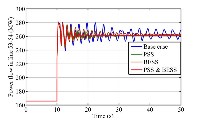
Appl. Sci. 2019, 9, 1109                                                                              2 of 22

function (PDF) of wind-output power using a wind speed vs. power curve, which has discontinuities
and is difficult to use in analytical techniques [5]. Thus, there was a need to develop a simple and
accurate probabilistic model for wind-output power. The effect of PVG considering fluctuations on SSS
was studied in References [8–10]. Unlike wind, solar energy has less variability but higher uncertainty.
Thus, it is also important to analyze its effects on power-system stability. In References [8,9], the effects
of stochastic fluctuations due to PVG on PSSS in a distribution network were studied. The authors
found that PVG has the potential to deteriorate small-signal stability. The impact of PVG using real
measured data on a large transmission system was studied in Reference [10], where the authors
concluded that stochastic fluctuation due to solar irradiance can greatly hamper dynamic stability.
Consequently, there is much need to study the combined effect of the two intermittent renewable
sources on PSSS.
       Power-system stabilizers (PSSs) are generally selected as the first option to improve SSS as they can
be conveniently located at generating stations. However, other power-system devices, such as flexible
AC transmission systems (FACTS), and wind and solar farms incorporating power-oscillation dampers
(PODs), can also enhance low-frequency stability [7,11,12]. In recent times, as a result of its plummeting
cost, research efforts on utilizing battery energy-storage systems (BESSs) to provide different
power-system functions, such as frequency regulation, power-quality improvement, and oscillation
damping have also gained wide popularity [13]. BESS are usually equipped with POD (termed as BESS
controllers in this paper) when they are employed for oscillation damping [14,15]. They can directly
modulate real output power, making them more suitable for oscillation damping compared to PSS and
FACTS devices [14]. As the placement of energy-storage devices is very flexible compared with RES,
it is easier to install them at locations where the controllability index to damp oscillation is highest,
making it a more efficient candidate than RES with POD to improve SSS [16]. There are some recent
studies in the literature that analyze the effect of BESS on low-frequency oscillatory stability [17,18].
The effect of BESS on dynamic stability with high penetration of solar and wind farms was investigated
in Reference [17]. The authors observed that the tuning of a BESS controller is extremely crucial,
and improper tuning may result in oscillatory instability. In Reference [18], the output power of
multiple BESSs was coordinated using particle-swarm optimization (PSO) to enhance dynamic stability.
The method proposed by References [17,18] provides extensive information about the enhancement of
oscillatory stability using a single or multiple BESS(s). However, this approach of only utilizing PSS or
BESS may not be sufficient to enhance low-frequency stability, especially under current large-scale RES
integration. Thus, it is imperative to study more effective solutions, such as the coordination between
PSS and BESS controllers.
       As RES output power varies stochastically, this leads to a change in the operating point of
a power system, creating multiple operating conditions. The controllers developed using deterministic
techniques may not guarantee satisfactory operating performance under these conditions, as they
were developed for single or very few operating points [19,20]. There are few researchers who
have considered controller tuning by directly considering these factors [11,19–22]. Coordination
between WTG incorporating PODs, and PSSs utilizing PSO, was found to be highly successful in
damping low-frequency oscillations under wind uncertainty in Reference [11]. In Reference [19],
PSS parameters were tuned using differential evolution techniques considering generation and load
uncertainties. The tuned PSSs were found to be effective in improving dynamic stability under
multiple operating conditions. In Reference [20], the design of probabilistically robust PSS controllers
with wide-area signals to improve dynamic stability under wind-power fluctuations was proposed.
The so-designed wide-area-based PSSs were found to be effective in improving SSS under different
scenarios. The authors in Reference [21] proposed an optimal tuning method for PSSs and FACTS
controllers that greatly improves PSSS. However, the authors’ technique was based on a Monte Carlo
simulation, which has very high computational time. A modified fruit-fly algorithm was used for
coordinating PSSs and a static-var compensator (SVC) to improve SSS under wind-power fluctuations
in Reference [22]. The proposed strategy is based on a computationally efficient method that optimizes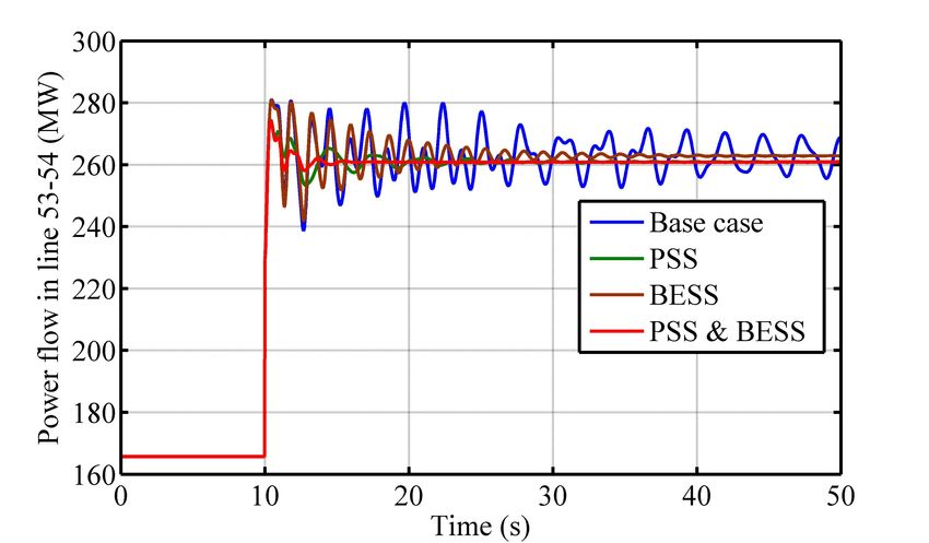
Appl. Sci. 2019, 9, 1109                                                                           3 of 22

the controller parameters in considerably less time. However, all the mentioned studies in the literature
tuned the controllers by considering the same renewable-energy resources [11,20–22] or only load
uncertainty [19]. As can be seen from before the mentioned descriptions, different metaheuristic
techniques were applied to optimally tune power-system controllers considering power-system
uncertainties. We chose a metaheuristic technique known as the firefly algorithm for our study.
The firefly algorithm is a swarm-intelligence method based on flashing patterns and the behavior
of tropical fireflies. It is simple, flexible, easy to implement, and provides better convergence in less
computation time compared to other nature-inspired optimization techniques, such as the genetic
algorithm and PSO [23,24].
     Thus, in this paper, we address the research gaps that exist in the current literature, as described
in the preceding paragraphs. The major contributions of this paper are:

1.    Proposal of a procedure to compute the continuous probability function of RES and use it to
      assess PSSS.
2.    Development of a probabilistic method to optimally tune power-system controllers, such as PSSs
      and BESSs, considering power fluctuation due to RES.
3.    Development of a detailed model of BESSs in DIGSILENT [25], and the study of the effect of
      the proposed control strategy of utilizing BESS controllers and PSS in a coordinated manner on
      probabilistic low-frequency oscillatory stability.
4.    Use of the firefly algorithm to coordinate power-system controllers.

     Thus, the novel contribution of our study is the proposal of a probabilistic method to tune
power-system controllers, such as PSSs and BESSs controllers, considering stochastic power
fluctuation arising due to two popular RES. The proposed method can be divided into two stages:
Stage 1, which computes statistical information about the effect of RES integration on SSS, and Stage
2, which uses this knowledge to coordinate the power-system controllers. As the proposed method
uses a probabilistic method, it is first necessary to model the input uncertainties (RES output power);
however, as stated earlier, and is discussed in detail in subsequent sections, most probabilistic models
of RES either contain discontinuous terms or are incomplete, which makes them difficult to use
in probabilistic analysis. Thus, we also propose a procedure to obtain a probabilistic RES model
that is continuous and can be conveniently applied with probabilistic methods related to the power
system. Lastly, as mentioned in the preceding paragraphs, the modern electric grid continues to
integrate huge amount of RES, and the sole use of PSS and BESS controllers may be insufficient
to improve the SSS margin. Thus, we also propose a strategy to use PSS and BESS controllers in
a coordinated manner and study their effect on PSSS. BESSs, along with controllers, are modeled in
detail in DIGSILENT for this purpose.
     The paper is organized as follows: Section 2 discusses the proposed method to enhance PSSS,
followed by the PSSS assessment method in Section 3. Section 4 describes different power-system
controllers utilized in this paper to enhance dynamic stability, as well as the optimization method to
tune them. The detailed results and discussion under different scenarios are provided in Section 5.
Conclusions drawn are described in Section 6.

2. General Overview of the Proposed Method
     The proposed method to tune power-system controllers considering stochastic power fluctuations
due to RES integration is shown in Figure 1, and is a combination of two main parts: Part 1,
which calculates the statistical SSS information, and Part 2, which utilizes this information to
enhance oscillatory stability by coordinating different power-system controllers, such as PSS and
BESS controllers, with the help of the optimization technique. The overall proposed methodology can
be described as follows: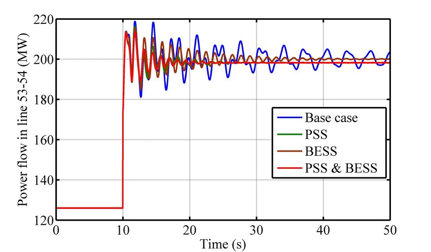
Appl. Sci. 2019, 9, 1109 4 of 22
1. Probabilistic modeling of input random variables (RES output power) using power-forecast error.
The so-obtained probabilistic models are efficient and convenient to use with analytical methods,
and are described in detail in Section 3.1.
2. Input PDFs are then used with an analytical method based on cumulants [2,26] to calculate the
PDF of output random variables. Output random variables in this paper are the real eigenvalue
part (also called the damping constant) and damping factor. The cumulant method was chosen
over other analytical methods, such as point estimate and probabilistic collocation, due to its
higher accuracy as well as computational efficiency [27].
3. Next, the Gram–Charlier expansion method [26] was used with output random variables to
calculate statistical indices that provide information about the small-signal stability margin.
More details for Steps 2 and 3 can be found in Section 3.2.
4. If the system is found to have a critical value of indices with respect to oscillatory stability,
the power-system controllers are then tuned in a coordinated manner. This coordination is
achieved by formulating it as an optimization problem. The objective function of this optimization
problem consists of probabilistic stability indices (obtained from Part 1) and is solved using the
firefly algorithm. The detailed description of this process can be found in Section 4.2.
Moreover, constraints of this optimization problem are the different parameters of power-system
controllers, and solving the optimization problem provides optimized value for the controller
parameters. All controllers, such as PSS and BESS controllers, were modeled in great detail and
can be found in Section 4.1.
Stage1: Analysis Statistical information about SSS Stage2: Optimization
Formulation of objective function
Probabilistic Probabilistic Cumulant
modeling of modeling of Output
method and
power forecast renewable energy Gram-Charlier Solving optimization problem using firefly algorithm
error sources expansion Output
Obtain the optimized parameters for Modeling of PSSs
PSSs and BESS controllers and BESSs
Figure 1. Proposed method to coordinate power-system-stabilizer (PSS) and battery energy-storage-
system (BESS) controllers under renewable-energy-source (RES) integration.
3. PSSS Assessment Using Developed Efficient Probabilistic RES Model
3.1. Development of PVG Probability Function and WTG Output Power
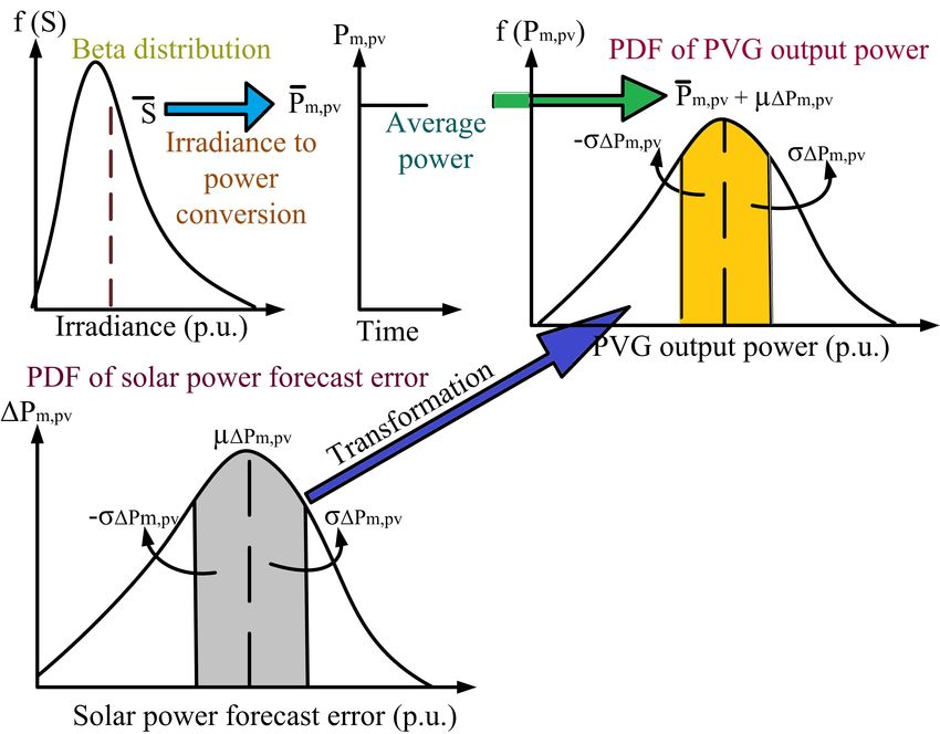
PVG output power increases with solar radiation until it reaches standard solar radiation (around
1000 W/m2 ), beyond which it remains constant at its rated capacity, as shown in Figure 2 [28]. Moreover,
output power from a solar farm is zero at night time. These two situations cause discontinuities in the
PDF of PVG output power when it is computed using the general procedure, and are usually modeled
as impulse functions, as shown in Figure 2 [2,3]. To avoid these discontinuities, researchers [8–10]
commonly only use the linear region (where solar radiation is greater than zero and less than standard
radiation) to compute the PDF of the PVG output power, which results in a continuous function and
is much more convenient to use. However, the realistic probabilistic model of PVG output power
should be a mixed random variable with two impulse functions, and a continuous function between
them. However, this model is difficult to use with analytical methods, and a more efficient method
based on power-forecast error to construct the probability density of PVG output power was utilized
in our study.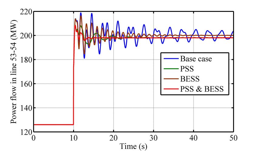
Appl. Sci. 2019, 9, 1109                                                                                                         5 of 22

                     PVG output power (MW)                                 PDF of PVG output power

                Rated power                                                        Impulse function 1       Impulse function 2

                                                                                       Continuous function
                              0                                               0
                                   Solar                         2                   PVG output power (MW) Rated
                                             Solar radiation (W/m )
                                radiation in                                                               power
                           standard environment

      Figure 2.     General procedure for computing the probability density function (PDF) of
      photovoltaic-generation (PVG) power from solar-farm characteristics.

     Both solar-power and wind-power forecast errors are commonly modeled as normal distribution,
and vary with feed-in power as well as the time of day [29,30]. Power-forecast error ∆Pm,pv for an mth
solar farm is defined as
                                       ∆Pm,pv = Pm,pv − P̄m,pv                                     (1)

where Pm,pv is actual output power for solar farm mth , and P̄m,pv is the forecast output power of the
solar farm, which is deterministic (average solar-farm output power [29] in this paper). The probability
function of the power-forecast error can be computed as:

                                                              1                    [∆Pm,pv − µ∆Pm,pv ]2
                                   f (∆Pm,pv ) =                  √        exp −            2
                                                                                                                                    (2)
                                                    σ∆Pm,pv           2π                  2σ∆Pm,pv

where µ∆Pm,pv and σ∆Pm,pv are the mean and standard deviation of solar-power-forecast
error, respectively.
     Thus, the output-power PDF for the mth solar farm can be derived using Equations (1) and (2)
with the help of a transformation:

                                                     1                      [ Pm,pv − ( P̄m,pv + µ∆Pm,pv )]2
                               f ( Pm,pv ) =             √        exp −                    2
                                                                                                                                    (3)
                                               σ∆Pm,pv       2π                          2σ∆Pm,pv

     As wind-power-forecast error is also commonly modeled as normal distribution [5,29,30],
the output-power PDF for the nth wind farm can also be derived in a similar manner to PDF
computation of PVG output power as:

                                                      1                     [ Pn,w − ( P̄n,w + µ∆Pn,w )]2
                                  f ( Pn,w ) =         √          exp −                    2
                                                                                                                                    (4)
                                                 σ∆Pn,w      2π                        2σ∆P  n,w

where P̄n,w , µ∆Pn,w and σ∆Pn,w are the forecast output power of the wind farm, which is deterministic
(average wind-farm output power [29] in this paper), and mean and standard deviation of
wind-power-forecast error respectively.
     Both Equations (3) and (4) are continuous and very convenient to use with analytical methods.
The graphical illustration of PDF computation of PVG output power using solar-power-forecast error
is shown in Figure 3. Beta distribution is commonly used to characterize solar radiation and has some
value of shape parameters a and b depending on location [31]. These shape parameters are then used
to estimate average solar radiation S̄, which is further used to compute the average PVG output power
with the help of solar-farm power characteristics [28] in our work. Finally, the PDF of PVG output
power is obtained by substituting the value of computed average PVG output power into Equation (3).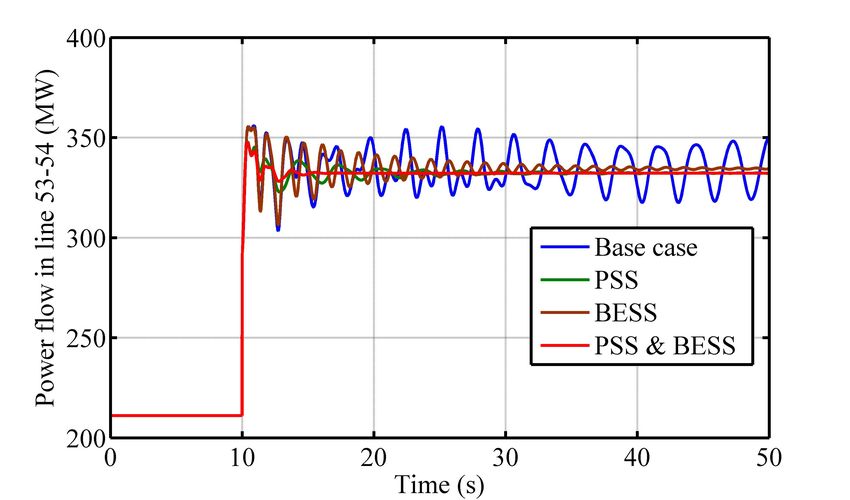
Appl. Sci. 2019, 9, 1109                                                                          6 of 22

The probability-density function of WTG output power can also be obtained in a similar manner, with
the only exception being that Weibull distribution is commonly used to characterize wind velocity [31].

                           Figure 3. Graphical illustration of PDF computation of PVG.

3.2. Stability Index Calculation
     Let λo = αo + jωo denotes the o th eigenvalue of the power system with real part αo and imaginary
part ωo . Damping factor ξ o can be calculated as [32]:

                                                             −αo
                                                ξo = p                                               (5)
                                                            α2o + ωo2

     Damping constant and damping factor are taken as output random variables in this paper, and
their PDFs are calculated using the combined method of cumulant and Gram–Charlier expansion
technique [2,26]. The following stability indices are then defined, which provides information about
the SSS margin [22]:                                Z          αc
                                         P(αo < αc ) =              f αo ( x )dx                     (6)
                                                              −∞

                                        P(αo > αc ) = 1 − P(αo < αc )                                (7)
                                                            Z ξc
                                          P(ξ o < ξ c ) =           f ξ o ( x )dx                    (8)
                                                             −∞

where f αo is the PDF of the damping constant for o th eigenvalue, αc is the critical margin for the
damping constant, ξ c is the critical margin for the damping factor, and f ξ o is the damping-factor PDF
for the o th eigenvalue. Equation (7) provides probabilistic statistical information about SSS. A high
value of this index indicates a low likelihood of a system being small-signal stable and vice versa.
Similarly, Equation (8) provides the damping-factor probability of the o th eigenvalue being less than
the critical damping factor, and a lower value is desirable for this index. Both f αo and f ξ o can be
constructed with the aid of the Gram–Charlier expansion [2,26]. More rigorous details on cumulant
and PSSS theory can be found in References [2–4,8–10,26,29]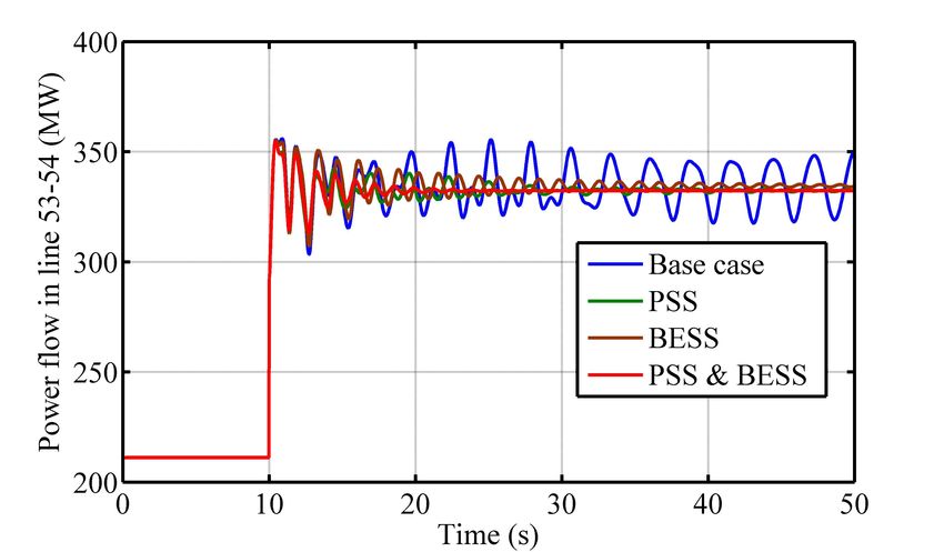
Appl. Sci. 2019, 9, 1109                                                                                             7 of 22

4. Coordination of PSS and BESS Controllers to Enhance Oscillatory Stability Using
Proposed Method
    This section first discusses modeling of controllers that were utilized in our work to enhance
low-frequency oscillatory stability under renewable-resource uncertainties, and the firefly algorithm,
which is used for tuning these controllers.

4.1. Power-System-Controller Modeling

4.1.1. Power-System Stabilizers
      PSS structure is well-established in the literature [6,32], and its primary function is to modulate
excitation-system voltage to improve dynamic stability. A typical PSS connected with a ith generator
with rotor-speed deviation as input constitutes a gain of Ki,pss , lead-lag constant with parameters
T1i,pss , T2i,pss , T3i,pss , T4i,pss , and a washout block with time constant Ti,pssw , as depicted in Figure 4 [6].
The values of maximum voltage Vmax , minimum voltage Vmin , and Ti,pssw are 0.2 and −0.2 p.u. and
10 s, respectively [6]. The range of other PSS parameters is provided in Section 4.2.1.

                                                                                                           Vmax
                                                   STi,pssw            1+ST1i,pss      1+ST3i,pss             Vmod
         Rotor speed            Ki,pss
                                                  1+STi,pssw           1+ST2i,pss      1+ST4i,pss

                               PSS gain           Washout block               Lead-Lag block        Vmin

                                                      Figure 4. ith PSS structure.

4.1.2. Modeling of Sodium–Sulfur-Based BESS and Its Controllers in DIGSILENT
     The schematic diagram depicting the main BESS controllers available in DIGSILENT [25] is shown
in Figure 5. However, the battery model, as well as its controllers in DIGSILENT, are generic and
thus suitably modified to meet our purpose, which is described in detail in the subsequent sections.
Controllers can be divided into three main types: real and reactive power controllers (P-Q controllers),
charge controllers, and power-oscillation damping controllers. We used a sodium–sulfur (NaS) battery
among the many battery technologies in our study as it has high energy density, efficiency, and quick
response time (milliseconds), making it very useful to improve functions related to power-system
stability [33]. The diagram displaying the developed model of NaS-based BESS with controllers in
DIGSILENT is shown in Figure 6.

                                            Pline,i

                                           POD                 Pc
                                         Pmod
                                                          id                           idref
                           P       PQ controller               Charge controller               To converter
                           Q                                                          iqref
                                                          iq
                                                               SOC Vbatt      Ib
                                                               From Battery

                                    Figure 5. Schematic diagram of BESS controllers.
Appl. Sci. 2019, 9, 1109 8 of 22
DIgSILENT
Frame_BatteryCntrl:
P
0
0
PQ-Measurement Q
1 1
StaPqmea
0
Pref 2
PQ Controller
3 ElmDsl*
id
POD_PQ Pline Pmod
1
StaPqmea POD 4
ElmDSL*
5 0
iq
6
idref
0 0
1
Converter
Charge Controller ElmGenstat*
2 1
Vbatt ElmDSL*
iqref
0 1
3
SOC
Battery 1
ElmComp 2
4
Ib
2
Pc
Figure 6. Developed model of NaS-based BESS with controllers in DIGSILENT.
4.1.2.1. Battery Model
Figure 7 shows the equivalent model of a sodium–sulphur (NaS) battery. Battery voltage varies
linearly with depth of discharge (DOD), as well as affects charging and discharging resistance [34].
DOD and state of charge (SOC) can be computed as:
1
Z
DOD = tdt
Qmax (9)
SOC = 1 − DOD
where Qmax is the maximum battery capacity at fully charged/discharged condition ( Ah). Charging
resistance Rch (Ω) is given by [34]:
Rch = c + dDOD2 + eDOD3 + f DOD4 + gDOD5 + hDOD6 + iDOD7 + jDOD8 + kDOD9 + lDOD10 (10)
and discharging resistance Rdis (Ω) can be found as: [34]:
Rdis = c + dDOD2 + eDOD3 + f DOD4 + gDOD5 + hDOD6 + iDOD7 + jDOD8 + kDOD9 (11)
where c, d, e, f , g, h, i, j, k, and l are polynomial coefficients.
Rdis (DOD)
Rlc Ib
Voc (DOD) Rch (DOD) Vbatt
Figure 7. Equivalent model of NaS battery [34].Appl. Sci. 2019, 9, 1109 9 of 22
Open-circuit battery voltage Voc (V ) can be computed as [34]:
Voc = 2.076, DOD ≤ 0.56
(12)
2.076 − 0.00672DOD, DOD > 0.56
Finally, battery output voltage Vbatt (V ) for discharging mode can be calculated as:
Vbatt = Voc − Rdis Ib − Rlc Ib (13)
and for charging mode as:
Vbatt = Voc + Rch Ib + Rlc Ib (14)
where Rlc is life-cycle resistance Ω, and Ib is battery current A.
4.1.2.2. POD Controller for BESS
The POD structure described in References [21,35] was used in our study and has a similar
structure to PSS. However, unlike most PSSs, input feedback signal for POD can be signals from remote
locations, which are often more effective for oscillation damping than local signals [35].
POD structure is very similar to PSS, and is shown in Figure 8. Lead-time constants for
POD at the ith location are T1i,pod , T3i,pod , and lag-time constants are T2i,pod , T4i,pod , the washout-time
constant is Ti,podw , the POD gain is Ki,pod , and maximum and minimum power limits are Pmax and
Pmin , respectively.
Pmax
STi,podw 1+ST1i,pod 1+ST3i,pod
Pline,i e-sTd Ki,pod
1+STi,podw 1+ST2i,pod 1+ST4i,pod
Pmod
Delay POD gain Washout block Lead-Lag block Pmin
Figure 8. ith POD structure.
Unlike most PSSs, POD input feedback signal can be signals from remote locations that are often
more effective for oscillation damping than local signals [35]. It is assumed that phasor-measurement
units (PMU) that provide these remote signals were installed in our test system. However, there exists
finite delay while transmitting the measured signal from PMU to POD control stations, it is commonly
termed as communication delay or latency [36], and is modeled as e−sTd in our work [35]. Value of
latency Td is taken as 100 ms [35].
The feedback remote signal can be any electrical variables, such as real and reactive power flow
in lines, current flow in lines, bus voltages, and angular differences. Among these variables, we chose
real power flow in lines Pline,i as input for PODs, as both reactive power and bus voltage have exciter
and flux-decay components, and angular differences require an additional phase lead of 90 degrees,
making them less suitable for feedback control [37]. The best input (among many real power flow
in lines) for each POD controller is selected using the residue method [15,20,36]. Output from POD
Pmod was chosen to modulate the real power control loop in contrast to the reactive power loop as
BESSs are located at the ends of the transmission line of our test system given in Section 5.1, in which
case, real power modulation is superior to reactive power modulation [38]. The values of Pmax , Pmin ,
and Ti,podw are 0.2 and 40.2 p.u. and 10 s, respectively [6]. The range of other POD parameters used in
this paper is provided in Section 4.2.1.
4.1.2.3. PQ Controller
The PQ controller has two main loops, the active-power loop and reactive-power loop.
The modeling of these loops is based on decoupled control theory, where d-axis current id controls real
power, and the q-axis current iq controls reactive power [8], as shown in Figure 9. The active-powerAppl. Sci. 2019, 9, 1109 10 of 22
control loop has four main input signals: set point active power Pre f , actual BESS output power P,
modulating signal from POD Pmod , and signal from charge controller Pc . The difference between the
sums of Pre f , Pmod and Pc with P is passed through a simple PI controller to synthesize id . Similarly, iq is
synthesized by measuring the difference between setpoint reactive-power Qre f with actual reactive
power Q and passing it to a PI controller. Qre f commonly depends on the requirement for power-factor
regulation, but is assumed to be zero for this paper (unity power factor).
Pmod Pc
Pref PI id Qref PI iq
P Q
Figure 9. PQ controller for BESS.
The current reference signals from the PQ controller are then fed to the charge controller,
which controls battery charging and discharging, and provides reference currents idre f and iqre f ,
which are used to generate pulse-width modulating signals to control VSC switching.
4.2. Power-System-Controller Tuning Using Optimization Technique
4.2.1. Optimization-Problem Formulation
It is generally more convenient to use standardized expectations of damping constant α∗o and
damping factor ξ o∗ for optimization studies, which are given by [22]:
α¯o ∗ ξ¯o
α∗o = , ξo = (15)
σαo σξ o
where α¯o , ξ¯o , σαo , and σξ o are the expected value of the o th damping constant, the expected value of
o th damping factor, standard deviation of the o th damping constant, and standard deviation of the
o th damping factor, respectively, and can be computed using cumulant theory described in detail in
References [2–4,9,10]. The objective function for the optimization problem is formulated as:
p p
minimization F = J1 ∑ P(α∗o > αc ) + J2 ∑ P(ξ o∗ < ξ c ) (16)
i =1 i =1
subject to [6]:
0.1 ≤ Ki,pss , Ki,pod ≤ 50
0.01 ≤ T1i,pss , T3i,pss , T1i,pod , T3i,pod ≤ 1.5 (17)
0.01 ≤ T2i,pss , T4i,pss , T2i,pod , T4i,pod ≤ 0.15
Equation (16) is a minimization problem, where the objective is to minimize the likelihood
of standardized expectation of the damping constant being greater than αc , and the standardized
expectation of the damping factor being less than ξ c . The values of αc and ξ c depend on user
requirements, and were chosen as −0.1 and 0.1, respectively, for this paper [19,22]. Equation (16)
can be computed using Equations (7), (8), and (15). Values for both J1 and J2 were chosen to be 0.5,
which corresponds to providing equal weight to both objective functions. Only the electromechanical
eigenvalues of the total p were considered for the optimization problem [19,22].Appl. Sci. 2019, 9, 1109 11 of 22
4.2.2. Solving Optimization Problem Using Firefly Algorithm
The firefly algorithm is one of the most popular swarm-based optimization algorithms, and its
pseudocode is given below:
Algorithm 1: General pseudocode of firefly algorithm
Computation of value for objective function f ( x ) with t decision variables x = ( x1 , x2 , ....xt ) T
Generate initial random population for n fireflies xi (i = 1, 2, 3, ...., n)
Calculate light intensity Li for xi using f ( xi )
Define light-absorption coefficient γ
While (k < Maximum Generation)
for i = 1 : n, all n fireflies
for j = 1 : n, all n fireflies
if (Li < L j ), Move firefly i towards j; end if
Change attractiveness with distance r using exp−γr
Compute new solutions and update light intensity
end for j
end for i
Rank fireflies and find current global best solution gb
end while
The general flowchart of utilizing the firefly algorithm to tune power0system controllers in our
study is shown in Figure 10 and is briefly described as follows:
1. In the first step, each control parameter xi is assigned an array of random numbers, with the total
number size of fireflies Npop as:
xi =[Ki,pod , Ki,pss , T1i,pod , T1i,pss , T2i,pod , T2i,pss , T3i,pod , T3i,pss , T4i,pod , T4i,pss ] (18)
2. Control parameters are then used to compute the objective function using Equation (16),
whose values represent firefly light intensity. The fireflies are then sorted and accordingly ranked.
The so-obtained control parameters after ranking are termed as x j .
3. The movement of less-bright fireflies xi to brighter fireflies x j is given by:
−γrij2
xit+1 = xit + β exp x tj − xit + αt εtj (19)
where xit+1 is the position of the fireflies at the next iteration, β is the attractiveness coefficient,
εtj is the vector of random numbers, γ is the light-absorption constant, αt is the randomization
parameter, and rij is the Cartesian distance between two fireflies.
4. If the value of a control parameter exceeds its range, it is reset back to its maximum or minimum
value, depending upon its nearness to the extreme value given by Equation (17).
5. Continue to the next iteration until the maximum number of iterations is reached.Appl. Sci. 2019, 9, 1109 12 of 22
Start
Generate a initial population of Npop fireflies for search parameter
[Ki,pss T1i,pss T2i,pss T3i,pss T4i,pss Ki,pod T1i,pod T2i,pod T3i,pod T4i,pod ]
Evaluate light intensity from objective
function (16) and rank the fireflies
Move the fireflies to more brighter
intensities using (19)
Verify that the parameters are within the
range using (17)
Iteration=Iteration +1 Iteration > Max Iteration
No
Yes
Stop
Figure 10. Flowchart of proposed method for optimal tuning of power-system controllers.
5. Results and Discussion
5.1. Test System
The test system is a modified IEEE 68 bus network, which is a benchmark system to study
low-frequency oscillatory dynamics in power systems [39]. This system has fifteen synchronous
generators, three wind farms, and three solar farms, as shown in Figure 11. Deterministic eigenvalue
analysis [32] was first run to determine RES locations. Table 1 shows the damping constant and
damping factor of the three most critical eigenvalues obtained for the test system without any RES.
The major areas associated with the critical eigenvalues are 3, 4, and 5, and a similar conclusion was
also reached in Reference [39]. Thus, we decided to install RES at Areas 3, 4, and 5, which represent the
worst-case scenario with respect to SSS. The countries leading the way in PVG and WTG generally have
a penetration level in the range of 20%–30% [1]. By taking this fact into consideration, we assumed
a 30% RES penetration level in their respective areas, resulting in the size of solar and wind farm at
Areas 3, 4 and 5 being 150, 172, and 370 MVA, respectively.
Table 1. Results of deterministic eigenvalue analysis without RES.
No. Damping Constant Damping Factor Frequency (Hz) Associated Areas
1 −0.0102 0.0450 0.3607 2, 4 and 5
2 −0.0700 0.0164 0.6792 4 and 5
3 −0.0912 0.0183 0.7922 3 and 4Appl. Sci. 2019, 9, 1109 13 of 22
WG 1 PV 1 BESS 1
WG 2 PV 2 BESS 2
WG 3 PV 3 BESS 3
Figure 11. Modified test system with RES.
All generators consist of a fast-acting static excitation system; the details of generators, excitation
systems, and line parameters can be found in Reference [37]. This paper uses a DIGSILENT
built-in wind-farm model that is similar to Type-3 doubly fed induction generators with a rotor-side
converter [25], and the PVG model that is available in DIGSILENT [25]. WTG and PVG parameters
used in this paper are provided in Appendix A. Generator 1 (G1) to Generator 12 (G12) were assumed
to be equipped with PSS. Areas 3 to 5 had large power generation and inertia, so any generator outage
in these areas might seriously jeopardize system frequency [40]. Hence, one BESS is assumed to be
connected in Areas 3, 4, and 5. As BESSs have not yet primarily been connected for small-signal
stability purposes in the current electric-power system, we used the method proposed by the authors
of Reference [41], which can be used to calculate BESS size for frequency regulation; the obtained BESS
size after applying this method was not optimal, but still provides realistic battery size and is better
than using an arbitrary size for analysis. Moreover, we also assumed unity power-factor operation
of BESSs in our study. Thus, the size of BESS located in Areas 3, 4, and 5 was 26, 60, and 75 MVA,
respectively. More details about battery-capacity determination and parameters are provided in
Appendix A.
5.2. Simulation Results
5.2.1. Results under Different Controller Configurations
This section describes the obtained statistical results related to the stability of critical eigenvalues
(also termed as modes) for four different controller configurations: case study with no controllers
(base case), case study with only PSSs, case study with only BESS controllers, and case study with the
proposed strategy of using PSS and BESS controllers.
The base case was run by disconnecting all PSSs and BESSs. The obtained result using the PSSS
assessment method (described in Section 3) was first compared with MCS (10,000 simulations with
95% confidence interval) to verify its accuracy. Figure 12 shows that the PDF of the most critical
eigenvalue (nearest eigenvalue to origin), obtained using the analytical method, very closely resembles
MCS.Furthermore, the average root mean square [26] and computation time of the analytical method
were found to be 0.1731% and 72.6 s, respectively, highlighting the accuracy and computational
efficiency of the analytical method.Appl. Sci. 2019, 9, 1109 14 of 22
Figure 12. Damping constant of most critical eigenvalue.
The probabilistic stability indices obtained for all critical electromechanical modes (15 in total)
under the no-controller case study are shown under the base case heading in Table 2. The probability
of the damping constant being greater than −0.1 was very high for Modes 1 to 4 under the base case.
Furthermore, the damping factor of all modes had a 100% probability of being lower than 10% for the
case without controllers. Both of these values suggest that the given test system under the base case
has much potential to be small-signal unstable. This result led us to investigate potential solutions for
this problem.
Table 2. Comparison of stability indices under different controller conditions using proposed method.
No Controllers PSSs BESS Controllers PSSs and BESS Controllers
No. P (α > −0.1) P (ξ < 0.1) P (α > −0.1) P (ξ < 0.1) P (α > −0.1) P (ξ < 0.1) P (α > −0.1) P (ξ < 0.1)
{%} {%} {%} {%} {%} {%} {%} {%}
1 100 100 0 95.9100 0 0 0 0
2 96.5000 100 90.6403 100 0 0 0 0
3 92.0600 100 95.4195 100 0 0 0 0
4 94.4200 100 0 0 0 100 0 0
5 0 100 0 0 0 100 0 0
. " " " " " " " "
15 0 100 0 0 0 100 0 0
Note in Table 2 and here afterwards in our paper, the symbol (") refers to the ditto mark.
The second controller configuration only considered PSS operation and assumed all BESSs to be
disconnected. The PSSs located at Generators 1 to 12 were then simultaneously tuned using the
proposed method. A population size of 50 fireflies was chosen, as this size is commonly selected by
most swarm-based intelligence algorithms that are used to solve optimization problems related to
low-frequency stability [11,19]. The values of β, αt , and γ were calculated from the average length of
controller parameters and are shown in Table 3. The optimization algorithm was solved using Intel (R)
Core (TM) i5-2400 CPU, 3.1 GHz processing speed, with 8 GB RAM, and it took 3.15 h to compute.
However, as the optimization algorithm provides the stochastic output, 30 repeated evaluations were
performed and the average was used for analysis in this paper [24]. All programs were written using
DIGSILENT programming language [25].
Table 3. Parameters of firefly algorithm.
Npop β αt γ Repeated Evaluations
50 0.4136 0.2 1 30
Table 2, under the PSS category, shows that, except for Modes 2 and 3, there was a low likelihood
that the damping constant of other modes was greater than their margin. From a damping=factor
perspective, Modes 1 to 3 had high probability of being less than the critical damping value,
which shows that only employing PSSs is insufficient to provide required damping under stochastic
PVG and WTG penetration. However, probabilistic statistics related to SSS were much improved inAppl. Sci. 2019, 9, 1109 15 of 22
the case with only-PSS connection compared with the base case. Specifically to improve Modes 1 to
3, we performed further investigations. They were found to be interarea modes that are generally
difficult to improve by only using PSSs. Thus, BESS controllers were sought to improve them, which is
discussed below.
The results under the BESS controller category of Table 2 were computed by assuming all three
BESS controllers of the test system were connected, and all PSSs were disabled. It was first necessary
to find the best feedback signal for each BESS controller before tuning them. This paper uses residue
analysis for this purpose, as discussed in Section 4.1.2.2. The signal that provides the highest residue for
BESS1, BESS2, and BESS3 was found to be an active power flow between Lines 45 to 51, active power
flow between Lines 41 to 42, and real power flow between Lines 43 to 44, respectively. The proposed
method was then used to tune the BESS controllers.
The previously risked Modes 1 to 3 in the case with only PSSs, which have a high likelihood of
being small-signal unstable, have a low likelihood of being low-frequency unstable, as can be seen
from Table 2 for the case with BESS controllers. However, the probability of the damping constant
being greater than the critical margin, and the probability of the damping factor being lower than the
critical margin for other modes (4–15) increases drastically for this controller configuration. This is
largely because they are mainly local modes that cannot be effectively damped by only using BESS
controllers as they use remote signals from the PMU.
The final controller configuration case considers the test system with a connection of both BESS
controllers and generators (1–12) with PSS. The objective function given by Equation (16) is first solved
to obtain the optimized parameters for all PSSs and POD controllers. The convergence of the objective
function is shown in Figure 13, and the minimum value of 5123 was achieved in 44 iterations.
Figure 13. Objective-function convergence.
As can be seen from Table 2 under the PSS and BESS controller heading, all modes have a low
probability of being small-signal unstable with respect to their margin values, showing the effectiveness
of the proposed coordinating approach of utilizing PSS and BESS controllers.
In addition, we used the optimization-based tuning method (OBTM) proposed by Reference [42]
to compare the effectiveness of our proposed method. The probabilistic indices related to small-signal
instability are always lower with the controllers tuned using the proposed method than the compared
method, as can be seen from Table 4.
Table 4. Comparison of stability indices under different controller conditions using the
optimization-based tuning method (OBTM).
No Controllers PSSs BESS Controllers PSSs and BESS Controllers
No. P (α > −0.1) P (ξ < 0.1) P (α > −0.1) P (ξ < 0.1) P (α > −0.1) P (ξ < 0.1) P (α > −0.1) P (ξ < 0.1)
{%} {%} {%} {%} {%} {%} {%} {%}
1 100 100 0 97.9797 0 0 0 0
2 96.5000 100 94.3965 100 0 0 0 0
3 92.0600 100 97.5650 100 0 0 0 0
4 94.4200 100 0 0 0 100 0 0
5 0 100 0 0 0 100 0 2.7340
6 0 100 0 0 0 100 0 2.2390
. " " " " " " " "
15 0 100 0 0 0 100 0 0Appl. Sci. 2019, 9, 1109 16 of 22
5.2.2. Comparison of Different Controller Cases Under Different Scenarios
To further demonstrate the effectiveness of the controllers tuned using the proposed method, we
analyzed it under three critical scenarios, as shown in Table 5.
Table 5. Details of different scenarios.
No. Details Applied disturbance for time-domain simulation
1 Disconnection of critical Line 53–54 Outage of Line 53–54 at 10 s
2 Increase load of the whole system by 4% Outage of Line 53–54 at 10 s
3 Increase generation of the whole system by 4% Outage of Line 53–54 at 10 s
Tables 6–8 describe the results obtained by tuning controllers using the proposed method under
different scenarios. The probabilistic indices describing SSS instability are very low without controllers,
and improve a bit, particularly for Modes 1–3 in the case with connecting only BESS controllers.
Furthermore, except for a few modes (1–3), the likelihood of the system being dynamically stable is
high in the case of the system with only PSSs, and highest in the case of the proposed strategy of
coordinating PSS and BESS controllers for all scenarios.
Table 6. Stability indices under different controller conditions for Scenario 1 using the
proposed method.
No Controllers PSSs BESS Controllers PSSs and BESS Controllers
No. P (α > −0.1) P (ξ < 0.1) P (α > −0.1) P (ξ < 0.1) P (α > −0.1) P (ξ < 0.1) P (α > −0.1) P (ξ < 0.1)
{%} {%} {%} {%} {%} {%} {%} {%}
1 100 100 0 98.9374 0 0 0 0
2 100 100 6.0612 100 0 0 0 0
3 96.4595 100 93.4344 100 0 0 0 0
4 98.9926 100 0 0 0 100 0 0
5 0 100 0 0 0 100 0 0
. " " " " " " " "
15 0 100 0 0 0 100 0 0
Table 7. Stability indices under different controller conditions for Scenario 2 using the
proposed method.
No Controllers PSSs BESS Controllers PSSs and BESS Controllers
No. P (α > −0.1) P (ξ < 0.1) P (α > −0.1) P (ξ < 0.1) P (α > −0.1) P (ξ < 0.1) P (α > −0.1) P (ξ < 0.1)
{%} {%} {%} {%} {%} {%} {%} {%}
1 100 100 93.7333 100 0 0 0 0
2 100 100 98.1607 100 0 0 0 0
3 97.1333 100 0 0 0 0 0 0
4 98.5768 100 0 0 0 100 0 0
5 0 100 0 0 0 100 0 0
. " " " " " " " "
15 0 100 0 0 0 100 0 0
Table 8. Stability indices under different controller conditions for Scenario 3 using the
proposed method.
No Controllers PSSs BESS Controllers PSSs and BESS Controllers
No. P (α > −0.1) P (ξ < 0.1) P (α > −0.1) P (ξ < 0.1) P (α > −0.1) P (ξ < 0.1) P (α > −0.1) P (ξ < 0.1)
{%} {%} {%} {%} {%} {%} {%} {%}
1 100 100 100 100 0 0 0 0
2 96.8426 100 1.0060 100 0 0 0 0
3 95.1850 100 95.5373 100 0 0 0 0
4 98.2310 100 0 0 97.8950 100 0 0
5 0 100 0 0 0 100 0 0
. " " " " " " " "
15 0 100 0 0 0 100 0 0Appl. Sci. 2019, 9, 1109 17 of 22
The statistical results obtained by tuning controllers using the compared method for different
scenarios is given in Tables 9–11, and the system SSS margin is always less when compared with the
proposed method under all scenarios.
Table 9. Stability indices under different controller conditions for Scenario 1 using OBTM.
No Controllers PSSs BESS Controllers PSSs and BESS Controllers
No. P (α > −0.1) P (ξ < 0.1) P (α > −0.1) P (ξ < 0.1) P (α > −0.1) P (ξ < 0.1) P (α > −0.1) P (ξ < 0.1)
{%} {%} {%} {%} {%} {%} {%} {%}
1 100 100 3.2220 97.1100 0 0 0 0
2 100 100 2.0290 100 2.6651 0 0 0
3 96.4595 100 98.3940 100 0 0 0 0
4 98.9926 100 0 0 0 100 1.8995 0
5 0 100 0 0 0 100 0 0
. " " " " " " " "
15 0 100 0 0 0 100 0 0
Table 10. Stability indices under different controller conditions for Scenario 2 using OBTM.
No Controllers PSSs BESS Controllers PSSs and BESS Controllers
No. P (α > −0.1) P (ξ < 0.1) P (α > −0.1) P (ξ < 0.1) P (α > −0.1) P (ξ < 0.1) P (α > −0.1) P (ξ < 0.1)
{%} {%} {%} {%} {%} {%} {%} {%}
1 100 100 99.0866 100 0 0 0 0
2 100 100 99.3710 100 0 0 0 0
3 97.1333 100 0 0 0 0 0 2.8950
4 98.5768 100 0 0 0 100 0 0
5 0 100 0 0 0 100 0 0
. " " " " " " " "
15 0 100 0 0 0 100 0 0
Table 11. Stability indices under different controller conditions for Scenario 3 using OBTM.
No Controllers PSSs BESS Controllers PSSs and BESS Controllers
No. P (α > −0.1) P (ξ < 0.1) P (α > −0.1) P (ξ < 0.1) P (α > −0.1) P (ξ < 0.1) P (α > −0.1) P (ξ < 0.1)
{%} {%} {%} {%} {%} {%} {%} {%}
1 100 100 100 100 0 0 0 0
2 96.8426 100 1.8218 100 0 0 0 0
3 95.1850 100 100 100 0 0 0 0
4 98.2310 100 0 0 0 100 0 0
5 0 100 0 0 0 100 0 0
. " " " " " " " "
15 0 100 0 0 0 100 0 0
To validate the statistical results, time-domain simulations were also run for both the proposed
method and OBTM under different scenarios. Figure 14 shows the power-flow plots through critical
Line 53–54, P53–54 when a circuit is disconnected under different controller configurations (tuned using
both the proposed method and OBTM) for different scenarios. P53–54 oscillates largely without any
controller, and time response improves with the separate application of PSS and BESS controllers.
Furthermore, both oscillation settling time and amplitude are lowest with the proposed strategy of
utilizing PSS and BESS controllers in a coordinated manner when compared with other controller
configurations, thus highlighting the efficiency of the proposed control strategy. Furthermore, it can
also be seen that the time response of P53–54 following a disturbance is much better when the
power-system controllers are tuned using the proposed method than with the compared method.Appl. Sci. 2019, 9, 1109 18 of 22
(a) (b)
(c) (d)
(e) (f)
Figure 14. Time-domain simulations under different scenarios. (a) Responses using the proposed
method under Scenario 1. (b) Responses using OBTM under Scenario 1. (c) Responses using the
proposed method under Scenario 2. (d) Responses using OBTM under Scenario 2. (e) Responses using
the proposed method under Scenario 3. (f) Responses using OBTM under Scenario 3.
Overshoot [43] and settling-time [43] values for both the proposed and compared method for the
time characteristics of P53–54 are given in Tables 12 and 13. The overshoot and settling-time values were
less for all cases when controllers were tuned using the proposed method when compared to OBTM,
highlighting the effectiveness of the developed method. It should be noted that scenarios without any
controllers are unstable; thus, no time characteristics were calculated for them.
Table 12. Comparison of time responses of P53–54 using the proposed method.
No Controllers PSSs BESS Controllers PSSs and BESS Controllers
Scenario
OS (%) Ts (s) OS (%) Ts (s) OS (%) Ts (s) OS (%) Ts (s)
1 - - 5.1581 19.3900 6.8738 26.0372 5.1398 12.9783
2 - - 5.3265 19.8046 8.1256 25.0869 5.2671 13.0508
3 - - 4.7237 19.3348 6.1518 29.9032 4.6581 13.1429
Table 13. Comparison of time responses of P53–54 using OBTM.
No Controllers PSSs BESS Controllers PSSs and BESS Controllers
Scenario
OS (%) Ts (s) OS (%) Ts (s) OS (%) Ts (s) OS (%) Ts (s)
1 - - 7.2815 22.4320 6.9164 32.0292 9.9199 20.8999
2 - - 9.1993 20.8999 7.6818 29.7599 7.5793 18.2493
3 - - 6.7955 27.9364 6.2899 31.2617 6.7386 17.3451Appl. Sci. 2019, 9, 1109 19 of 22
6. Conclusions
In this paper, an analytical method based on a combined cumulant and Gram–Charlier expansion
method was used to analyze SSS under RES penetration. The results show that stochastic power
fluctuation due to wind and solar farms has the potential to deteriorate low-frequency oscillatory
stability. Hence, we proposed a method to optimally tune power-system controllers to improve PSSS
that takes into account output-power variation from RES. The proposed method was first used to tune
PSSs that were found to mostly improve local modes, but be ineffective in improving interarea modes.
Furthermore, the proposed method was applied to tune POD controllers of NaS-based BESSs, and was
found to be effective in mainly damping interarea modes. Finally, the effect of using the proposed
strategy of utilizing both PSS and BESS controllers in a coordinated manner, whose parameters
are tuned using the proposed method, was studied. This proposed strategy was observed to be
highly efficient in enhancing PSSS even under stochastic power fluctuation due to RES integration.
These results were also confirmed with the aid of time-domain simulation responses conducted
under different scenarios. Moreover, the power-system controllers tuned using the proposed method
provided a better small-signal stability margin than the compared method [42].
In future studies, better sizing and optimal BESS location will be done to improve PSSS under
RES integration. The effect of variable latencies on coordinating controllers will also be studied.
Author Contributions: conceptualization, S.G., S.N., and A.S.; methodology, S.G.; software, S.G.; validation, S.G.,
S.N., and A.S.; formal analysis, S.G.; investigation, S.G.; writing—original-draft preparation, S.G.; writing—review
and editing, S.G.; supervision, S.N. and A.S.
Funding: This research received no external funding.
Acknowledgments: The authors would like to express thanks for the Petchra Pra Jom Klao research scholarship,
funded by the King Mongkut’s University of Technology, Thonburi for the support.
Conflicts of Interest: The authors declare no conflict of interest.
Appendix A. PVG, WTG, and BESS Parameters
Appendix A.1. PVG Data
a = 6.38, b = 3.43, Sc = 100 W/m2 , Sstd = 1000 W/m2 , P1,rp = 370 MW, P2,rp = 172 MW,
P3,rp = 150 MW.
Appendix A.2. PVG Power Forecast Error Data
µ∆P1,pv = 0, µ∆P2,pv = 0, µ∆P3,pv = 0, σ∆P1,pv = 0.5862 p.u., σ∆P2,pv = 0.586 p.u., σ∆P3,pv = 0.588 p.u.
Appendix A.3. PVG Controller Parameters
Active-power gain: 0.1 p.u., active-power time constant: 0.05 s, converter time constant: 0.015 s,
reactive-power gain: 0.1 p.u., reactive-power time constant: 0.05 s.
Appendix A.4. Wind-Turbine Data
k = 1.75, c = 8.78, vc = 3 m/s, vr = 13 m/s, v p = 25 m/s, P1,rw = 370 MW, P2,rw = 172 MW,
P3,rw = 150 MW
Appendix A.5. Wind-Power Forecast-Error Data
µ∆P1,w = 0, µ∆P2,w = 0, µ∆P3,w = 0, σ∆P1,w = 0.4354 p.u., σ∆P2,w = 0.4343 p.u., σ∆P3,w = 0.432 p.u.
Appendix A.6. WTG Controller Parameters
Active-power gain: 0.5 p.u., active-power time constant: 0.002 s, reactive-power gain: 0.5 p.u.,
reactive-power time constant: 0.02 s, coupling reactance: 0.1 p.u., gain of reactive current controller:Appl. Sci. 2019, 9, 1109 20 of 22
1 p.u., integrator time constant of reactive current controller: 0.002 s, gain of active current controller:
1 p.u., integrator time constant of active current controller: 0.002 p.u.
Appendix A.7. BESS Size Determination
BESS1: Droop: 0.0036 p.u., nominal frequency: 60 Hz, steady-state frequency: 59.2 Hz, contingency
considered: Line 18–50. BESS2: Droop: 0.0036 p.u., nominal frequency: 60 Hz, steady-state frequency:
59.2 Hz, contingency considered: Line 41–42. BESS3: Droop: 0.0036 p.u., nominal frequency: 60 Hz,
steady-state frequency: 59.2 Hz, contingency considered: Line 40–41.
Appendix A.8. Battery Parameters
BESS1 rating: 75 MVA, 75 MWh, number of cells in parallel: 500, number of cells in series: 100,
cell capacity per cell: 300 Ah, Qmax = 75 MWh. BESS2 rating: 60 MVA, 60 MWh, number of cells in
parallel: 445, number of cells in series: 150, cell capacity per cell: 300 Ah, Qmax = 60 MWh. BESS3 rating:
26 MVA, 26 MWh, number of cells in parallel: 193, number of cells in series: 150, cell capacity per cell:
300 Ah, Qmax = 26 MWh.
All BESSs have the same polynomial coefficients and lifecycle resistance:
c = 1.48 ∗ 101 , d = −3.6 ∗ 1010 , e = 4 ∗ 10−1 , f = −2.41 ∗ 10−2 , g = 8.7 ∗ 10−4 , h = 1.96 ∗ 10−5 ,
i = 2.76 ∗ 10−7 , j = −2.38 ∗ 10−9 , k = 1.14 ∗ 10−11 , l = −2.34 ∗ 10−14 , Rlc = 0.001 Ω.
Appendix A.9. BESS Controller Parameters
Active current controller: 0.1 p.u., integrator time constant of active current controller: 0.05 s,
active current controller: 0.1 p.u., integrator time constant of active current controller: 0.05 s, converter
delay: 0.015 s.
References
1. REN21 Secretariat. Global Status Report; REN21 Secretariat: Paris, France, 2018.
2. Bu, S.; Du, W.; Wang, H.; Chen, Z.; Xiao, L.; Li, H. Probabilistic analysis of small-signal stability of large-scale
power systems as affected by penetration of wind generation. IEEE Trans. Power Syst. 2012, 27, 762–770.
[CrossRef]
3. Bu, S.; Du, W.; Wang, H. Probabilistic analysis of small-signal rotor angle/voltage stability of large-scale
AC/DC power systems as affected by grid-connected offshore wind generation. IEEE Trans. Power Syst.
2013, 28, 3712–3719. [CrossRef]
4. Bu, S.; Du, W.; Wang, H. Investigation on probabilistic small-signal stability of power systems as affected by
offshore wind generation. IEEE Trans. Power Syst. 2015, 30, 2479–2486. [CrossRef]
5. Wang, Z.; Shen, C.; Liu, F. Probabilistic analysis of small signal stability for power systems with high
penetration of wind generation. IEEE Trans. Sustain. Energy 2016, 7, 1182–1193. [CrossRef]
6. Sauer, P.W.; Pai, M. Power System Dynamics and Stability; Prentice Hall: Upper Saddle River, NJ, USA, 1998;
Volume 1.
7. Hannan, M.A.; Islam, N.N.; Mohamed, A.; Lipu, M.S.H.; Ker, P.J.; Rashid, M.M.; Shareef, H. Artificial
Intelligent Based Damping Controller Optimization for the Multi-Machine Power System: A Review.
IEEE Access 2018, 6, 39574–39594. [CrossRef]
8. Liu, S.; Liu, P.X.; Wang, X. Stability analysis of grid-interfacing inverter control in distribution systems
with multiple photovoltaic-based distributed generators. IEEE Trans. Ind. Electron. 2016, 63, 7339–7348.
[CrossRef]
9. Liu, S.; Liu, P.X.; Wang, X. Stochastic small-signal stability analysis of grid-connected photovoltaic systems.
IEEE Trans. Ind. Electron. 2016, 63, 1027–1038. [CrossRef]
10. Gurung, S.; Naetiladdanon, S.; Sangswang, A. Impact of photovoltaic penetration on small signal stability
considering uncertainties. In Proceedings of the 2017 IEEE Innovative Smart Grid Technologies-Asia
(ISGT-Asia), Auckland, New Zealand, 4–7 December 2017; pp. 1–6.Appl. Sci. 2019, 9, 1109 21 of 22
11. Huang, H.; Chung, C. Coordinated damping control design for DFIG-based wind generation considering
power output variation. IEEE Trans. Power Syst. 2012, 27, 1916–1925. [CrossRef]
12. Shah, R.; Mithulananthan, N.; Lee, K.Y. Large-scale PV plant with a robust controller considering power
oscillation damping. IEEE Trans. Energy Convers. 2013, 28, 106–116. [CrossRef]
13. Aneke, M.; Wang, M. Energy storage technologies and real life applications—A state of the art review.
Appl. Energy 2016, 179, 350–377. [CrossRef]
14. Shi, L.; Lee, K.Y.; Wu, F. Robust ESS-based stabilizer design for damping inter-area oscillations in
multimachine power systems. IEEE Trans. Power Syst. 2016, 31, 1395–1406. [CrossRef]
15. Sui, X.; Tang, Y.; He, H.; Wen, J. Energy-storage-based low-frequency oscillation damping control
using particle swarm optimization and heuristic dynamic programming. IEEE Trans. Power Syst. 2014,
29, 2539–2548. [CrossRef]
16. Silva-Saravia, H.; Pulgar-Painemal, H.; Mauricio, J.M. Flywheel energy storage model, control and location
for improving stability: The Chilean case. IEEE Trans. Power Syst. 2017, 32, 3111–3119. [CrossRef]
17. Setiadi, H.; Krismanto, A.U.; Mithulananthan, N.; Hossain, M. Modal interaction of power systems with
high penetration of renewable energy and BES systems. Int. J. Electr. Power Energy Syst. 2018, 97, 385–395.
[CrossRef]
18. Zhu, Y.; Liu, C.; Sun, K.; Shi, D.; Wang, Z. Optimization of Battery Energy Storage to Improve Power System
Oscillation Damping. IEEE Trans. Sustain. Energy 2018. [CrossRef]
19. Wang, Z.; Chung, C.; Wong, K.; Tse, C. Robust power system stabiliser design under multi-operating
conditions using differential evolution. IET Gener. Transm. Distrib. 2008, 2, 690–700. [CrossRef]
20. Ke, D.; Chung, C. Design of probabilistically-robust wide-area power system stabilizers to suppress inter-area
oscillations of wind integrated power systems. IEEE Trans. Power Syst. 2016, 31, 4297–4309. [CrossRef]
21. Rueda, J.L.; Cepeda, J.C.; Erlich, I. Probabilistic approach for optimal placement and tuning of power system
supplementary damping controllers. IET Gener. Transm. Distrib. 2014, 8, 1831–1842. [CrossRef]
22. Bian, X.; Geng, Y.; Lo, K.L.; Fu, Y.; Zhou, Q. Coordination of PSSs and SVC damping controller to improve
probabilistic small-signal stability of power system with wind farm integration. IEEE Trans. Power Syst.
2016, 31, 2371–2382. [CrossRef]
23. Slowik, A.; Kwasnicka, H. Nature Inspired Methods and Their Industry Applications—Swarm Intelligence
Algorithms. IEEE Trans. Ind. Inform. 2018, 14, 1004–1015. [CrossRef]
24. Yang, X.S. Cuckoo search and firefly algorithm: Overview and analysis. In Cuckoo Search and Firefly Algorithm;
Springer: New York, NY, USA, 2014; pp. 1–26.
25. PowerFactory, D. 15, User Manual; DIGSILENT GmbH: Gomaringen, Germany, 2016.
26. Zhang, P.; Lee, S.T. Probabilistic load flow computation using the method of combined cumulants and
Gram-Charlier expansion. IEEE Trans. Power Syst. 2004, 19, 676–682. [CrossRef]
27. Preece, R.; Huang, K.; Milanović, J.V. Probabilistic small-disturbance stability assessment of uncertain power
systems using efficient estimation methods. IEEE Trans. Power Syst. 2014, 29, 2509–2517. [CrossRef]
28. Zulkifli, N.; Razali, N.; Marsadek, M.; Ramasamy, A. Probabilistic analysis of solar photovoltaic output based
on historical data. In Proceedings of the 2014 IEEE 8th International Power Engineering and Optimization
Conference (PEOCO), Langkawi, Malaysia, 24–25 March 2014; pp. 133–137.
29. Ran, X.; Miao, S. Three-phase probabilistic load flow for power system with correlated wind, photovoltaic
and load. IET Gener. Transm. Distrib. 2016, 10, 3093–3101. [CrossRef]
30. Breuer, C.; Engelhardt, C.; Moser, A. Expectation-based reserve capacity dimensioning in power systems
with an increasing intermittent feed-in. In Proceedings of the 2013 10th International Conference on the
European Energy Market (EEM), Stockholm, Sweden, 27–31 May 2013, pp. 1–7.
31. Soroudi, A.; Aien, M.; Ehsan, M. A probabilistic modeling of photo voltaic modules and wind power
generation impact on distribution networks. IEEE Syst. J. 2012, 6, 254–259. [CrossRef]
32. Kundur, P.; Balu, N.J.; Lauby, M.G. Power System Stability and Control; McGraw-Hill: New York, NY, USA,
1994; Volume 7.
33. Castillo, A.; Gayme, D.F. Grid-scale energy storage applications in renewable energy integration: A survey.
Energy Convers. Manag. 2014, 87, 885–894. [CrossRef]
34. Rodrigues, E.; Osório, G.; Godina, R.; Bizuayehu, A.; Lujano-Rojas, J.; Matias, J.; Catalão, J. Modelling and
sizing of NaS (sodium sulfur) battery energy storage system for extending wind power performance in Crete
Island. Energy 2015, 90, 1606–1617. [CrossRef]You can also read