Towards Lifespan Automation for Caenorhabditis elegans Based on Deep Learning: Analysing Convolutional and Recurrent Neural Networks for Dead or ...
←
→
Page content transcription
If your browser does not render page correctly, please read the page content below
sensors
Article
Towards Lifespan Automation for Caenorhabditis elegans Based
on Deep Learning: Analysing Convolutional and Recurrent
Neural Networks for Dead or Live Classification
Antonio García Garví , Joan Carles Puchalt                        , Pablo E. Layana Castro           , Francisco Navarro Moya and
Antonio-José Sánchez-Salmerón *

                                          Instituto de Automática e Informática Industrial, Universitat Politècnica de València, 46022 Valencia, Spain;
                                          angar25a@upv.edu.es (A.G.G.); juapucro@doctor.upv.es (J.C.P.); pablacas@doctor.upv.es (P.E.L.C.);
                                          franamo4@etsii.upv.es (F.N.M.)
                                          * Correspondence: asanchez@isa.upv.es

                                          Abstract: The automation of lifespan assays with C. elegans in standard Petri dishes is a challenging
                                          problem because there are several problems hindering detection such as occlusions at the plate edges,
                                          dirt accumulation, and worm aggregations. Moreover, determining whether a worm is alive or dead
                                          can be complex as they barely move during the last few days of their lives. This paper proposes
                                          a method combining traditional computer vision techniques with a live/dead C. elegans classifier
                                          based on convolutional and recurrent neural networks from low-resolution image sequences. In
                                          addition to proposing a new method to automate lifespan, the use of data augmentation techniques

                                   is proposed to train the network in the absence of large numbers of samples. The proposed method
Citation: García Garví, A.; Puchalt,
                                          achieved small error rates (3.54% ± 1.30% per plate) with respect to the manual curve, demonstrating
J.C.; Layana Castro, P.E.; Navarro        its feasibility.
Moya, F.; Sánchez-Salmerón, A.-J.
Towards Lifespan Automation for           Keywords: C. elegans; lifespan automation; deep learning; computer vision
Caenorhabditis elegans Based on Deep
Learning: Analysing Convolutional
and Recurrent Neural Networks for
Dead or Live Classification. Sensors      1. Introduction
2021, 21, 4943. https://doi.org/
                                                In recent decades, the nematode Caenorhabditis elegans (C. elegans) has emerged as
10.3390/s21144943
                                          a biological model for the study of neurodegenerative diseases and ageing. Their size
                                          (approximately 1 mm in length) enables their cultivation and handling in standard Petri
Academic Editor: Cosimo Distante
                                          dishes in a cost-effective way, and their transparent body makes it possible to observe their
                                          organs and tissues under a microscope. The complete sequence of the C. elegans genome,
Received: 3 June 2021
Accepted: 19 July 2021
                                          which is similar to that of humans, has been known since 1998 [1]; moreover, its short
Published: 20 July 2021
                                          lifespan (2 to 3 weeks) allows trials to be run in a short time period.
                                                All these characteristics make this nematode an ideal model for the study of ageing.
Publisher’s Note: MDPI stays neutral
                                          Among the assays performed with C. elegans to study ageing, one of the most outstanding
with regard to jurisdictional claims in
                                          is the lifespan assay [2], which consists of counting live nematodes on test plates periodi-
published maps and institutional affil-   cally [3]. The experiment starts from the beginning of adulthood and ends when the last
iations.                                  nematode dies. Using this count, survival curves are created, representing the survival
                                          percentage of the population each day. In this way, the different factors affecting life
                                          expectancy can be compared and contrasted.
                                                In general, survival is determined by whether movement is observed (alive) or not
Copyright: © 2021 by the authors.
                                          (dead). However, in the last days of the experiment, C. elegans become stationary and only
Licensee MDPI, Basel, Switzerland.
                                          make small head or tail movements. Therefore, it is necessary to touch the body of the
This article is an open access article
                                          nematode with a platinum wire to check whether there is a response.
distributed under the terms and                 Today, in many laboratories, time-consuming and laborious handling and monitoring
conditions of the Creative Commons        tasks are performed manually. Automation is, therefore, an attractive proposition, saving
Attribution (CC BY) license (https://     time, providing constant monitoring, and obtaining more accurate measurements.
creativecommons.org/licenses/by/                Automatic monitoring of C. elegans cultured in standard Petri dishes is a complex task
4.0/).                                    due to (1) the great variety of forms or poses these nematodes can adopt, (2) the problem of

Sensors 2021, 21, 4943. https://doi.org/10.3390/s21144943                                                       https://www.mdpi.com/journal/sensors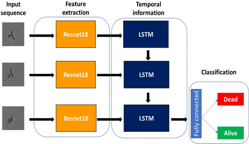
Sensors 2021, 21, 4943                                                                                           2 of 17

                         dirt and condensation on the plate, which requires the use of special methods, and (3) the
                         problem of aggregation of several C. elegans, which requires specific detection techniques.
                               Furthermore, discriminating between dead and live worms presents difficulties as
                         they hardly move in the last few days of their lives, requiring greater precision, longer
                         monitoring times to confirm death and, therefore, higher computational and memory costs.
                               In the literature [4], major contributions can be found that have proposed solutions
                         to the problem of automating lifespan experiments with C. elegans. Some outstanding
                         examples are given below. WormScan [5] was one of the first works to use scanners to
                         monitor C. elegans experiments and determine whether a nematode is alive or dead on
                         the basis of its movement; Lifespan Machine [6] also monitors petri dishes with scanners
                         but with improved optics and systems to control the heat generated by the scanners. In
                         addition, the authors developed their own software to determine whether nematodes
                         are alive or dead. To classify dead worms, they identified stationary worms and track
                         small posture changes to determine the time of death. WorMotel [7] uses specific plates
                         with multiple microfabricated wells, thus allowing individual nematodes to be analysed
                         and avoiding the problem of aggregation. Automated Wormscan [8] takes the WormScan
                         method and makes it fully automatic. WormBot [9] is a robotic system that allows semi-
                         automatic lifespan analysis. Lastly, a method based on vibration to stimulate C. elegans in
                         Petri plates, to confirm whether worms are dead or alive, was proposed in [10].
                               These methods use traditional computer vision techniques that require feature design
                         and manual adjustment of numerous parameters. In recent years, the rise of deep learning
                         has led to breakthroughs in computer vision tasks such as object detection, classification,
                         and segmentation [11–13]. There has been a shift from a feature design paradigm to one of
                         automatic feature extraction.
                               To date, no studies have reported automated lifespan assays with C. elegans using
                         artificial neural networks. However, there has been an increase in the number of stud-
                         ies using machine learning and deep learning to solve other problems related to these
                         nematodes. For example, a C. elegans trajectory generator using a long short-term mem-
                         ory (LSTM) was proposed in [14]. WorMachine [15] is a tool that uses machine learning
                         techniques for the identification, sex classification, and extraction of different phenotypes
                         of C. elegans. A support vector machine (SVM) was used for the automatic detection of
                         C. elegans via a smartphone app in [16]. A method that classifies different strains of C.
                         elegans using convolutional neural networks (CNN) was presented in [17]. Methods based
                         on neural networks have also been proposed for head and tail localisation [18] and pose
                         estimation [19–21]. Recently, [22,23] used different convolutional neural network models to
                         estimate the physiological age of C. elegans. A method for the identification and detection
                         of C. elegans based on Faster R-CNN was proposed in [24]. Lastly, [25] developed a CNN
                         that classifies young adult worms into short-lived and long-lived. They also used this CNN
                         to classify worm movement.
                               This article proposes a method using simple computer vision techniques and neural
                         networks to automate lifespan assays. Specifically, it is a classifier that determines whether
                         a C. elegans is alive or dead by analysing a sequence of images. The architecture combines
                         a pretrained convolutional neural network (Resnet18) with a recurrent LSTM network.
                         In addition to proposing a method to automate lifespan, the use of data augmentation
                         techniques (mainly based on a simulator) has been proposed to train the network despite
                         the lack of a large number of samples. Our method obtained 91% accuracy in classifying C.
                         elegans image sequences as alive or dead from our validation dataset.
                               After training and validating the classifier, this method was tested by automatically
                         counting C. elegans on several real lifespan plates, slightly improving the results of an
                         automatic method based purely on traditional computer vision techniques.
                               The article is structured as follows: the proposed method is presented in Section 2, the
                         experiments are reported in Section 3, and the results are discussed in Section 4.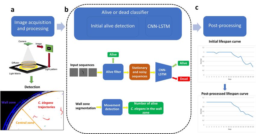
Sensors 2021, 21, 4943                                                                                             3 of 17

                         2. Materials and Methods
                         2.1. C. elegans Strains and Culture Conditions (Lifespan Assay Protocol)
                              The Caenorhabditis Genetics Centre at the University of Minnesota provided the C.
                         elegans of the strains N2, Bristol (wild-type), and CB1370, daf-2 (e1370) that were used to
                         perform the lifespan assays.
                              All worms were age-synchronised and pipetted onto Nematode Growth Medium
                         (NGM) in 55 mm Petri plates. Temperature was maintained at 20 ◦ C. In order to reduce the
                         probability of reproduction, FUdR (0.2 mM) was added to the plates.
                              Fungizone was added to reduce fungal contamination [26]. As a standard diet, strain
                         OP50 of Escherichia coli was used, which was seeded in the middle of the plate as worms
                         tend to stay on the lawn, thus avoiding occluded wall zones.
                              The procedure followed by the laboratory operator on every day of the assay was as
                         follows: (1) He removed the plates from the incubator and placed them in the acquisition
                         system; (2) before starting the capture, he made sure that there was no condensation on the
                         lid and removed it if detected; (3) he captured a sequence of 30 images per plate at 1 fps
                         and returned the plates to the incubator. This reduced the time that the plates were out of
                         the incubator prevented condensation on the lid. In addition, the room temperature was
                         maintained at 20 ◦ C to prevent condensation.

                         2.2. Automated Lifespan Algorithm Based on Traditional Computer Vision Techniques
                              To develop the new method proposed in this article, we took as a starting point the
                         automatic lifespan method based on traditional computer vision techniques proposed
                         in [27]. Parts of this method were taken, such as segmentation, motion detection in the
                         edge zone of the plate, and postprocessing. In addition, this method was used as a baseline
                         to compare the accuracy of the new method in obtaining the lifespan curves.

                         2.3. Proposed Automatic Lifespan Method
                               The problem of counting the number of live C. elegans within a plate, applying deep
                         learning directly from plate image sequences, is a very interesting regression problem.
                         However, neural networks require a dataset with a lot of data to feed the learning process
                         of its millions of parameters. Considering the high cost of obtaining a labelled dataset from
                         these image sequences, traditional computer vision techniques are proposed to simplify
                         the problem to be solved by the neural network to a classification problem.
                               The proposed method solves the problem of classifying whether a C. elegans is alive or
                         dead from a sequence of C. elegans images. This approach requires processing the image
                         sequences from the plate, using traditional computer vision techniques to extract the image
                         sequence of each C. elegans, which is the input to the classifier. Moreover, a cascade classifier
                         is proposed. Initially, trivial cases of live C. elegans are detected using traditional motion
                         detection techniques, leaving the solution of the classification problem where live C. elegans
                         sequences look more similar to dead sequences as a final step for the neural network.
                               Figure 1 shows the stages of the proposed lifespan automation method. Firstly
                         (Figure 1a), the image sequence is captured using the intelligent light system proposed
                         in [28]. Secondly, the image sequences are processed to obtain the images for the classifier
                         input. Then, the classifier (Figure 1b), which consists of two stages (initial detection of live
                         C. elegans and alive/dead classification using a neural network) obtains the number of live
                         and dead C. elegans. Then, a post-processing filter is applied to this result as described
                         in [27], in order to correct the counting errors that may occur due to different factors
                         (occlusions, segmentation errors due to the presence of opaque particles in the medium or
                         the plate lid, decomposition) and, thus, finally obtain the lifespan curve (Figure 1c).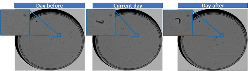
Sensors 2021, 21, 4943
2021, 21, 4943 4 of 17 4 of 17
Figureoverview
Figure 1. General 1. Generalofoverview of themethod:
the proposed proposed
(a)method:
capture (a)
andcapture and processing;
processing; (b) classification;
(b) classification; (c) obtaining lifespan
(c) obtaining
curve and postprocessing.lifespan curve and postprocessing.
2.4. Image
2.4. Image Acquisition Acquisition Method
Method
Images were
Images were captured usingcaptured using the
the monitoring monitoring
system system
developed developed
in [29]. in [29]. This system
This system
uses the active backlight illumination method proposed
uses the active backlight illumination method proposed in [28], which consists of placing in [28], which consists of plac-
an RGB Raspberry Pi camera v1.3 (OmniVision OV5647, which has a resolution ofa resolution of
ing an RGB Raspberry Pi camera v1.3 (OmniVision OV5647, which has
2592a×
2592 × 1944 pixels, 1944size
pixel pixels, a pixel
of 1.4 × 1.4 μm, 1.4 ×field
size aofview 1.4 µm, a view
of 53.50° 53.50◦ size
field ofoptical
× 41.41°, × 41.41 ◦
of , optical size
00 00
1/4′′, and focalofratio
1/4 of , and
2.9)focal ratioofofthe
in front 2.9)lighting
in front system
of the lighting system (a Pi
(a 7′′ Raspberry 7 display
Raspberry Pi display
800 × 480 at
800 × 480 at a resolution at 60
a resolution
fps, 24 bit atRGB60 fps, 24 bit
colour) andRGB
thecolour) andplate
inspected the inspected
in between.plate in between.
A Raspberry Pi 3 was used as a processor to control lighting. The distance between the between the
A Raspberry Pi 3 was used as a processor to control lighting. The distance
camera and thecamera and the
Petri plate wasPetri plate was
sufficient sufficient
to enable to enable
a complete a complete
picture picture
of the Petri of the Petri plate,
plate,
and the camera lens was focused at
and the camera lens was focused at this distance (about 77 mm).this distance (about 77 mm).
With this image With this image
capture capture and
and resolution resolution
setting (1944 ×setting (1944 ×the
1944 pixels), 1944 pixels),
worm sizethe worm size
projects approximately
projects approximately 55 × 3 pixels.
55 × 3 pixels. Although workingAlthough
underworking under these
these resolution resolution conditions
conditions
makes the problem more difficult, it has advantages in
makes the problem more difficult, it has advantages in terms of computational time and terms of computational time and
memory. memory.
2.5. Processing
2.5. Processing
The images captured by the system used have two clearly differentiated zones; on
The images captured by the system used have two clearly differentiated zones; on
the one hand, there is the central zone, which has homogeneous illumination, and, on the
the one hand, there is the central zone, which has homogeneous illumination, and, on the
other hand, there is the wall zone, which has dark areas and noisy pixels. For this reason,
other hand, there is the wall zone, which has dark areas and noisy pixels. For this reason,
these areas are processed independently using the techniques described in [27].
these areas are processed independently using the techniques described in [27].
The central zone (white circle delimited by the orange circumference in Figure 2) was
The central zone (white circle delimited by the orange circumference in Figure 2) was
processed at the worm tracking level (segmentation in red, Figure 2), finally obtaining the
processed at the worm tracking
centroids of the C.level (segmentation
elegans in the last ofinthe
red,
30Figure
images2),making
finally up
obtaining thesequence.
the daily
centroids of the C. elegans in the last of the 30 images making up the daily sequence.
In the wall zone, this tracking is impossible due to the presence of dark areas; however,
In the wallthe
zone, this tracking
capture is impossible
system generates due to the presence
well-illuminated of dark
white rings areas;
that how-
allow the characteristic
ever, the capture system generates well-illuminated white
movements of C. elegans to be partially detected. rings that allow the character-
istic movements of OurC. elegans to be partially
alive/dead criteriondetected.
considers a worm to be dead when it remains in the same
position and posture for more than 1 day. One way to analyse whether a nematode is alive
is to compare the image of the current day with the image of the day before and the day
after. Thus, by simply analysing a sequence of three images, it is possible to determine
whether the worm is alive or dead.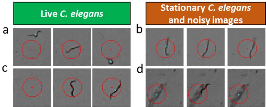
s 2021, 21, 4943 5 of 17
Sensors 2021, 21, 4943 5 of 17
2021, 21, 4943 5 of 17
Figure 2. Result of the processing of the captured sequence. The orange circle delimits the central
zone and the wall zone. In red are the trajectories of C. elegans.
Our alive/dead criterion considers a worm to be dead when it remains in the same
position and posture for more than 1 day. One way to analyse whether a nematode is alive
is toofcompare
Figure
Figure 2. Result 2.
theResult
the
processing
image
of the of the of
ofprocessing
the captured
current
the day The
captured
sequence.
with the image
sequence. of the day
The orange
orange circle delimitscircle
before
delimits
the central
and
thethe
zone
day
central
and the wall zone.
zone and
after. the wall
Thus, by zone. In analysing
simply red are the atrajectories
sequence ofof
C.three
elegans.
images, it is possible to determine
In red are the trajectories of C. elegans.
whether the worm is alive or dead.
Our alive/dead
To generate Tocriterion
the image
generate considers
sequence inaorder
the image worm totodetermine
sequence be
in dead
order when
whetherit remains
the worm
to determine in is
whetherthealive
same
the or
worm is alive or
position and posture
dead, three square for more
dead,sub-images
three square than 1 day.
centred One way
on thecentred
sub-images to
centroid analyse
onofthe whether
thecentroid
current of a nematode
day’s is
C. elegans
the current alive
wereC. elegans were
day’s
iscropped
to comparefromthe
theimage
croppedcurrent of day’s
from the
thecurrent
image,day
current as with
well
day’s thefrom
as
image, image
asthe of thefrom
day and
previous
well as before
the and the
following
previous day
days’
and following days’
after.
images,Thus, byimages,
as shownsimply analysing
in Figure
as shown3. ina Figure
sequence
3. of three images, it is possible to determine
whether the worm is alive or dead.
To generate the image sequence in order to determine whether the worm is alive or
dead, three square sub-images centred on the centroid of the current day’s C. elegans were
cropped from the current day’s image, as well as from the previous and following days’
images, as shown in Figure 3.
Figure 3. Generation of an input sequence.
Figure 3. Generation of an input sequence.
The size of the sub-images was chosen taking into account that the maximum length
of a C. elegans is approximately 55 pixels. In addition, the small displacements and rotations
of the plate that occur when lab technicians place it in the acquisition system each day were
Figure 3. Generation of an input sequence.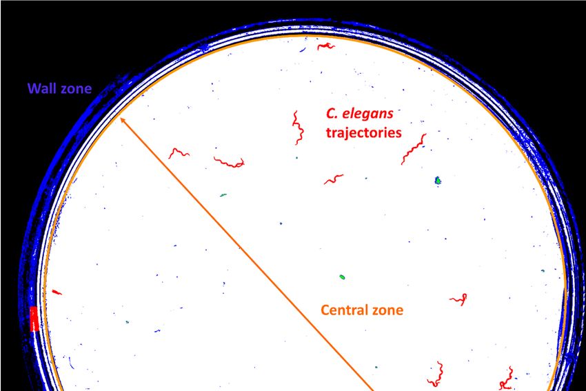
Sensors 2021, 21, 4943                                                                                          6 of 17

                         also taken into account. These displacements are limited because the capture device has
                         a system for fixing the plates. Measurements were taken experimentally to estimate the
                         possible small displacements, obtaining a maximum displacement of 15 pixels.
                              The problem of plate displacements can be addressed using traditional techniques;
                         however, achieving an alignment that works for all sequences is complicated due to
                         potential variability of noise, illumination changes, and aggregation. For this reason, we
                         decided not to perform alignments, but to increase the sub-image size to ensure that it
                         appears completely within the three sub-images if the C. elegans is stationary.
                              Therefore, taking into account the maximum worm length, the maximum estimated
                         displacement of the plate, and a safety margin of 10 pixels, the final size of the sub-images
                         was 80 × 80 pixels, as shown in Figure 3.

                         2.6. Classification Method
                              From these input sequences, various approaches using traditional computer vision
                         techniques can be considered to determine whether a C. elegans is alive or dead. These
                         traditional methods require image alignment and feature design to identify the worm in
                         cases of aggregation or fusion with opaque particles (for example, dust spots on lids) that
                         cause segmentation errors. In addition, C. elegans perform small head or tail movements in
                         the last few days, which are difficult to detect.
                              Our approach was based on using a two-stage cascade classifier. The aim of this
                         cascade processing was to first classify the sequences that are clearly from live C. elegans
                         and let the network decide which cases cannot be determined by the simple motion
                         detection rules.
                              In the first stage, information from the wall zone was processed, and live C. elegans
                         in this zone were estimated using simple motion detection methods. Conversely, in the
                         central zone, sequences of live worms in which C. elegans did not appear in any of the
                         images or moved substantially were detected using simple rules.
                              The remaining more complex cases (stationary C. elegans or with little displacement;
                         images with noise (opaque particles causing segmentation errors)), which would require
                         more advanced techniques and were difficult to adjust, went on to the second stage, which
                         used a neural network to classify these cases as alive or dead.

                         2.7. Initial Detection of Live Worms
                               At this stage, the inputs of the different plate areas (centre and wall) were processed
                         separately.
                               The wall zone was processed using the motion detection algorithm described in [27].
                         The irregular lighting conditions in this area made it necessary to apply movement detection
                         techniques based on temporal analysis of changes in the segmented images. A movement
                         was considered to correspond to C. elegans if the intensity changes of the pixels occurred
                         with low frequency and exceeded an area threshold.
                               For the central zone, the initial detection algorithm analysed each sequence and, in
                         each of the frames, found all the blobs that met a chosen minimum area, taking into account
                         the minimum area that a C. elegans can have (area 20 pixels).
                               In the images for the current day, C. elegans was always found centred in the sub-image
                         (except when there were segmentation errors); thus, it was easy to identify the blob and
                         obtain its centroid. In the remaining frames, the system detected the blobs whose centroid
                         was at a distance from the centroid of the blob of the central frame (current day) of less
                         than a threshold of 20 pixels. This threshold was chosen taking into account the plate
                         displacements (estimated at 15 pixels and with a safety margin of 5).
                               After obtaining the centroids of the blobs (if any) fulfilling the distance constraint,
                         a first classification (live sequences or sequences to be processed by the neural network)
                         was performed, taking into account the following logic: (1) if, in frame 1 (previous day)
                         or in frame 3 (later day), no blob was found meeting the minimum area and distance
                         to the centre constraints, it signified that the C. elegans moved more than the maximum
2021, 21, 4943 7 of 17
Sensors 2021, 21, 4943 7 of 17
was performed, taking into account the following logic: (1) if, in frame 1 (previous day) or
in frame 3 (later day), no blob was found meeting the minimum area and distance to the
centre constraints, it signified that the C. elegans moved more than the maximum distance
(Figure 4a) or distance
was not (Figure
in the image
4a) or(Figure
was not4c) and,image
in the therefore, it could
(Figure be therefore,
4c) and, assured that it be assured
it could
corresponded that
to a itlive worm; (2) otherwise, it may not have moved in any of the three
corresponded to a live worm; (2) otherwise, it may not have moved in any of the
images or it may have
three made
images orsmall
it maydisplacements (Figure
have made small 4b) or it may
displacements have fused
(Figure 4b) or with
it may have fused
noise, producing
witha noise,
segmentation
producing error (Figure 4d) causing
a segmentation non-C.4d)
error (Figure elegans blobs
causing to beelegans
non-C. de- blobs to be
tected. detected.
Figure 4.ofExamples
Figure 4. Examples of imagethat
image sequences sequences that can be
can be classified classified
with withdetection
the initial the initialmethod
detection method
(a,c) and of (a,c)
the stationary
and of the stationary (b) and noisy (d) images classified by the neural network. The red circle is
(b) and noisy (d) images classified by the neural network. The red circle is centred on the centroid of the C. elegans/blob of
centred on the centroid of the C. elegans/blob of the central frame and has a radius of 20 pixels. The
the central frame and has a radius of 20 pixels. The blue dot is the centroid of the blobs detected in the remaining frames.
blue dot is the centroid of the blobs detected in the remaining frames.
With this simple processing method, the first stage classified the live C. elegans in
With this the
simple
wallprocessing
zone and the method,
live C.the first stage
elegans in theclassified the live
central zone, beingC. easily
elegansdetectable
in the following
wall zone and simple
the liverules.
C. elegans
The remaining stationary C. elegans and images with noise,sim-
in the central zone, being easily detectable following which were more
ple rules. The complex
remaining to stationary
classify using C. elegans and images
traditional withwent
techniques, noise,onwhich
to thewere
next more
classification stage
complex to classify using traditional
with a neural network. techniques, went on to the next classification stage
with a neural network.
2.8. Alive/Dead Classification with the Neural Network
2.8. Alive/Dead Classification
One of the with
mostthe common
Neural Network
approaches to designing neural network architectures for
One of the most sequence
image common approaches
analysis is to to combine
designingconvolutional
neural network architectures
neural networksforwith recurrent
image sequence analysis[30].
networks is toIn
combine
this case,convolutional neuralnetwork
the convolutional networks with
does recurrent
the net-
feature extraction and the
works [30]. Inrecurrent
this case,network
the convolutional
processes the network
temporal does the feature extraction and the
dynamics.
recurrent network processes the temporal
Based on this technique, dynamics.
we decided to employ an architecture using a pretrained
Based onconvolutional
this technique, we decided
network to employ
(Resnet18) an architecture
as feature using a with
extractor, combined pretrained
a recurrent network
convolutional (LSTM)
networkand a fully connected
(Resnet18) layer to perform
as feature extractor, combined the with
classification.
a recurrent network
(LSTM) and a fullyThe Pytorchlayer
connected implementation
to perform the ofclassification.
the Resnet18 [31] was used as a pretrained convo-
lutional
The Pytorch network, byofremoving
implementation the last
the Resnet18 [31] fully connected
was used layer. Thus,
as a pretrained at the output of the
convolu-
tional network,convolutional
by removing network,
the last fullya feature vector
connected of size
layer. 512atwas
Thus, theobtained
output offortheeach
con-input channel
to the anetwork.
volutional network, For initialisation,
feature vector we started
of size 512 was obtained from
for the
eachpretrained weights
input channel in the Imagenet
to the
network. For initialisation, we started from the pretrained weights in the Imagenet da- these weights
dataset, which contained 1.2 million images of 1000 classes. Nevertheless,
were not fixed,
taset, which contained but theimages
1.2 million networkof was
1000completely retrained. The
classes. Nevertheless, unidirectional
these weights LSTM net-
work employed had a single layer and a hidden size of
were not fixed, but the network was completely retrained. The unidirectional LSTM net- 256. Lastly, the features extracted
work employed byhad
the LSTM
a singlewere
layerpassed
and a to a fullysize
hidden connected layer for
of 256. Lastly, theclassification. A schematic repre-
features extracted
sentation
by the LSTM were passedof to
thea architecture
fully connected usedlayer
is shown in Figure 5 and
for classification. details ofrepre-
A schematic the different layers
arearchitecture
sentation of the given in Table
used 1. is shown in Figure 5 and details of the different layers
are given in Table 1.3 × 3, 512
av pool [Batch_size × seq_length, 512, 1 × 1] -
In_features = 512
LSTM [Batch_size, seq_length, 256]
Hidden size = 256
In_features = 256
Sensors 2021, 21, 4943 linear [Batch_size, 2] 8 of 17
Out_features = 2
softmax [Batch_size, 2] -
Figure
Figure 5.
5. Diagram
Diagramof
ofthe
theCNN–LSTM
CNN–LSTMarchitecture
architecture used.
used. The
TheCNN
CNNperforms
performsthethefeature
feature extraction,
extraction, the
the LSTM
LSTM extracts
extracts the
the
temporal information, and the fully connected layer performs the alive or dead classification.
temporal information, and the fully connected layer performs the alive or dead classification.
We created a repository on github: https://github.com/AntonioGarciaGarvi/C.-ele-
Table 1. Resnet18-LSTM architecture used. The output size shows the size of the feature maps and
gans-alive-dead-classification-using-deep-learning (accessed on 19 July 2021) with a
the details of the resnet layers show the filter size, number of feature maps, and number of block
demo to show some examples of how our model classifies a C. elegans as alive or dead
repetitions.
using a sequence of three images corresponding to the current day, the day before, and
the day after.
Layer Name Output Size Layer Details
conv1 [Batch_size × seq_length, 64, 112 × 112] 7 × 7, 64, stride 2
maxpool [Batch_size × seq_length, 64, 56 × 56] 3 × 3, stride 2
layer1 [Batch_size × seq_length, 64, 56 × 56] 3 × 3, 64
×2
3 × 3, 64
layer2 [Batch_size × seq_length, 128, 28 × 28] 3 × 3, 128
×2
3 × 3, 128
layer3 [Batch_size × seq_length, 256, 14 × 14] 3 × 3, 256
×2
3 × 3, 256
layer4 [Batch_size × seq_length, 512, 7 × 7] 3 × 3, 512
×2
3 × 3, 512
av pool [Batch_size × seq_length, 512, 1 × 1] -
In_features = 512
LSTM [Batch_size, seq_length, 256]
Hidden size = 256
In_features = 256
linear [Batch_size, 2]
Out_features = 2
softmax [Batch_size, 2] -
We created a repository on github: https://github.com/AntonioGarciaGarvi/C.-ele
gans-alive-dead-classification-using-deep-learning (accessed on 19 July 2021) with a demo
to show some examples of how our model classifies a C. elegans as alive or dead using a
sequence of three images corresponding to the current day, the day before, and the day
after.Sensors 2021, 21, 4943 9 of 17
Sensors 2021, 21, 4943 9 of 17
2.9. Dataset
2.9. Dataset
The original
The original dataset
dataset was
was obtained
obtained from
from images
images captured
captured from
from 108
108 real
real assay
assay plates
plates
containing 10–15 nematodes each using the acquisition method
containing 10–15 nematodes each using the acquisition method described.described.
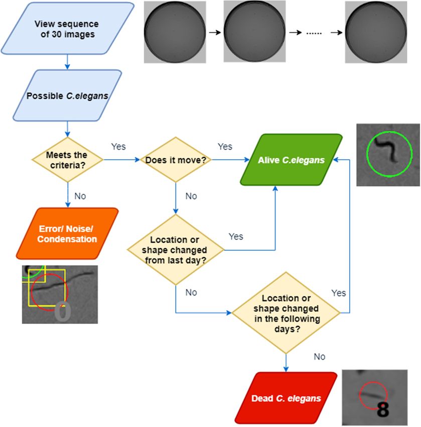
To carry
To carry out
outlabelling
labelling(Figure
(Figure6),6),the
the sequence
sequence of images
of 30 30 images
waswas
first first visualised,
visualised, and
and possible C. elegans were identified. Depending on whether they
possible C. elegans were identified. Depending on whether they met the nematodemet the nematode
charac-
characteristics (colour, length, width, and sinusoidal movement), they were analysed in
teristics (colour, length, width, and sinusoidal movement), they were analysed in detail.
detail. If the C. elegans moved during the 30-image sequence, it was labelled as alive.
If the C. elegans moved during the 30-image sequence, it was labelled as alive. If not, it was
If not, it was checked whether it was in the same position and posture on the previous
checked whether it was in the same position and posture on the previous and subsequent
and subsequent days. If no variation was observed, it was labelled as dead; otherwise, it
days. If no variation was observed, it was labelled as dead; otherwise, it was labelled as
was labelled as alive. As can be seen, this procedure is very laborious; hence, the cost of
alive. As can be seen, this procedure is very laborious; hence, the cost of generating a la-
generating a labelled dataset is high.
belled dataset is high.
Figure 6.
Figure 6. Flow
Flow chart
chart of
of the
the labelling
labelling process.
process.
The total number of labelled image sequences of each class is as shown in Table
Table 2.
2.Sensors 2021, 21, 4943 10 of 17
Table 2. Number of sequences of each class (alive/dead) in the original dataset.
Alive Dead
5696 847
This dataset, as demonstrated in the experiments and results section, was insufficient
for the neural network to learn to solve the proposed classification task. To solve this
drawback, different types of synthetic images were generated to increase the size of the
dataset. This work experimentally demonstrated that this increase in data helped to
improve the results.
The first types of synthetic sequences were generated with a C. elegans trajectory
simulator (Figure 7). This simulator is based on the following components: (a) set of real
images of empty Petri dishes; (b) real C. elegans trajectories obtained with a tracker stored in
xml files; (c) colour and width features obtained from real images; (d) random positioning
Sensors 2021, 21, 4943 algorithm of the trajectories within the dish; (e) static noise generator similar to the 11 of
one17
appearing in the original sequences.
Figure 7. Two
Figure 7. Two original
original image
imagesequences
sequencesare
areshown
shownon
onthe
theleft
leftand
and two
two sequences
sequences generated
generated byby
thethe simulator
simulator areare shown
shown on
on the right.
the right.
2.10. As
Neural Network Training
parameters, Method
the simulator received the number of sequences to be generated, the
numberThe of C. elegans
network was per plate, and the
implemented andspeed of the
trained movement
using (variation
the Pytorch between frame-
deep learning poses).
To make the network learn to detect small differences between poses,
work [32] on a computer with an Intel Core™ i7-7700K processor and NVidia GeForce
® the sequences that
were generated had small pose changes between the previous day’s pose
GTX 1070 Ti graphics card. The network was trained for 130 epochs using the cross-en- and the current
pose, whereas
tropy loss cost the subsequent
function day’s was
and Adam’s is the same
optimiser as theacurrent
[33] with learningday’s
ratepose. In addition,
of 0.0001 for 120
static blobs were added to these images, which also helped the network
epochs and 0.00001 for the last 10 epochs. The batch size chosen was 64 samples taking to distinguish C.
elegans
into from other
account memory darkconstraints.
blobs which Asmay appear in theand
a regularisation image.
dataLastly, small rotations
augmentation and
technique,
translations were applied to the images to simulate the displacements occurring
rotations (90°, 180°, and 270°) were used. The original images were resized to 224 × 224 when the
real plates were placed in the acquisition system. This simulator
pixels using bilinear interpolation to adapt them to the resnet input. allowed us to obtain the
number of sequences shown in Table 3.
2.11. Postprocessing
Table 3. Number of synthetic sequences of each class (alive/dead) generated with the simulator.
As discussed above, there are different situations (occlusions, dirt, decomposition,
reproduction, and aggregation)
Alive that can lead to errors in the dailyDead
live count of the lifespan
curve. To alleviate 11,220
these problems, the postprocessing algorithm proposed in [27] was
11,220
employed. This algorithm is based on the premise that lifespan curves must be monoton-
ically decreasing functions and, therefore, errors can be detected if the current day’s count
As shown
is higher than thein Table 2, the
previous number
day’s of dead C. elegans sequences was significantly lower
count.
thanThis
the number of live C. elegans. This
correction takes into account that is because there
in the first could
days theonly beare
errors onemost
sequence
likelyfor
to
each dead C. elegans, whereas, for the live sequence, there was the whole
be false negatives due to worm occlusions at the edge and aggregations, whereas, lifespan. Tointrain
the
last days, the errors are mostly likely due to false positives caused by plate dirt.
In this way, the lifespan cycle was divided into two periods. This division was made
on the basis of the mean life, which was usually 14 days for the N2 strain. In the first cycle,
the curves were corrected upwards, i.e., if the current day’s count was higher than the
previous day’s count, the previous day’s count was changed to the current value. In theSensors 2021, 21, 4943 11 of 17
the classifier, the number of samples in each class must be balanced; therefore, a large part
of the alive C. elegans sequences could not be used to train the network.
In order to take advantage of these remaining sequences, a second type of synthetic
image was designed. These consisted of replicating the image of a C. elegans, thus obtaining
a sequence of three images in which there was no movement or change in posture (dead
C. elegans sequence). Small translations and rotations were applied between frames to
simulate plate placement shifts.
2.10. Neural Network Training Method
The network was implemented and trained using the Pytorch deep learning frame-
work [32] on a computer with an Intel® Core™ i7-7700K processor and NVidia GeForce
GTX 1070 Ti graphics card. The network was trained for 130 epochs using the cross-entropy
loss cost function and Adam’s optimiser [33] with a learning rate of 0.0001 for 120 epochs
and 0.00001 for the last 10 epochs. The batch size chosen was 64 samples taking into account
memory constraints. As a regularisation and data augmentation technique, rotations (90◦ ,
180◦ , and 270◦ ) were used. The original images were resized to 224 × 224 pixels using
bilinear interpolation to adapt them to the resnet input.
2.11. Postprocessing
As discussed above, there are different situations (occlusions, dirt, decomposition,
reproduction, and aggregation) that can lead to errors in the daily live count of the lifespan
curve. To alleviate these problems, the postprocessing algorithm proposed in [27] was em-
ployed. This algorithm is based on the premise that lifespan curves must be monotonically
decreasing functions and, therefore, errors can be detected if the current day’s count is
higher than the previous day’s count.
This correction takes into account that in the first days the errors are most likely to be
false negatives due to worm occlusions at the edge and aggregations, whereas, in the last
days, the errors are mostly likely due to false positives caused by plate dirt.
In this way, the lifespan cycle was divided into two periods. This division was made
on the basis of the mean life, which was usually 14 days for the N2 strain. In the first cycle,
the curves were corrected upwards, i.e., if the current day’s count was higher than the
previous day’s count, the previous day’s count was changed to the current value. In the
second cycle, they were corrected downwards, i.e., the current day’s count was decreased
to the previous day’s value if it was lower.
2.12. Validation Method
To evaluate the proposed method, the available dataset was classified using the
following validation metrics:
• The confusion matrix (Table 4), showing the number of correct and wrong predictions
during model validation for each of the classes.
Table 4. Confusion matrix for our model.
Label Prediction Dead Prediction Alive
dead TD FA
alive FD TA
TD represents the actual (true) dead worms, FA represents the false live worms, FD
represents the false dead worms, and TA represents the actual (true) live worms.
• The hit ratio (Equations (1) and (2)), which measure the percentage of correct predic-
tions for a class out of all samples in that class.
TD
True dead rate = (1)
TD + FASensors 2021, 21, 4943 12 of 17
TA
True live rate = (2)
TA + FD
After evaluating the classification method, the error in the lifespan curves was tested
by calculating the error between the percentage survival of the manual count and the
automatic count. In addition, the results obtained were compared with those of the
traditional automatic computer vision algorithm used as a reference.
The percentage of live C. elegans on each day of the experiment was calculated using
Equation (3). The error in one day (e (d)) was the difference in absolute value between
the percentage of live C. elegans from the manual curve and the curve from the automatic
method (Equation (4)). The error per plate was the average of the errors over the days of
the experiment (Equation (5)).
live C. elegans current day
% live C. elegans = ×100 (3)
initial live C. elegans
e(d) = % live _manual(d) − % live _automatic(d) (4)
days
∑ e (d)
ep = d=1 (5)
days
The error per condition was calculated analogously, by adding up the count of all the
plates for that condition, calculating the survival rates, and averaging the absolute value of
the errors for each day.
3. Results
3.1. Initial Classification of the Original Dataset
First, the sequences of the original dataset (Table 2) were processed with the initial
detection algorithm (first stage of the classifier).
As Table 5 shows, 81.18% of the live C. elegans image sequences were classified by the
initial detection algorithm as a trivial live case. The remaining 18.82% were determined
by the initial detection algorithm to be C. elegans sequences to be classified by the neural
network. In the case of dead C. elegans, 1.65% of cases were misclassified.
Table 5. Results obtained by applying the initial detection algorithm to the original dataset.
Label Prediction Stationary/Noisy Prediction Alive
dead 833 14
alive 1072 4624
The sequences that were not classified as alive by the first stage of the classifier were
those used to build the training and validation dataset (Table 6) of the neural network.
Table 6. Size of the original training and validation datasets.
Dataset Sequences
Training 666
Validation 1000
3.2. Analysis of the NN Classifier Using Different Datasets
In this experiment, the described network was trained using (a) an original training
dataset taken from the original sequences that were not classified as alive in the previous
stage (1072 live sequences and 833 dead sequences), (b) a dataset generated with the
simulator (Table 3), and (c) a mixed dataset, consisting of the original images, those
generated by the simulator, and those generated by replicating images of live C. elegans.
However, all models were evaluated using the original validation dataset.Sensors 2021, 21, 4943 13 of 17
Since the number of sequences from each class had to be balanced, 833 sequences from
each class could be used, leaving 239 live sequences unused.
To build the original training and validation dataset (Table 6), it was considered that
at least a validation sample of 1000 sequences, i.e., 500 of each class, should be available.
Therefore, 333 images of each class remained to train the neural network.
The mixed dataset (Table 7) was formed using the images from the simulated dataset,
images from the original dataset, the original live images that were not used in order to
keep the dataset balanced (239), and the same number of dead images generated from the
live images.
Table 7. Mixed dataset.
Dataset Live Worm Sequences Dead Worm Sequences
Original 572 333
Simulated 11,220 11,220
Replicated - 239
Total 11,792 11,792
The results obtained (Table 8) when evaluating the different models with the original
validation dataset showed how using synthetic data improved the results by 10.40% and
how mixing original and synthetic data further increased the hit rates.
Table 8. Comparison of model accuracy when trained with different datasets and validated with the
original validation set.
Validation Validation
Training Training
True Dead True Live Mean Improvement
Dataset Size
Rate Rate
Original 666 78.60% 65.40% 72.00% -
Simulated 22,440 81.40% 83.40% 82.40% 10.40%
Mixed 23,584 86.00% 85.20% 85.60% 3.20%
Table 9 shows the confusion matrix obtained by validating the model trained with the
mixed dataset with the original dataset.
Table 9. Confusion matrix of the validation sequences classified by the neural network with the
model trained with a mixed dataset.
Label Prediction Dead Prediction Alive
Dead 430 70
Alive 74 426
3.3. Overall Accuracy Analysis of the Cascade Classifier
The confusion matrix of all C. elegans sequences classified by the proposed method,
i.e., live C. elegans classified at the initial detection stage (4624), and live and dead C. elegans
from the validation dataset classified by the network, is shown below (Table 10). The hit
ratio is shown in Table 11.
Table 10. Total confusion matrix.
Label Prediction Dead Prediction Alive
Dead 430 84
Alive 74 5050ratio is shown in Table 11.
Table 10. Total confusion matrix.
Label Prediction Dead Prediction Alive
Sensors 2021, 21, 4943 14 of 17
Dead 430 84
Alive 74 5050
Table 11.Final
Table11. Finalresults
resultsofofthe
thefull
fullclassification
classificationmethod
methodwith
withthe
thevalidation
validationdata.
data.
True Dead
True DeadRate
Rate True Live
True LiveRate
Rate Mean
Mean
83.66%
83.66% 98.56%
98.56% 91.11%
91.11%
3.4.Validation
3.4. Validationofofthe
theLifespan
LifespanMethod
Method
Inorder
In orderto toproperly
properlyvalidate
validatethetheautomatic
automaticlifespan
lifespanmethod,
method,ititwaswasnotnotenough
enoughtoto
analysethe
analyse thehit
hitratio
ratioofofthe
theclassifier;
classifier;indeed,
indeed,ititwas
wasnecessary
necessaryto tomeasure
measurethe thefinal
finalerror
erroronon
thelifespan
the lifespancurves.
curves.
For
For this
this purpose, aa lifespan
lifespanassay
assaywas wasperformed
performed with
with eight
eight plates
plates following
following the the
cul-
culture
ture andand acquisitionprocedures
acquisition proceduresdescribed
describedin in this
this article.
article. These plates
plates were
wereindependent
independent
of
ofthe
thedata
dataused
usedin inthe
thetraining
trainingand andvalidation
validationof ofthe
theclassification
classificationmethod.
method.EachEachplate
platehadhad
between
betweenninenineandand20 20C.C.elegans
elegansofofthe
theN2 N2strain,
strain,for totalofofnn==111.
foraatotal 111.
The
Themanual
manualcountcountperformed
performedfollowing
followingthe thelabelling
labellingmethod
methoddescribed
describedaboveabovewas was
taken
taken as ground truth. In addition to comparing the results of the proposed methodwith
as ground truth. In addition to comparing the results of the proposed method with
the
themanual
manualresults,
results,ititwas
wascompared
comparedwith withthetheautomatic
automaticmethod
methodproposed
proposedinin[27][27]totoobtain
obtain
aacomparison
comparisonwith withanother
anotherlifespan
lifespanautomation
automationmethod.method.
The
Thecurve
curveobtained
obtainedwith withthe proposed
the proposed method
method showed
showed an an
average
averageerror in the
error in analysis
the anal-
per plate of 3.54% ± 1.30%, while the traditional algorithm obtained
ysis per plate of 3.54% ± 1.30%, while the traditional algorithm obtained 3.82% ± 1.76%. 3.82% ± 1.76%. In the
In
analysis of the error per condition (Figure 8), an average error was obtained
the analysis of the error per condition (Figure 8), an average error was obtained on each on each day of
day of±2.30%
2.30% 2.31%, compared
± 2.31%, to 3.20%
compared to± 3.96%
3.20% for thefor
± 3.96% traditional algorithm.
the traditional algorithm.
Figure 8. Comparison of manual counting (blue curve), automatic counting traditional method
Figure 8. Comparison of manual counting (blue curve), automatic counting traditional method
(orange curve), and counting with the proposed method (grey curve). The horizontal axis shows
(orange curve), and counting with the proposed method (grey curve). The horizontal axis shows the
the days of the experiment, and the vertical axis shows the proportion of live C. elegans. Capture
days of the experiment,
was performed until dayand
21,the
andvertical axis shows
the remaining daysthe proportion
were C. elegans.
of liveusing
approximated Capture was
a Kaplan–Meier
performed
estimator. until day 21, and the remaining days were approximated using a Kaplan–Meier estimator.
A statistical significance analysis was carried out with the aim of (1) analysing the
differences between the manual curve and the curve obtained with the new method based
on neural networks, and (2) analysing whether the improvements obtained with the new
method with respect to the traditional automatic method were statistically significant.
The open-source tool OASIS [34] was used to perform the analysis. The results are
included in the Supplementary Materials.
As shown in Table S2 (Supplementary Materials), very similar results were obtained
for the manual and NN curves with a p-value of 0.7454.
When comparing the curve obtained with the traditional automatic method with the
curve obtained with the new method (NN), a p-value of 0.6075 was obtained; therefore, the
improvements were not statistically significant.Sensors 2021, 21, 4943 15 of 17
4. Discussion
This paper proposed a method to automate lifespan assays, which, by combining
traditional computer vision techniques with a neural network-based classifier, enables the
number of live and dead C. elegans to be counted, despite low-resolution images.
As mentioned above, detecting dead C. elegans is a complex problem, since, in the
last days of life, they hardly move, and these movements are only small changes in head
posture and/or tail movements. This is compounded by other difficulties such as dirt
appearing on the plate, hindering detection, and the slight displacements occurring when
the plates are placed in the acquisition system.
These difficulties mean that solving the problem using traditional techniques requires
image alignment in addition to manual adjustment of numerous parameters, making the
use of neural networks an attractive proposition.
By using our method based on neural networks, we avoid having to perform align-
ments and feature design. Despite the advantages of neural networks, they have the
difficulty of requiring large datasets to train them. In this work, we addressed this diffi-
culty by manually labelling a small dataset (108 plates) and applying data augmentation
techniques.
To generate a considerable increase in data, a simulator was implemented to scale the
initial training dataset (666 sequences) to a final dataset on the order of 23,000 sequences.
The results obtained showed that training the model with only the simulated dataset led to
an improvement in the hit ratio of 10.40% compared to the baseline of the model, trained
with the original dataset available. Furthermore, it was shown that training the model
with a mixed dataset of simulated and original data improved the hit ratio by a further
3.20%, reaching a 83.66% hit rate in the classification of dead C. elegans and a 98.56% hit
rate for live C. elegans. Errors in this method were mostly due to noise problems. These
errors included cases such as stains that merged with the worm body, stains that caused
the worm body to appear split, worm images in the border area, and worm aggregations.
Examples of such noise cases are presented in Figure S1 (Supplementary Materials).
Regarding the final error on the lifespan curves, the proposed method achieved small
error rates (3.54% ± 1.30% per plate) with respect to the manual curve, demonstrating
its feasibility and, moreover, with slightly better results than the traditional vision tech-
niques used as a reference. When obtaining the lifespan curves, several problems were
encountered. In the first days, worms could be lost due to occlusions in the plate walls
and aggregations; in the last days, false positives could occur due to plate soiling. These
problems were reduced by using an edge motion detection technique and a postprocessing
algorithm.
Supplementary Materials: The following are available online at https://www.mdpi.com/article/1
0.3390/s21144943/s1, Table S1: Survival analysis, Table S2: Log-rank test obtained with the open
source tool OASIS [34], Figure S1: Noise examples, Figure S2: N2 lifespan curve, Figure S3: Daf-2
lifespan curve.
Author Contributions: Conceptualisation, A.G.G. and A.-J.S.-S.; methodology, A.G.G. and A.-J.S.-S.;
software, A.G.G., J.C.P., P.E.L.C. and F.N.M.; validation, A.G.G.; formal analysis, A.G.G. and A.-
J.S.-S.; investigation, A.G.G. and A.-J.S.-S.; resources, A.-J.S.-S.; data curation, A.G.G., J.C.P., P.E.L.C.
and F.N.M.; writing—original draft preparation, A.G.G.; writing—review and editing, all authors;
visualisation, all authors; supervision, A.-J.S.-S.; project administration, A.-J.S.-S.; funding acquisition,
A.-J.S.-S. All authors read and agreed to the published version of the manuscript.
Funding: This study was supported by the Plan Nacional de I + D under the project RTI2018-094312-
B-I00 and by the European FEDER funds.
Institutional Review Board Statement: Not applicable.
Informed Consent Statement: Not applicable.
Data Availability Statement: We created a repository on github: https://github.com/AntonioGarc
iaGarvi/C.-elegans-alive-dead-classification-using-deep-learning (accessed on 19 July 2021) withSensors 2021, 21, 4943 16 of 17
a demo to show some examples of how our model classifies a C. elegans as alive or dead using a
sequence of three images corresponding to the current day, the day before, and the day after.
Acknowledgments: This study was supported by the Plan Nacional de I + D with Project RTI2018-
094312-B-I00 and by European FEDER funds. ADM Nutrition, Biopolis SL, and Archer Daniels
Midland provided support in the supply of C. elegans.
Conflicts of Interest: The authors declare no conflict of interest.
References
1. The C. elegans Sequencing Consortium. Genome Sequence of the Nematode C. elegans: A Platform for Investigating Biology.
Science 1998, 282, 2012–2018. [CrossRef]
2. Tissenbaum, H.A. Using C. elegans for Aging Research. Invertebr. Reprod Dev. 2015, 59, 59–63. [CrossRef] [PubMed]
3. Amrit, F.R.G.; Ratnappan, R.; Keith, S.A.; Ghazi, A. The C. elegans Lifespan Assay Toolkit. Methods 2014, 68, 465–475. [CrossRef]
4. Felker, D.P.; Robbins, C.E.; McCormick, M.A. Automation of C. elegans Lifespan Measurement. Transl. Med. Aging 2020, 4, 1–10.
[CrossRef]
5. Mathew, M.D.; Mathew, N.D.; Ebert, P.R. WormScan: A Technique for High-Throughput Phenotypic Analysis of Caenorhabditis
Elegans. PLoS ONE 2012, 7, e33483. [CrossRef]
6. Stroustrup, N.; Ulmschneider, B.E.; Nash, Z.M.; López-Moyado, I.F.; Apfeld, J.; Fontana, W. The Caenorhabditis Elegans Lifespan
Machine. Nat. Methods 2013, 10, 665–670. [CrossRef] [PubMed]
7. Churgin, M.A.; Jung, S.-K.; Yu, C.-C.; Chen, X.; Raizen, D.M.; Fang-Yen, C. Longitudinal Imaging of Caenorhabditis Elegans in a
Microfabricated Device Reveals Variation in Behavioral Decline during Aging. eLife 2017, 6, e26652. [CrossRef]
8. Puckering, T.; Thompson, J.; Sathyamurthy, S.; Sukumar, S.; Shapira, T.; Ebert, P. Automated Wormscan. F1000Res 2019, 6.
[CrossRef] [PubMed]
9. Pitt, J.N.; Strait, N.L.; Vayndorf, E.M.; Blue, B.W.; Tran, C.H.; Davis, B.E.M.; Huang, K.; Johnson, B.J.; Lim, K.M.; Liu, S.; et al.
WormBot, an Open-Source Robotics Platform for Survival and Behavior Analysis in C. elegans. GeroScience 2019, 41, 961–973.
[CrossRef]
10. Puchalt, J.C.; Layana Castro, P.E.; Sánchez-Salmerón, A.-J. Reducing Results Variance in Lifespan Machines: An Analysis of the
Influence of Vibrotaxis on Wild-Type Caenorhabditis Elegans for the Death Criterion. Sensors 2020, 20, 5981. [CrossRef] [PubMed]
11. Redmon, J.; Divvala, S.; Girshick, R.; Farhadi, A. You Only Look Once: Unified, Real-Time Object Detection. In Proceedings of the
2016 IEEE Conference on Computer Vision and Pattern Recognition (CVPR), Las Vegas, NV, USA, 27–30 June 2016; pp. 779–788.
[CrossRef]
12. Ren, S.; He, K.; Girshick, R.; Sun, J. Faster R-CNN: Towards Real-Time Object Detection with Region Proposal Networks. IEEE
Trans. Pattern Anal. Mach. Intell. 2017, 39, 1137–1149. [CrossRef]
13. Ronneberger, O.; Fischer, P.; Brox, T. U-Net: Convolutional Networks for Biomedical Image Segmentation. In Proceedings of the
Medical Image Computing and Computer-Assisted Intervention–MICCAI 2015; Navab, N., Hornegger, J., Wells, W.M., Frangi,
A.F., Eds.; Springer International Publishing: Cham, Switzerland, 2015; pp. 234–241.
14. Li, K.; Javer, A.; Keaveny, E.E.; Brown, A.E.X. Recurrent Neural Networks with Interpretable Cells Predict and Classify Worm
Behaviour. bioRxiv 2017. [CrossRef]
15. Hakim, A.; Mor, Y.; Toker, I.A.; Levine, A.; Neuhof, M.; Markovitz, Y.; Rechavi, O. WorMachine: Machine Learning-Based
Phenotypic Analysis Tool for Worms. BMC Biol. 2018, 16, 8. [CrossRef]
16. Bornhorst, J.; Nustede, E.J.; Fudickar, S. Mass Surveilance of C. elegans—Smartphone-Based DIY Microscope and Machine-
Learning-Based Approach for Worm Detection. Sensors 2019, 19, 1468. [CrossRef]
17. Javer, A.; Brown, A.E.X.; Kokkinos, I.; Rittscher, J. Identification of C. elegans Strains Using a Fully Convolutional Neural Network
on Behavioural Dynamics. In Proceedings of the Computer Vision–ECCV 2018 Workshops; Leal-Taixé, L., Roth, S., Eds.; Springer
International Publishing: Cham, Switzerland, 2019; pp. 455–464.
18. Mane, M.R.; Deshmukh, A.A.; Iliff, A.J. Head and Tail Localization of C. elegans. arXiv 2020, arXiv:2001.03981 [cs].
19. Chen, L.; Strauch, M.; Daub, M.; Jiang, X.; Jansen, M.; Luigs, H.; Schultz-Kuhlmann, S.; Krüssel, S.; Merhof, D. A CNN Framework
Based on Line Annotations for Detecting Nematodes in Microscopic Images. In Proceedings of the 2020 IEEE 17th International
Symposium on Biomedical Imaging (ISBI), Iowa City, IA, USA, 3–7 April 2020; pp. 508–512.
20. Hebert, L.; Ahamed, T.; Costa, A.C.; O’Shaughnessy, L.; Stephens, G.J. WormPose: Image Synthesis and Convolutional Networks
for Pose Estimation in C. elegans. PLoS Comput. Biol. 2021, 17, e1008914. [CrossRef]
21. Li, S.; Günel, S.; Ostrek, M.; Ramdya, P.; Fua, P.; Rhodin, H. Deformation-Aware Unpaired Image Translation for Pose Estimation
on Laboratory Animals. In Proceedings of the 2020 IEEE/CVF Conference on Computer Vision and Pattern Recognition (CVPR),
Seattle, WA, USA, 13–19 June 2020; pp. 13155–13165.
22. Lin, J.-L.; Kuo, W.-L.; Huang, Y.-H.; Jong, T.-L.; Hsu, A.-L.; Hsu, W.-H. Using Convolutional Neural Networks to Measure the
Physiological Age of Caenorhabditis Elegans. IEEE/ACM Trans. Comput. Biol. Bioinform. 2020. [CrossRef] [PubMed]
23. Wang, L.; Kong, S.; Pincus, Z.; Fowlkes, C. Celeganser: Automated Analysis of Nematode Morphology and Age. arXiv 2020,
arXiv:2005.04884 [cs].You can also read