UC Riverside UC Riverside Electronic Theses and Dissertations - eScholarship
←
→
Page content transcription
If your browser does not render page correctly, please read the page content below
UC Riverside
UC Riverside Electronic Theses and Dissertations

Title
Statistical Rate Event Analysis with Elite Sample Selection Scheme

Permalink
https://escholarship.org/uc/item/9nq6c5j6

Author
Zhao, Yue

Publication Date
2019

Peer reviewed|Thesis/dissertation

 eScholarship.org                                 Powered by the California Digital Library
                                                                  University of California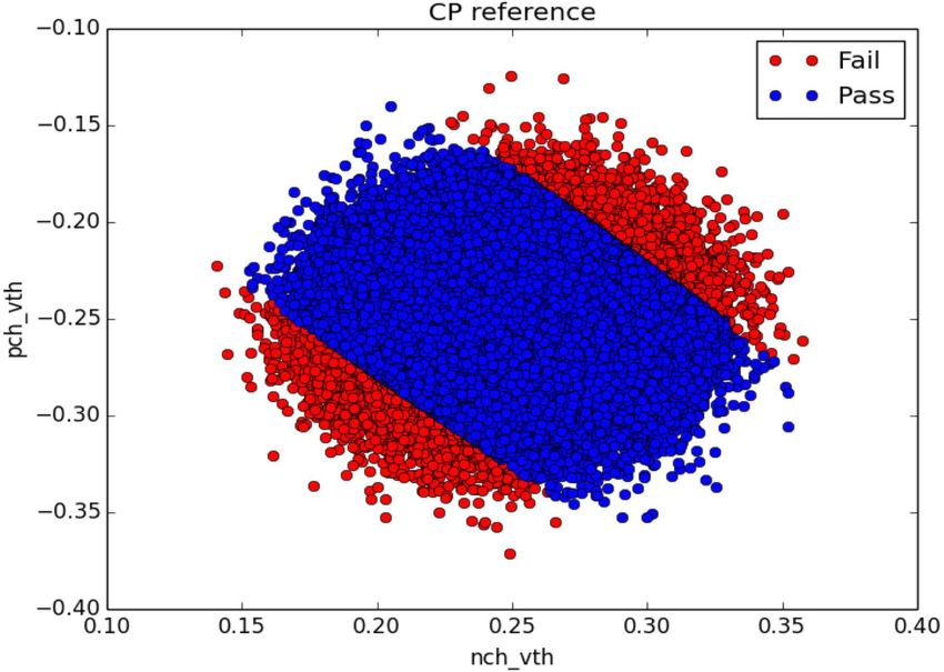
UNIVERSITY OF CALIFORNIA
                                 RIVERSIDE

       Statistical Rate Event Analysis with Elite Sample Selection Scheme

                 A Dissertation submitted in partial satisfaction
                      of the requirements for the degree of

                                Master of Science

                                         in

                              Electrical Engineering

                                         by

                                    Yue Zhao

                                 December 2019

Dissertation Committee:

    Dr. Sheldon X.-D. Tan, Chairperson
    Dr. Jianlin Liu
    Dr. Hyoseung Kim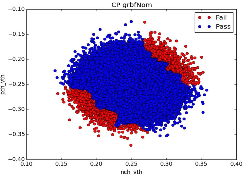
Copyright by
 Yue Zhao
   2019
The Dissertation of Yue Zhao is approved:

                                       Committee Chairperson

                University of California, Riverside
Acknowledgments
I am sincerely grateful to my advisor Dr. Sheldon X.-D. Tan for his continuous guidance,
and support. Throughout the graduate program, Dr. Tan spare no effort to help me on
financial and academic aspects. During my past few years I had the opportunity to build a
stronger understanding on EDA industry and machine learning area. I am also grateful to
have Dr. Jianlin liu and Dr. Hyoseung Kim as one of my dissertation committee members
for his invaluable advise and support. I would thank all of the members in VSCLAB. I had
a great time working with all current members and alumni. Thanks to for their friendship
and their help making me what I am today. Hope all of you have a good life and great
future. Finally, I could not have achieved this without my families. I would like to thank
my parents for raising me up with all of their care and unconditional love. Even though
we live in different country and had little time living together, we still care and love each
other. Proud of being your son!
ivTo my parents, Wendy and Emma.
vABSTRACT OF THE DISSERTATION
Statistical Rate Event Analysis with Elite Sample Selection Scheme
by
Yue Zhao
Master of Science, Graduate Program in Electrical Engineering
University of California, Riverside, December 2019
Dr. Sheldon X.-D. Tan, Chairperson
Accurately estimating the failure region of rare events for memory-cell and analog
circuit blocks under process variations is a challenging task. As the first part of the thesis,
author propose a new statistical method, called EliteScope to estimate the circuit failure
rates in rare event regions and to provide conditions of parameters to achieve targeted per-
formance. The new method is based on the iterative blockade framework to reduce the
number of samples. But it consists of two new techniques to improve existing methods.
First, the new approach employs an elite learning sample selection scheme, which can con-
sider the effectiveness of samples and well-coverage for the parameter space. As a result,
it can reduce additional simulation costs by pruning less effective samples while keeping
the accuracy of failure estimation. Second, the EliteScope identifies the failure regions in
terms of parameter spaces to provide a good design guidance to accomplish the performance
target. It applies variance based feature selection to find the dominant parameters and then
determine the in-spec boundaries of those parameters. We demonstrate the advantage of
our proposed method using several memory and analog circuits with different number of
viprocess parameters. Experiments on four circuit examples show that EliteScope achieves a
significant improvement on failure region estimation in terms of accuracy and simulation
cost over traditional approaches. The 16-bit 6T-SRAM column example also demonstrate
that the new method is scalable for handling large problems with large number of process
variables.
viiContents
List of Figures x
List of Tables xi
1 Introduction 1
1.1 Introduction of Statistical Rare Event Analysis . . . . . . . . . . . . . . . . 1
1.2 Motivation . . . . . . . . . . . . . . . . . . . . . . . . . . . . . . . . . . . . 3
1.3 Contributions and Outline of the Thesis . . . . . . . . . . . . . . . . . . . . 5
2 Background Knowledge of Statistical Rare Event Analysis 7
2.1 Existing Sampling Approaches . . . . . . . . . . . . . . . . . . . . . . . . . 7
2.1.1 Importance Sampling . . . . . . . . . . . . . . . . . . . . . . . . . . 7
2.2 Statistical Blockade . . . . . . . . . . . . . . . . . . . . . . . . . . . . . . . . 8
2.2.1 Classification . . . . . . . . . . . . . . . . . . . . . . . . . . . . . . . 9
2.2.2 Failure probability calculation . . . . . . . . . . . . . . . . . . . . . . 10
2.3 Recursive Statistical Blockade . . . . . . . . . . . . . . . . . . . . . . . . . . 12
3 Proposed Elite Sample Selection Scheme Method 15
3.1 The Overall Analysis Flow of EliteScope . . . . . . . . . . . . . . . . . . . . 15
3.1.1 Elite Learning Sample Selection . . . . . . . . . . . . . . . . . . . . 17
3.1.2 Parameters Guidance for Performance Targeting . . . . . . . . . . . 20
4 Numerical Experimental Results 23
4.1 Experiment Configuration . . . . . . . . . . . . . . . . . . . . . . . . . . . . 23
4.1.1 The Critical Path Delay of the Simple Logic Circuit . . . . . . . . . 24
4.1.2 Failure Rate Diagnosis of Single-bit 6T-SRAM Cell . . . . . . . . . . 26
4.1.3 Charge Pump Failure Rate Diagnosis . . . . . . . . . . . . . . . . . . 29
4.1.4 16-bit 6T-SRAM Column Failure Rate Diagnosis . . . . . . . . . . . 32
4.1.5 Classifier Computation Complexity and Performance Convergence Anal-
ysis . . . . . . . . . . . . . . . . . . . . . . . . . . . . . . . . . . . . 35
5 Conclusions and Future Research 38
viiiBibliography 40
ixList of Figures
2.1 Generated PDF by importance sampling in 2-D random variables . . . . . . 8
2.2 General flow of statistical blockade approach . . . . . . . . . . . . . . . . . 9
2.3 The classification accuracy of two different methods . . . . . . . . . . . . . 10
2.4 Iterative locating of failure region by changing thresholds . . . . . . . . . . 13
3.1 The proposed iterative failure region diagnosis flow . . . . . . . . . . . . . . 16
3.2 Sample candidates weight Distribution of a single-bit SRAM test . . . . . . 19
3.3 Overall flow of parameters guidance for performance targeting 1) Feature
selection 2) Sampling and Classification 3) Calculate the boundaries for in-
spec conditions . . . . . . . . . . . . . . . . . . . . . . . . . . . . . . . . . . 22
4.1 The schematic of the 4-gates logic circuit . . . . . . . . . . . . . . . . . . . 24
4.2 The failure distribution P(Y< tc )=0.999875 of the critical path delay of the
simple circuit . . . . . . . . . . . . . . . . . . . . . . . . . . . . . . . . . . . 25
4.3 The schematic of the 6T-SRAM single-bit cell . . . . . . . . . . . . . . . . . 26
4.4 Estimating the CDF of the 6T-SRAM read time around 3-sigma region . . 27
4.5 A functional diagram of the PLL circuit . . . . . . . . . . . . . . . . . . . . 29
4.6 Schematic representations of the charge pump and filter . . . . . . . . . . . 30
4.7 Estimating the CDF of charge pump mismatch around 3-sigma region . . . 31
4.8 The schematic of a 16-bit 6T-SRAM column . . . . . . . . . . . . . . . . . . 32
4.9 Estimated Failure Threshold Error of RSB and EliteScope . . . . . . . . . . 36
4.10 Relative Failure Threshold Error of RSB and EliteScope . . . . . . . . . . . 37
xList of Tables
4.1 Process parameters of MOSFET . . . . . . . . . . . . . . . . . . . . . . . . 24
4.2 Comparison of the accuracy and efficiency on the 4-gates circuit . . . . . . 25
4.3 Comparison of the accuracy and efficiency on the 6T-SRAM circuit . . . . . 27
4.4 Estimated in-spec guidance of parameters on the 6T-SRAM circuit . . . . . 28
4.5 Comparison of the accuracy and efficiency for the charge pump circuit . . . 31
4.6 Estimated in-spec guidance of parameters for the charge pump circuit . . . 32
4.7 The accuracy comparisons for 16-bit 6T-SRAM column case . . . . . . . . . 34
xiChapter 1
Introduction
1.1 Introduction of Statistical Rare Event Analysis
As VLSI technology scales into the nanometer regime, chip design engineering face
several challenges in maintaining historical rates of performance improvement and capacity
increase with CMOS technologies. One profound change in the chip design business is that
engineers can’t put the design precisely into the silicon chips. Chip performance, manu-
facture yield and lifetime become unpredictable at the design stage. Chip performance,
manufacture yield and lifetime can’t be determined accurately at the design stage. The
main culprit is that many chip parameters – such as oxide thickness due to chemical and
mechanical polish (CMP) and impurity density from doping fluctuations – can’t be deter-
mined precisely, and thus are unpredictable. The so-called manufacture process variations
start to play a big role and their influence on the chip’s performance, yield and reliability
becomes significant.
1As a result, how to efficiently and accurately assess the impacts of the process
variations of interconnects in the various physical design steps are critical for fast design
closure, yield improvement, cost reduction of VLSI design and fabrication processes. The
design methodologies and design tools from system level down to the physical levels have to
embrace variability impacts on the VLSI chips, which calls for statistical/stochastic based
approaches for designing next generation VLSI systems.
Moreover, the performance uncertainties related to the process variation have be-
come a major concern for IC development [2]. Many IC components such as SRAM bit-cells
need to be tremendously robust as they are duplicated in the millions [8]. Such modules
require accurate statistical failure analysis in rare event region. However, the traditional
Monte Carlo (MC) based statistical analysis method faces a challenge as it may require
millions of simulations [14].
In this regard, it is imperative to develop new design methodologies to consider
the impacts of various process and environmental uncertainties and elevated temperature on
chip performance. Variation impacts and thermal constraints have to be incorporated into
every steps of design process to ensure the reliable chips and profitable manufacture yields.
The design methodologies and design tools from system level down to the physical levels
have to consider variability and thermal impacts on the chip performance, which calls for
new statistical and thermal-aware optimization approaches for designing manometer VLSI
systems.
21.2 Motivation
To mitigate this problem, a number of statistical analysis algorithms have been
developed in the literature [4, 15, 19, 20, 14, 9, 1, 11, 12]. One way is by means of
importance sampling (IS) [4], which consist of two steps. First, it shifts the mean value of
the initial performance distribution and places it on interested failure region. The standard
deviation based on the shifted mean is recalculated by considering samples only placed
on the failure region. The new probability density function (PDF) is generated based on
updated mean and standard deviation so that more samples in the failure region can be
drawn. Work in [12] applied the mixture of IS for cross-validation of multiple failure regions
due to disjointed process parameters.
However, these approaches can only estimate single performance metric. Multiple
important samplings are required to estimate more metrics. Also, it is difficult to calculate
the failure probability for a generated distribution by IS.
The statistical blockade (SB) is another effective approach for improving the per-
formance of MC method [14]. The idea of this approach is using a threshold bound to
separate an interested failure region from the whole distribution so that it can block some
unnecessary sampling and simulation for efficiency improvement. This method builds a
supervised learning model with the threshold bound and initial simulation data, which is
known as “classifier”, to recognize failure samples. Later samples that tend to be placed in
the failure region can be captured without simulation.
This approach was improved by using the recursive statistical blockade (RSB)
scheme to locate the rare event failure region in an iterative way [15]. This iterative method
3can improve the accuracy of the classifier by increasing the number of samples in the failure
region of interest. However, this method can incur the significant extra cost as it needs
more samples for the simulation. Wu et al. [20] applied a nonlinear SVM (Support Vector
Machine) classifier to model nonlinear and multiple disjoint failure regions of circuits. This
method applies the generalized Pareto distribution (GPD) fitting for tail distribution to
model failure probability in each iteration. However, this method cannot further investi-
gate failure region without rerunning the whole algorithm. The reason is that the pruned
parameters depending on the initial samples cannot be remained as important ones in the
failure region, which keeps changing. Also, the previous approaches cannot provide the
design guideline in terms of the design parameters to explicitly avoid performance failure,
which are important for improving the yield of circuit.
Recently, Sun et al. proposed scaled-sigma sampling (SSS) [16] and subset sim-
ulation technique (SUS) [17] as better solutions to estimate rare failure rates with high-
dimensional variation space. Unlike traditional importance sampling (IS), SSS applied soft
maximum theorem to construct an analytical model, which is insensitive to dimensionality,
for rare failure rate estimation. Subset simulation (SUS), on the other hand, tends to ex-
press rare failure probability as a product of conditional probability of intermediate failure
events, which is similar to the recursive statistical blockade concept. These intermediate
terms are then accurately estimated using MCMC (Markov Chain Monte Carlo) algorithm.
41.3 Contributions and Outline of the Thesis
In this thesis, the author proposes a new statistical failure region diagnosis method.
The new method, called EliteScope, is based on recursive statistical blockade method to
reduce the sample counts while still maintaining estimation accuracy. But, it consists of
two new techniques to improve existing methods. The main contribution of this paper
article are as follows:
Firstly, in the recursive statistical blockade method, more samples will be gener-
ated when the failure region is redefined gradually. To mitigate these problems, the new
approach applies an elite sampling scheme, which considers both effectiveness of samples
and well-coverage for process parameter search space, to reduce the number of generated
samples after the failure regions are relocated.
Secondly, our approach provides safe boundaries or in-spec boundaries of process
parameters to satisfy the design specification and manage yield variability of circuit. The
new method first applies variance based feature selection to find the dominant parameters.
A quasi-random sampling with dominant parameters is then used to quickly determine
proper boundaries of those parameters.
The presented method has been tested on several types of digital and analog/mixed-
signal circuits: 4-gate logic circuit with 48 process parameters; a charge pump operation
failure diagnosis in a PLL circuit with 81 process parameters; 6T-SRAM reading failure
diagnosis with 27 process parameters; 16-bit 6T-SRAM column reading failure diagnosis
with 432 process parameters. Experimental results show that given the same computing
costs, the proposed method in general can be more accurate than all the existing methods.
5For instance, for the 16-bit 6T-SRAM column, with the similar number of samples used,
EliteScope can deliver about 3-10X accuracy improvement over existing method. Further-
more, the 16-bit 6T-SRAM column example also shows that the new method can easily
handle the statistical analysis problems with large number of process variables.
The rest of this paper is organized as follows. Chapter 2 discusses essential back-
ground for sample-based failure analysis and revisits some important techniques for im-
proving MC performance. In Chapter 3, we first introduce an overall flow of the proposed
method and review of the mathematical framework for recursive statistical blockade based
method. We then present the proposed elite sampling method to reduce the number sam-
ples for efficiency improvement. We then introduce new guidance technique of parameters
to meet target performance. Chapter 4 shows the experimental result for verifying the ac-
curacy and efficiency of the proposed method. Computation complexity and convergence
performance analysis of EliteScope is also discussed. Chapter Conclusion will highlight the
author‘s contribution wrap-up this thesis.
6Chapter 2
Background Knowledge of
Statistical Rare Event Analysis
2.1 Existing Sampling Approaches
2.1.1 Importance Sampling
In sample-based statistical analysis, importance sampling (IS) is a general tech-
nique to estimate properties of rare event region using the samples generated from the
initial distribution. Fig. 2.1 shows the generated distribution g(x) by IS with two param-
eters. As we can see in the figure, the property of the failure region can be captured as
more samples are obtained in the failure region. Therefore, the proper sampling scheme is
needed to build the right distribution representing the rare event region. One of IS-based
approaches is focusing on quasi-random sampling to explore the parameters space more
uniformly. The samples can be selected by the initial MC sampling, so that more regular
7Probability x2
g(x2)
f(x1)
f(x) g(x)
g(x1)
f(x2)
g(x2)
g(x1)
Y x1
Figure 2.1: Generated PDF by importance sampling in 2-D random variables
space filling makes the initial samples to cover large variety combinations of parameters
[3]. Another well-known approach is the mean shifting and variance reconstructing, which
the initial distribution is centered around the failure region [12, 11]. However, all these
approaches assume a linear relation between the reconstructed and the initial distributions,
so the generated samples cannot reflect the nonlinear rare event region correctly.
2.2 Statistical Blockade
We first briefly review the concept of the statistical blockade (SB) approach for fast
estimation of properties of rare event region. A general framework of SB is shown in Fig. 2.2.
This method starts with drawing initial samples with uniform or normal distribution to
capture a crude shape of performance distribution by circuit simulation. The classifier can
be built by training with initial simulation data. Once we obtain the classifier, samples
that tend to fall into the failure criteria can be identified without actual simulation. With
these filtered samples, SB calculates the probability of failure region by fitting samples in
8x2
. .... . . ..!..
. .. .. ! . . . .. . .. ... .. ! ! . ...
... . ...! . . .. .. .. . .... .. !. .. .....
.....
fail region .. .. .. .. ... ... . .. .. .. ...... . .
. Fitting
. .... .... .. !.
....... . .. .. .. ... !. . .x1 !.
.. .. .. . .. . . .. ... . . !. !!.
.......... . . . .! . !!.
. .!. .. .. . .. ... ... .. .. .. ! !!!!
................ . .. . !!!!
. . .. .... . .. !!!!!!!!.
y !. ! .. .... ... ...... .. ... !!!!!!!!.
. ! . .. . .. .. .. .. . . .. y
Initial sampling and
simulation Doing “classification” Fitting failure region to
distribution
Figure 2.2: General flow of statistical blockade approach
proper distribution model. Thus, “classification” and “failure probability calculation” are
both key steps in the SB method. The rest of this section describes these two steps.
2.2.1 Classification
The classification is a step that the samples can be classified into likely-to-fail sam-
ples for circuit simulation. Building a classifier needs a training step with initial samples
to render real shapes of the failure region. The classifier can shrink the number of samples,
thus the simulation cost is reduced. However, it is not capable of fully replacing the simu-
lator due to its accuracy. So, a marginal filtering approach is used to improve the accuracy
of classification [15, 19, 20, 14]. This method uses relaxed threshold bounds instead of a
real failure criterion to capture more samples to minimize classification error. Meanwhile,
it is not sufficient to use a simple and linear classifier due to the nonlinearity of the failure
region [15, 19, 14]. So, Gaussian radial basis function kernel (GRBF) and neural network
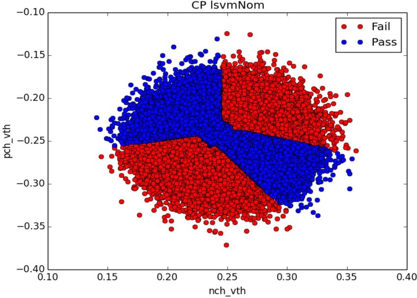
methods are available for nonlinear classifiers [20, 18]. Fig. 2.3 shows the accuracy of classi-
fication in a 2-dimensional search space example. Even the solution space is separated with
9(a) Reference (b) GRBF (c) LSVM
Figure 2.3: The classification accuracy of two different methods
nonlinear relation, GRBF can recognize patterns properly while the LSVM draws a wrong
boundary between two categories.
2.2.2 Failure probability calculation
The failure samples should be fitted to a particular distribution form in order
to calculate the probability of the failure region. Suppose that simulation results for the
certain performance metric Y can be fitted to the Gaussian distribution. The PDF of the
result distribution can be represented as
1 (y−µ)2
f (y, µ, σ) = √ e− 2σ2 (2.1)
σ 2π
where parameters µ and σ are the mean and standard deviation in this distribution. We
define FY (y) as the cumulative density function (CDF) of the performance metric Y . If we
know the threshold value t which separates a tail region from the whole distribution f (y),
the conditional CDF of this region can be written as follows:
FY (y) − FY (t)
Ft (y) = P (Y ≥ y | Y ≥ t) = (2.2)
1 − FY (t)
10where Ft (y) means the failure probability decided by y. Once we have a suitable fitting
model for CDF of the failure region with a failure bound y, the failure probability with
given values can be calculated as:
P (Y ≥ y) = [1 − FY (t)] · [1 − Ft (y)] (2.3)
In the several generalized extreme value distributions, GPD is one of the most accurate
model to describe tail distribution corresponding to failure region [7]. With the location
parameter µ, the scale parameter σ and the shape parameter ξ, CDF of the failure region
can be formulated by GPD fitting.
Ft (y) = G(ξ,µ,σ) (y)
−1/ξ
1 − 1 + ξ(y − µ) (2.4)
for ξ 6= 0
σ
=
−(y−µ)
1 − e σ
for ξ = 0
The location parameter µ means a starting point of GPD and it corresponds to the threshold
t of the tail distribution. Consequently, the failure probability with given threshold t and
failure bound y can be computed as follows.
P (Y ≥ y) = [1 − FY (t)] · [1 − G(ξ,t,σ) (y)] (2.5)
To approximate the rest of parameters for GPD fitting, we use the maximum likelihood
estimation [6].
112.3 Recursive Statistical Blockade
It is a typically difficult task to choose the right threshold bound in the failure
analysis for an extreme rare event region. For instance, the failure region is decided by the
failure criterion tc and the probability of this region is around 99.9999%. Suppose that we
use single threshold method, then we can choose a very loose threshold t as P (Y > t) around
99% to safely cover whole failure region even though the threshold can be quite far away tc .
Moreover, the number of MC samples for filtering will be determined at once. If the number
of MC samples is relatively enormous, a classifier will select too many likely-to-fail samples,
which will significantly increases simulation cost. Meanwhile, if the selected likely-to-fail
samples is every small, this will cause inaccurate estimation of the failure region and thus
the failure probability.
To mitigate this problem, one idea is to gradually locate the failure region in an
iterative way based on RSB scheme [15]. Unlike the single threshold method that calculates
a failure probability at once, our approach updates a failure region Y1 (> 99%) and the
probability by GPD fitting after the first iteration. With this updated failure region, the
threshold bound is re-computed for a newly updated region Y2 (> 99.99%). The GRBF
classifier is trained by failure samples in the first iteration so that it can capture likely-
to-fail samples more precisely in the updated failure region. In the second iteration, the
number of MC samples increases from 10n to 102 n as the increasing ratio is 10, so the new
classifier will capture more likely-to-fails samples thus better estimating the updated failure
region.
121st zooming 2nd zooming i-th zooming
T(1) TC T(1) T(2) TC T(i-1) T(i)TC
Initial
sampling (n)
Y Y Y
Figure 2.4: Iterative locating of failure region by changing thresholds
As the algorithm iterates, the failure region is scoped continuously close to the
given failure criterion tc based on the re-computed ti and likely-to-fail samples are converged
on the updated failure region. Therefore, the proposed method can achieve accurate failure
analysis than a single threshold method with relatively less total simulation cost. Fig. 2.4
shows an iterative locating procedure for finding the failure region.
Mathematically, as discussed in Section 2.1, the CDF with given a threshold t and
a failure criterion tc can be calculated as
PIS (Y ≥ tc ) = PM C (Y ≥ t) · P (Y ≥ tc |Y ≥ t)
(2.6)
P (Y ≥ tc , Y ≥ t)
P (Y ≥ tc |t ≥ t) =
P (Y ≥ t)
The conditional probability part in (2.6) can be estimated by GPD fitting using simulated
failure samples. Therefore, (2.6) can be rewritten as
PIS (Y > tc ) = PM C (Y ≥ t) · PM IS (Y ≥ tc |Y ≥ t) (2.7)
where PM IS represents the conditional probability in updated distribution by GPD fitting.
If the proposed method iterates twice with t1 and t2 as threshold bounds, the second failure
probability can be calculated based on the first failure region. So, the failure probability in
13each step can be calculated as
PIS (Y ≥ tc ) = PIS(2) (Y ≥ tc )
PIS(1) (Y ≥ t2 ) = PM C (Y ≥ t1 )
· PM IS(1) (Y ≥ t2 |Y ≥ t1 )
(2.8)
PIS(2) (Y ≥ tc ) = PM C (Y ≥ t1 ) · PM IS(1) (Y ≥ t2 )
· PM IS(2) (Y ≥ tc |Y ≥ t2 )
PM IS(i) (Y ≥ tc )
PM IS(i) (Y ≥ tc |Y ≥ ti ) =
PM IS(i) (Y ≥ ti )
Without the loss of generality, we can formulate the iterative failure probability calculation
as
PIS(i) (Y ≥ tc )
PM C (Y ≥ ti ) · PM IS(i) (Y ≥ tc |Y ≥ ti ) for i = 1
(2.9)
k−1
Y
= PM C (Y ≥ ti ) · (PM IS(i) (Y ≥ ti+1 )
i=1
· PM IS(k) (Y ≥ tc |Y ≥ tk )) for i > 1
where k is the number of iterations. Finally, the failure probability can be obtained by
combining all calculated probabilities in each iteration.
14Chapter 3
Proposed Elite Sample Selection
Scheme Method
3.1 The Overall Analysis Flow of EliteScope
In this subsection, we first present the overall analysis flow of the proposed EliteScope
method, which is illustrated in Fig. 3.1. Then we present the mathematical framework for
the iterative computing of failure probability. Then we explain our three major contri-
butions of the proposed method: (1) Iterative computing of failure probability (2) Elite
learning sample selection (3) Parameters guidance for performance targeting.
Our algorithm starts with given data, such as process variations and some param-
eters for failure region determination. The failure criteria tc denotes the reference value of
failure and the percentile bound p to calculate the threshold in each ith iteration. The first
step is to perform initial MC sampling and simulation to capture overall circuit performance
15Process Variation Parameters
Failure criteria (tc)
Percentile bound to calculate threshold (p)
Initial MC sampling (n)
and circuit simulation
Update percentile bound p=pi
Calculate threshold ti for P(Y>ti)=p
Building classifier C(n,ti)
MC sampling (n=n*mi)
Calculating
Filtering likely-to-fail samples by C(n,ti)
In-of-specifications of
process parameters
Smart sample selection
[MIN,MAX] boundaries
of process parameters Circuit simulation
Update failure probability and region Y(ti)
N
ti > tc
Y
Failure probability
P(Y>tc) estimation
Termination
Figure 3.1: The proposed iterative failure region diagnosis flow
metrics. After this, the relaxed threshold ti can be obtained to separate a failure region from
main PDF and the probability of this region is P (Y > ti ) = p. The classifier can then be
modeled with n simulation result of the initial samples. In the classification step, the GRBF
nonlinear classifier is used for accurate sample filtering. With the simulation result and the
classifier, the new method can calculate the in-spec conditions of process parameters to
achieve targeted yield in ith iteration. At the same time, the algorithm generates n ∗ mi (m
is a constant number) MC samples, which will be filtered by the classifier Ci to likely-to-fail
samples based on ti . Then, the elite sample selection can be employed to further reduce
16the number of samples for actual simulation. After the simulation, the failure probabilities
P (Y > ti ) are updated by GPD fitting. Our approach iterates the above whole procedure
with the updated threshold bound ti by percentile bound p, and the increased number of
MC samples to calculate the failure probability P (Y > ti ). Finally, it finishes when the
threshold bound meets the given failure criterion tc .
3.1.1 Elite Learning Sample Selection
The simulation cost is a major bottleneck in the statistical analysis of the circuit.
The proposed iterative failure diagnosis method can lead to an extra simulation cost in each
iteration. To mitigate this problem, we propose the elite learning sample selection scheme,
which significantly reduces the number of samples required. The elite sample selection
process is represented in the box named “Smart sample selection” in Fig. 3.1. Effectiveness
of the sample group is the first factor. Each sample consists of the combination of process
parameters, which affect differently on simulation results. Therefore, the sensitivity of each
parameter should be considered for the sample selection.
Suppose we have a set of n samples, which are represented by the parameter vectors
xi , i = 1, ..., n. Each sample has m process variables (m dimensions). Together they form
a process parameter matrix X = [x1 x2 ... xn ] such that each column indicates a xi .
It is not difficult to see that each row of X is the n samples of a single parameter. Denote
X j as the vector formed from the jth row of X (jth process variable). A scalar vector
y = [y1 , y2 , ..., yn ]T contains all the corresponding n simulation results. σX j and σY are
variances of X j and y, respectively. The proposed selection method calculates correlation
coefficients between parameters and simulation results for the sensitivity analysis as follows:
17X j , y ∈ Rn
cov(X j , y)
ρX j ,y = j = 1, 2, ..., m (3.1)
σX j σy
ρX,y = [ρX 1 ,y ρX 2 ,y ... ρX m ,y ]T ∈ Rm
Where ρX,y means the co-variance coefficient of simulation results and m process parame-
ters.
The second factor is the coverage ratio of parameters search space by selected
samples. The diversity of samples can be calculated by Euclidean distances with the ref-
erence sample, which is the median from simulation results. Samples around the median
can be chosen as the median is located on the highest probability region in the distribution
of simulation results. Simultaneously, samples found in the boundary region of the search
space can be selected as these samples represent the maximum and minimum conditions of
parameters. Thus, the proposed sampling method can calculate two distance factors of a
given sample that covers both central and boundary regions of the search space as follows:
ỹ = median(y)
xref = {x|ỹ = f (x), x ∈ Rm }
1 (3.2)
Dcentral (x) = ∈ Rm
x−xref
Range(X)
x − xref
Dboundary (x) = ∈ Rm
Range(X)
where Range(X) is a normalization term such that the jth element of vector x − xref is
normalized by |max(X j ) − min(X j )|, the value range of jth row in X . In (3.2), Dcentral
increases when the sample is closer to the reference sample. On the other hand, Dboundary
increases. Since D(x) and ρX,y means the distance and correlation coefficient in same
dimensions, we can obtain the sample’s weight by the inner product of ρX,y and D(x) of
181.0
Normalized weight distribution in Wcentral
0.8
0.6
0.4
0.2
0.00 200 400 600 800 1000 1200
1.0
Normalized weight distribution in Wboundary
0.8
0.6
0.4
0.2
0.00 10 20 30 40 50
Figure 3.2: Sample candidates weight Distribution of a single-bit SRAM test
each sample.
Wcentral (x) = ρX,y T · Dcentral (x)
(3.3)
T
Wboundary (x) = ρX,y · Dboundary (x)
According to the selection ratio r, which determines the number of selected samples, The
final set of samples can be chosen in the following way.
nr nr (3.4)
E(n, r) = S( , Wcentral (xn )) ∪ S( , Wboundary (xn ))
2 2
where S(n, W (xn )) is the set of n samples sorted by W (xn ).
An example of normalized sample candidates weight distribution is shown in
Fig. 3.2. Nearly 1200 sample candidates are filtered out by the non-linear SVM classi-
fier. By employing Elite Learning Sample Selection scheme, the weight concerning both
19central and boundary distance are calculated sorted in descending order. All weights in the
same set are then normalized by sets maximum. For the normalized weight distribution in
the set Wboundary , only first 50 samples are listed since rest samples‘ weight are very close
to zero and thus negligible. It is very clear to see that weight values decease dramatically.
According to previous discussion, sample with larger weight leads to more significant con-
tribution in constructing the failure region. Unlikely to traditional RSB [15] method which
directly simulates all sample candidates, we only need to utilize samples with larger weight
to perform actual simulation to estimate failure region with great efficiency.
3.1.2 Parameters Guidance for Performance Targeting
In order to improve yield of a circuit, designers need to know good ranges of process
parameters with regards to the circuit performance specification. However, applying all
possible combinations of parameters is impossible due to exponential possibilities with a
large number of parameters.
The proposed method ranks priorities of process parameters based on its variances.
The parameter guidance operation is represented by the two left boxes in Fig. 3.1. Since
the parameters with huge variance mainly lead to spread samples in search spaces, these
parameters must be handled to avoid certain failure regions. In Fig. 3.1, the variances
of parameters can be calculated from simulation data of updated failure region in our
iterative framework. Given n samples with m process parameters as denoted by X =
[x1 x2 ... xn ], the variance of samples can be written mathematically as follows:
n
1X
V ar(X) = (xi − µ)2 (3.5)
n i=1
20where xi is a ith X and µ is the mean vector of n samples of X. Next, our method redraws
samples with only considering the distributions of high ranked parameters. Nominal values
are assigned for not chosen parameters. We use SOBOL sequence [5] to redraw these
samples. It uses a quasi-random low-discrepancy sequence, so these samples can cover
the search spaces of parameters more uniformly than the previous samples for simulation.
Suppose that l is the number of redrawn samples and first k high ranked parameters are
chosen. Redrawn samples can be formed as
xi = [xi,1 , xi,2 , ..., xi,k , xi,(k+1) , ...xi,m ]T ∈ Rm
[xi,1 , xi,2 , ..., xi,k ] = SOBOL[x1,...l , M IN (x1,...,l ), M AX(x1,...,l )] (3.6)
[xi,(k+1) , xi,(k+2) , ...xi,m ] = N OM IN AL(x1,...l )
where i = 1, 2, ..., l, xi,k denotes the kth element of xi , terms M IN (x1,...,l ) and M AX(x1,...,l )
mean the minimum and the maximum values of l vectors in X, respectively. We assign
nominal values for rest m − k parameters of redrawn samples. As a result, we can generate
samples with not only reduced dimensions but also well-coverage of the failure region. The
classifier with the updated threshold can filter out these samples to determine pass or fail
condition of process parameters. With the classification result of samples, the proposed
method induces if-then rules from the highest-ranked parameters so that all failure condi-
tions of parameters can be filtered. The overall steps of the new in-spec guidance method
are explained in Fig. 3.3.
21Sampling by SOBOL sequence Binary decision based on priority
Simulation
nth0
data
out-spec In-spec
Variance-based tox !
Feature tox
Selection out-spec In-spec
nth0
Rank Parameters pth0 pth0
1 nth0 Classification
2 tox
3 pth0 Classification In-spec guidance
4 Cgs
result of parameters
! !!
Figure 3.3: Overall flow of parameters guidance for performance targeting 1) Feature selec-
tion 2) Sampling and Classification 3) Calculate the boundaries for in-spec conditions
22Chapter 4
Numerical Experimental Results
4.1 Experiment Configuration
The proposed method (EliteScope) has been implemented in Python 2 and tested
on a Linux workstation with 32 CPUs (2.6GHz Xeon processors) and 64GB RAM.
The performance and accuracy of proposed method have been evaluated on a
number of circuits: (1) The critical path delay of the 4-gate logic circuit, (2) Failure rate of
6T-SRAM single-bit cell, (3) Failure rate of 6T-SRAM 16-bit column and (4) Charge pump
circuit in PLL, which are highly replicated instances for system-on-chip (SOC) designs. All
circuits were designed with the BSIM4 transistor model and simulated in NGSPICE [10].
Table. 4.1 shows 9 major process parameters of MOSFETs. To demonstrate the advan-
tage of the proposed method, we compare the proposed EliteScope against three other
methods, Monte Carlo (MC), REscope [20], and the Recursive statistical blockade (RSB)
method [15] in terms of their accuracies and performances. The three other methods are
also implemented in Python 2 and tested on the same workstation. As the last part of the
23Table 4.1: Process parameters of MOSFET
Variable name Std(σ) Unit
Flat-band voltage (Vf b ) 0.1 V
Gate oxide thickness(tox ) 0.05 m
Mobility (µ0 ) 0.1 m2 /V s
Doping concentration at depletion Ndep ) 0.1 cm−3
Channel-length offset (∆L) 0.05 m
Channel-width offset (∆Q) 0.05 m
Source/drain sheet resistance(Rsh ) 0.1 Ohm/mm2
Source-gate overlap unit capacitance(Cgso ) 0.1 F/m
Drain-gate overlap unit capacitance(Cgdo ) 0.1 F/m
X A
c
Y
a
‘L’ B
Z b d
Figure 4.1: The schematic of the 4-gates logic circuit
section, we will discuss algorithm and classifier complexity as well as the issue concerning
the convergence performance of EliteScope.
4.1.1 The Critical Path Delay of the Simple Logic Circuit
The test logic circuit consists of four gates (2 INVs, 1 NOR, and 1 NAND) as
shown in Fig 4.1. The critical path delay in the circuit is max(f all A, f all B) (X,Y is
rising and Z is 0). Two critical paths can be found, and the total number of process
parameters is 48. The failure criterion is set to be P(Y> tc )=0.000125, which indicates the
4-sigma range in the distribution of the critical path delay. Two iteration threshold bounds
24Table 4.2: Comparison of the accuracy and efficiency on the 4-gates circuit
Failure # Sim. Speed
Error (%)
probability runs -up(x)
Monte Carlo 1.25E-04 600K - -
Rare Event Microscope
6.00E-04 4531 132.4 380.16
(REscope)
Recursive Statistical
1.49E-04 12369 48.5 19.2
Blockade (RSB)
Proposed method (EliteScope) 1.51E-04 5620 106.8 20.8
are P(Y> t1 )=0.07 and P(Y> t2 )=0.0049, respectively. As we can see from Table 4.2, both
LOGIC DELAY GPD (2nd)
1.0000
0.9998
0.9996
0.9994
MC
0.9992
REscope
RSB
EliteScope
0.9990
5.2 5.3 5.4 5.5 5.6 5.7 5.8 5.9
Figure 4.2: The failure distribution P(Y< tc )=0.999875 of the critical path delay of the
simple circuit
EliteScope and RSB have similar accuracies for failure region estimation. But RSB takes
2.20X more simulation time. By applying the elite learning sample selection, EliteScope
only use a small amount of samples, which are filtered by classifier, for simulation and
further tail distribution fitting while RSB just directly simulates all of them.
25VDD
WL WL
Mp1 Mp2
Q
BL
Mn2 BL
Q Mn4
Mn1 Mn3
Figure 4.3: The schematic of the 6T-SRAM single-bit cell
In this case, REscope does not deliver very accurate estimation. There is about
19X accuracy difference between REscope and EliteScope even though their simulation cost
difference is only about 20% 1 .
4.1.2 Failure Rate Diagnosis of Single-bit 6T-SRAM Cell
The second example is a single-bit 6T-SRAM circuit. The schematic design of the
single-bit 6T-SRAM cell using BSIM4v4.7 MOSFET Model is shown in Fig. 4.3. 6T-SRAM
fails when the voltage gap between BL and BL is not large enough to be determined by
sense amplifiers in certain period. We measure the delay of discharging BL as the failure
criterion. The experimental setup for the initial conditions are: Q̄ = 1, Q = 0, BL and
BL = 0. When W L turns on, BL is discharged by MN2 and MN1 and BL charged by MP2.
1
We note that it is difficult to make the simulation samples exact same for both methods as we do not
control them directly.
26For process variables, we use the 9 model parameters in Table 4.1. To guarantee unbiased
behavior, transistors on left hand side should be totally identical to their corresponding
transistors on the right (e.g. Mp1 and Mp2 share identical process parameters). So, the
number of the process parameters is 27(3 ∗ 9) in this reading operation. The initial number
of samples for capturing the circuit behavior is 2,000.
Table 4.3: Comparison of the accuracy and efficiency on the 6T-SRAM circuit
Failure # Sim. Speed
Error (%)
probability runs -up(x)
Monte Carlo (MC) 2.300E-04 1 million - -
Rare Event Microscope
3.79E-04 5009 199.6 64.78
(REscope)
Recursive Statistical
2.78E-04 29260 34.2 20.86
Blockade (RSB)
Proposed method (EliteScope) 2.85E-04 15730 63.6 24.00
Figure 4.4: Estimating the CDF of the 6T-SRAM read time around 3-sigma region
27Table 4.4: Estimated in-spec guidance of parameters on the 6T-SRAM circuit
Parameter Initial condition In-spec Guidance
Rank
@MOSFET (µ, σ) [MIN,MAX]
1 vf b@MN1 (-5.5E-01,0.1) [-7.31E-01,-3.78E-01]
2 vf b@MP2 (5.5E-01,0.1) [3.54E-01,7.15E-01]
3 ndep@MN1 (2.8E+18,0.1) [1.84E+18,3.76E+18]
4 ndep@MN2 (2.8E+18,0.1) [1.70E+18,3.84E+18]
5 ndep@MP2 (2.8E+18,0.1) [1.89E+18,3.78e+18]
Failure Estimation
0.0009(= t2 ) 1.21
probability Error (%)
We set the failure criterion tc as P(Y≥ tc )=0.00023, which means 3-sigma in terms
of the yield level. The proposed method iterates twice with 97% percentile bound for each
iteration to separate the failure region from initial distribution. Hence, threshold bounds
t1 and t2 are calculated as P(Y≥ t1 )=0.03 and P(Y≥ t2 )=0.0009 (0.03 × 3%), respectively.
Table 4.3 shows the accuracy and performance of failure analysis performed by different
approaches.
As we can see, compared to REscope, EliteScope obtains better accuracy with
the similar computing costs. Compared to the RSB method, which gives better accuracy,
but taking almost 2X computing time. Fig. 4.4 shows that our proposed method is more
accurate than previous methods since the tail of CDF depicting the 3-sigma failure region
is more correlated to the golden reference (MC).For the estimated specification guidance
for parameters, we find that only 1.2% of samples, which meet the in-spec guidance, are
determined as the misclassification samples by the classifier in Table 4.4.
28UP
CLKref Phase/ Iout Vout CLKout
Charge Loop
Frequency VCO
Pump Filter
Detector
Down
CLKfb
Feedback
Divider
Figure 4.5: A functional diagram of the PLL circuit
4.1.3 Charge Pump Failure Rate Diagnosis
The third example is a charge pump circuit. In a large logic circuit, a clock is
frequently distributed to several sub-clocks, so frequencies of sub-clocks are prone to be
inaccurate due to propagation delays. A PLL is frequently used to adjust the phase of
clock. The functional block diagram of PLL is shown in Fig.4.5. After comparing the
output clock (CLKout ) with the reference clock (CLKref ) by phase detector, a charge
pump circuit adjusts the frequency of clock signal by charging and discharging capacitors
controlled by input signals (U P and DN ). The mismatch of MOSFETs in a charge pump
can cause the unbalanced timing and phase jitters between two different operation modes.
Hence, we measure the timing ratio of charging and discharging operations, which can be
tdischarge
formulated mathematically as rmin ≤ tcharge ≤ rmax (rmin,max represents the minimum
and maximum ratio to determine failures). A charge pump circuit consists of 9 MOSFETs
as shown in Fig. 4.6. The total number of process parameters is 81(9 ∗ 9), so the dimension
of parameters is much higher than 6T-SRAM case. We initially perform 3,000 sampling
29+,-./01&)23141567*0.
!""
MP2 MP3
MP1
%& MP4
MN1 '()*
"$ MN5
MN2 MN3 MN4
#$"
Figure 4.6: Schematic representations of the charge pump and filter
and simulation to model the initial performance distribution accurately. Similar to the 6T-
SRAM case, we perform our algorithm twice with 97% percentile bound (P(Y≥ t1 )=0.03,
P(Y≥ t2 )=0.0009).
The result is summarized in Table 4.5.EliteScope approach requires only 6263 Spice
simulation runs for estimating the failure probability of 3-sigma region with 10.78% relative
error compared to traditional Monte Carlo method. Even though RSB achieves better
accuracy with only 2.39% error, it runs nearly 4000 more simulations than EliteScope.
REscope requires 4875 simulation runs, but it gives significant large errors compared to the
Monte Carlo method.
30M
CDF
EliteScope
Charge / Discharge timing ratio
Figure 4.7: Estimating the CDF of charge pump mismatch around 3-sigma region
Table 4.6 shows that the proposed method makes the decision for in-spec condi-
tions of process parameters with 98% confidence level by managing only the first 5 ranked
parameters of 81. The tail distribution of EliteScope in 3-sigma failure region is much closer
to MC than REscope as we can see in Fig. 4.7.
Table 4.5: Comparison of the accuracy and efficiency for the charge pump circuit
Failure # Sim. Speed
Error (%)
probability runs -up(x)
Monte Carlo(MC) 2.300E-04 1 million - -
Rare Event Microscope
3.337E-04 4875 205.1 45.09
(REscope)
Recursive Statistical
2.245-04 10432 95.9 2.39
Blockade (RSB)
Proposed method (EliteScope) 2.052-04 6263 159.7 10.78
31Table 4.6: Estimated in-spec guidance of parameters for the charge pump circuit
Parameter Initial condition In-spec Guidance
Rank
@MOSFET (µ, σ) [MIN,MAX]
1 ndep@MN1 (2.8E+18,0.1) [1.74E+18,3.78E+18]
2 ndep@MP2 (2.8E+18,0.1) [1.68E+18,3.73E+18]
3 ndep@MP4 (2.8E+18,0.1) [1.78E+18,3.81E+18]
4 ndep@MN5 (2.8E+18,0.1) [1.78E+18,3.77E+18]
5 ndep@MP3 (2.8E+18,0.1) [1.88E+18,3.80E+18]
Failure Estimation
0.0009(= t2 ) 2.00
probability Error (%)
4.1.4 16-bit 6T-SRAM Column Failure Rate Diagnosis
BL- BL VDD
WL
1 0 WL WL
CELL
Mp1 Q Mp2
WL
BL-
0 1
CELL Mn2
BL
Mn4
Mn1
Q Mn3
WL
0 1
CELL
Figure 4.8: The schematic of a 16-bit 6T-SRAM column
To illustrate the scalability of the proposed method on large analog circuits, we
perform comparison on one large 16-bit 6T-SRAM column circuit (one-bit line) as shown in
Fig. 4.8. In this example, we treat the delay of discharging BL as the failure criterion. To
mimic the worst-case scenario, in which the impact of leakage current can be maximized,
32logic 0 is stored in cell < 0 > and the rest of the cells stores logic 1. In the reading
operation, only cell < 0 >’s word-line is turned on while all other word-lines are turned off.
We choose the same process parameters used in one SRAM cell experiment. The model
parameters are independent in different cells. As a result, we have 432 random variables
(16 cells * 27 random variables) that make this case a good example for scalability study.
We run 6,000 samples to capture the circuit behavior. The same failure criterion is set as
P(Y≥ tc )=0.00023, which is about the 3-sigma in terms of the circuit yield. The proposed
method iterates twice with 97% percentile bound as a slope guard to separate the failure
region from the initial distribution. Hence, threshold bounds t1 and t2 are calculated as
P(Y≥ t1 )=0.03 and P(Y≥ t2 )=0.0009, respectively.
We set the same number of tail fitting samples for REscope, RSB, and EliteScope
(the actual samples used to fit the tail distribution) so that we can fairly compare their ac-
curacy. The estimated failure probability and their errors obtained from the three methods
are shown in Table 4.7. All results are compared against the results from the Monte Carlo
method with one million runs, which give the failure probability as 2.3 × 10⁻⁴ , the golden
reference for all the other methods.
In Table 4.7, the first row indicates the number of tail fitting samples each approach
uses. For each column, two terms are given for each method, the first term is the absolute
failure probability (FP) obtained by the different methods, the second term is the relative
failure probability error rate against the Monte Carlo method.
When a small number of tail fitting samples are used (only a few hundred), all
methods result in large errors since the small number of samples cannot build a reliable
33Table 4.7: The accuracy comparisons for 16-bit 6T-SRAM column case
# of Tail Fitting Samples 248 1392 6346
FP 2.3E-04 2.3E-04 2.3E-04
Monte Carlo Reference(MC)
Error(%) 0 0 0
FP 11.4E-04 6.29E-04 2.61E-04
Rare Event Microscope (REscope)
Error(%) 395.65 173.48 13.48
FP 7.705E-04 5.569E-04 2.39E-04
Recursive Statistical Blockade (RSB)
Error(%) 235.00 142.13 3.91
FP 6.47E-04 3.385E-04 2.33E-04
Proposed Method (EliteScope)
Error(%) 181.30 47.17 1.30
model for the tail distribution. By using more tail fitting samples, overall performance will
be naturally improved. But still, the proposed method presents good performance with the
lowest estimation relative error among all approaches.
We note that by applying the elite learning sampling selection, we select 1392
samples with higher effectiveness out of 6961 samples generated for tail distribution fitting.
Furthermore, the selected elite samples is quite effective for capturing tail distribution
quite precisely. Compared to the REscope method, the proposed method achieves 3.67X
improvement in accuracy using the same simulation costs.
When 6364 tail fitting samples are generated to fit the tail distribution, all the
methods obtain a better approximation to golden reference (very close to tc ) while EliteScope
achieves the lowest error – 1% error compared to the standard MC simulation. Note that
all results are obtained based on GPD fitting in this case. In this case EliteScope is about
10X more accurate than the REscope.
344.1.5 Classifier Computation Complexity and Performance Convergence
Analysis
In our implementation part,we use the Nu-Support Vector Classification (N uSV C)
as our classifier. It is a built-in classifier function in the scikit − learn Python machine
learning package. It is a non-linear C-support vector machine classifier. The computation
complexity of the SVM is typically more than quadratic (O(n2 )), where n is the number of
training samples. Depending on the testcase and parameter selection, the computation time
spent on classifier training varies. The total computation time of EliteScope is mainly spent
of two parts: 1) classifier training and 2) NGSPICE circuit simulation. In low dimensional
test cases, NGSPICE simulation is fast due to the simple circuit netlist. Thus, classifier
training dominate the time cost since EliteScope would run fewer NGSPICE simulation
(usually 15% to 30% of sample candidates) by applying Elite Learning Sample Selection
scheme. But for 16-bit SRAM circuit, which is a high-dimensional variable case, both
classifier training cost and NGSPICE simulation costs drastically increase. One reason is
the non-linear computational complexity of N uSV C. As we use more training samples
to better capture the circuit behavior in high-dimensional space, more classifier training
time is consumed . On the other hand, performing one single NGSPICE simulation costs
4 second due to the large circuit size. The total NGSPICE simulation consumption time
required by RSB is 3X than classifier training time, whileEliteScope further sort out those
samples, which are more worthy to simulate. The proposed method can save over 50% of
total computation time which makes it even more time efficient in high-dimensional case
while keeping a acceptable accuracy level.
35Relative Failure Threshold Eorror of RSB and EliteScope
2.5
2
1.5
1
0.5
0
0 0.1 0.2 0.3 0.4 0.5 0.6 0.7 0.8 0.9
RSB EliteScope
Figure 4.9: Estimated Failure Threshold Error of RSB and EliteScope
To further prove the feasibility of EliteScope, we repeatedly perform single-bit
SRAM tests by using different values of selection ratio r. Failure region threshold estimated
by RSB and EliteScope are compared. We perform two separate tests for a given selection
ratio and take the average of failure threshold estimation value as the data in the figure.
Fig. 4.9 shows the absolute estimation error of failure threshold of RSB and
EliteScope. Even though EliteScope encounters over 200% error when selection ratio equals
to 0.05, it is acceptable since sample are still out of number andsome highly-weighted sam-
ples are not considered. After 10% samples are used, the estimation error of EliteScope
quickly converge to RSB but still exists due to its nature limitation. Fig. 4.10 illustrates
the relative error of EliteScope compared to RSB method with the selection range between
0.1 to 0.8. One observation is that the relative error EliteScope do decrease as more and
more sample are used, but only a maximum of 50% decrease of relative error, at a cost
36Figure 4.10: Relative Failure Threshold Error of RSB and EliteScope
of 5X simulation consumption, is received. Those low-weight samples provide very limited
contribution of estimating failure threshold. The result further support that Elite Learning
Sample Selection do play a smart role in selecting samples with great efficiency in failure
region estimation.
37Chapter 5
Conclusions and Future Research
In this thesis, the author present a novel statistical diagnosis method for rare
failure events. The proposed method introduced two new techniques to speed up the failure
analysis while providing the in-spec guidance of process parameters. First, the proposed
method applies the smart sample selection method to reduce the additional simulation cost
during iterative failure region locating process. Second, the new approach can provide safe
design space of parameters, which can help design to improve the yield and meet the target
performance of design. Experiments on four circuit cases show that EliteScope achieves a
significant improvement on failure region estimation in terms of accuracy and simulation
cost over traditional approaches. The 16-bit 6T-SRAM column example also shows that the
new method is salable for handling large problems with large number of process variables.
One conference paper[21] and one journal paper [22] are published based on the
thesis‘s work. As a co-author, another conference paper[13] is published when participated
the full-chip thermal estimation project.
38Future research direction for this topic can be derived into two aspects. Sophisti-
cated machine learning theory and implementation will play a better role on rare event tail
distribution estimation for large-size logical circuit with high dimension. Secondly, process
parameters of VLSI circuits are also affected by circuits‘ own reliability (e.g. Electromi-
gration, thermal circle, TDDB) during time being used. So a more comprehensive charac-
terization and simulation considering life- time reliability criteria using different reliability
model is also a promising topic.
39Bibliography
[1] K. Agarwal and S. Nassif. Statistical analysis of sram cell stability. In Proc. IEEE/ACM
Design Automation Conference (DAC), pages 57–62, 2006.
[2] B.H. Calhoun, Yu Cao, Xin Li, Ken Mai, L.T. Pileggi, R.A Rutenbar, and Kenneth L.
Shepard. Digital circuit design challenges and opportunities in the era of nanoscale
cmos. Proceedings of the IEEE, 96(2):343–365, Feb 2008.
[3] D.Montgomery. Design and Analysis of Experiments. Wiley, 2013.
[4] D.E. Hocevar, M.R. Lightner, and Timothy N. Trick. A study of variance reduction
techniques for estimating circuit yields. IEEE Trans. on Computer-Aided Design of
Integrated Circuits and Systems, 2(3):180–192, July 1983.
[5] Stephen Joe and Frances Y. Kuo. Remark on algorithm 659: Implementing sobol’s
quasirandom sequence generator. ACM Trans. Math. Softw., 29(1):49–57, March 2003.
[6] J.R.Hosking. Algorithm as 215: Maximum-likelihood estimation of the parameters of the
generalized extreme-value distribution. Journal of the Royal Statistical Society. Series
C (Applied Statistics), 34(3):301–310, 1985.
[7] J.R.Wallis J.R.Hosking. Parameter and quantile estimation for the generalized pareto
distribution. Technometrics, 29(3):339–349, 1987.
[8] H. Masuda, S. Ohkawa, A Kurokawa, and M. Aoki. Challenge: variability characteriza-
tion and modeling for 65- to 90-nm processes. In Proc. IEEE Custom Integrated Circuits
Conference (CICC), pages 593–599, Sept 2005.
[9] S. Mukhopadhyay, H. Mahmoodi, and K. Roy. Statistical design and optimization
of sram cell for yield enhancement. In Proc. Int. Conf. on Computer Aided Design
(ICCAD), pages 10–13, Nov 2004.
[10] Paolo Nenzi and V Holger. Ngspice users manual. Version 25plus, 2010.
[11] M. Qazi, M. Tikekar, L. Dolecek, D. Shah, and A Chandrakasan. Loop flattening &
spherical sampling: Highly efficient model reduction techniques for sram yield analysis.
In Proc. Design, Automation and Test In Europe. (DATE), pages 801–806, March 2010.
40You can also read