A Tidal Flat Wetlands Delineation and Classification Method for High-Resolution Imagery
←
→
Page content transcription
If your browser does not render page correctly, please read the page content below
International Journal of
              Geo-Information

Article
A Tidal Flat Wetlands Delineation and Classification Method
for High-Resolution Imagery
Hong Pan † , Yonghong Jia *,† , Dawei Zhao, Tianyu Xiu and Fuzhi Duan

                                          School of Remote Sensing and Information Engineering, Wuhan University, Wuhan 430079, China;
                                          panhong@whu.edu.cn (H.P.); zhaodawei@whu.edu.cn (D.Z.); xiutianyu@whu.edu.cn (T.X.);
                                          duanfz@whu.edu.cn (F.D.)
                                          * Correspondence: 00200242@whu.edu.cn
                                          † These authors contributed equally to this work.

                                          Abstract: As an important part of coastal wetlands, tidal flat wetlands provide various significant
                                          ecological functions. Due to offshore pollution and unreasonable utilization, tidal flats have been
                                          increasingly threatened and degraded. Therefore, it is necessary to protect and restore this important
                                          wetland by monitoring its distribution. Considering the multiple sizes of research objects, remote
                                          sensing images with high resolutions have unique resolution advantages to support the extraction of
                                          tidal flat wetlands for subsequent monitoring. The purpose of this study is to propose and evaluate a
                                          tidal flat wetland delineation and classification method from high-resolution images. First, remote
                                          sensing features and geographical buffers are used to establish a decision tree for initial classification.
                                          Next, a natural shoreline prediction algorithm is designed to refine the range of the tidal flat wetland.
                                          Then, a range and standard deviation descriptor is constructed to extract the rock marine shore, a
                                category of tidal flat wetlands. A geographical analysis method is considered to distinguish the other

                                          two categories of tidal flat wetlands. Finally, a tidal correction strategy is introduced to regulate the
Citation: Pan, H.; Jia, Y.; Zhao, D.;     borderline of tidal flat wetlands to conform to the actual situation. The performance of each step was
Xiu, T.; Duan, F. A Tidal Flat Wetlands   evaluated, and the results of the proposed method were compared with existing available methods.
Delineation and Classification            The results show that the overall accuracy of the proposed method mostly exceeded 92% (all higher
Method for High-Resolution Imagery.       than 88%). Due to the integration and the performance superiority compared to existing available
ISPRS Int. J. Geo-Inf. 2021, 10, 451.
                                          methods, the proposed method is applicable in practice and has already been applied during the
https://doi.org/10.3390/ijgi10070451
                                          construction project of Hengqin Island in China.

Academic Editors: Jamal Jokar
                                          Keywords: tidal flat wetlands; high-resolution images; shoreline prediction; feature descriptor;
Arsanjani and Wolfgang Kainz
                                          tidal correction
Received: 9 May 2021
Accepted: 26 June 2021
Published: 1 July 2021
                                          1. Introduction
Publisher’s Note: MDPI stays neutral            As a transition zone between terrestrial and marine ecosystems, coastal wetlands play
with regard to jurisdictional claims in   an important role in resisting coastal erosion, avoiding sea level rise, preserving shorelines,
published maps and institutional affil-   and so on [1–3]. As a significant component of coastal wetlands, tidal flat wetlands
iations.                                  contribute a lot to their ecological functions. Due to the acceleration of urbanization and
                                          the intensification of human activities, however, some unreasonable coastal utilization and
                                          offshore pollution have emerged, which have accelerated the erosion and deterioration
                                          of tidal flat wetlands and seriously threatened the coastal ecosystem [4]. Therefore, the
Copyright: © 2021 by the authors.         monitoring and delineation of tidal flat wetland degradation is an urgent task, an important
Licensee MDPI, Basel, Switzerland.        part of which comprises extracting tidal flat wetlands [5]. Tidal flat wetlands are distributed
This article is an open access article    in intertidal zones [6], with three main categories: rocky marine shore (RMS), sand marine
distributed under the terms and           shore (SMS), and mud marine shore (MMS).
conditions of the Creative Commons              Areas of tidal flats vary greatly between different regions, resulting in inconsistent
Attribution (CC BY) license (https://     extraction target sizes, while the research targets are all essential no matter their size.
creativecommons.org/licenses/by/          Therefore, the resolution of remote sensing images should be adequately high to satisfy
4.0/).

ISPRS Int. J. Geo-Inf. 2021, 10, 451. https://doi.org/10.3390/ijgi10070451                                      https://www.mdpi.com/journal/ijgi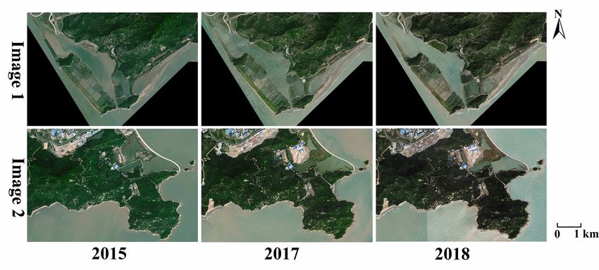
ISPRS Int. J. Geo-Inf. 2021, 10, 451                                                                                             2 of 17

                                       the extraction demands. On the other hand, it is no longer a problem to obtain high-
                                       resolution images such as WorldView-2 (WV-2) with the development of aerospace remote
                                       sensing technology [7,8], which guarantees the effective resolution of the data source.
                                       After comprehensive consideration, it is significant to propose a method for tidal flat
                                       wetland extraction from high-resolution images [9].
                                             Although there are no specific remote sensing methodologies for tidal flat wetland
                                       extraction, numerous extraction methods have been applied to convert remote sensing data
                                       into other land cover maps. A general method comprises combining mathematical statistics
                                       with manual interpretation. However, it is inefficient, with low accuracy, intensive labor,
                                       and dependence on human analysis. Multiple intelligent methods have been recommended
                                       in image extraction, such as multisource information fusion technology used in remote
                                       sensing mapping. Synthesis of spectral features [10,11] can distinguish targets by different
                                       brightness levels between image bands, classification by the fusion of different texture
                                       information [12] can take both the macroscopic nature and the detailed structure of targets
                                       into account, normalized difference index information [13,14] contributes to eliminating the
                                       influence of the difference in topography, and the combination of expert knowledge [15]
                                       is conducive to comprehensive interpretation and decision analysis of remote sensing
                                       images. The composition technology of multisource information has achieved specific
                                       results; however, depending on multisource information exclusively is not enough to
                                       extract the research targets accurately. Therefore, the proposed method is a combination of
                                       multisource information composition and multiclassification technologies.
                                             Traditional remote sensing image classification technology has been divided into un-
                                       supervised classification and supervised classification [16]. In unsupervised classification,
                                       statistical distance is typically used to measure the similarity, and the category intervals are
                                       maximized by distinguishing targets based on a specific algorithm [17,18]. When a specific
                                       set of targets is desired, supervised classification is more appropriate. The sample set of
                                       each category is selected first, a classification algorithm can be trained using the samples,
                                       and, finally, the remaining pixels are classified. The maximum likelihood classification
                                       (MLC) [19,20] method is a generally used supervised classification algorithm that estab-
                                       lishes a nonlinear discriminant function set according to the Bayesian information criterion
                                       (BIC) [21]. The support vector machine (SVM) [22–24] method is a widely used classifica-
                                       tion method in remote sensing images based on the structural risk minimization principle.
                                       The decision tree (DT) [25,26] algorithm is also a supervised classification method based on
                                       spatial data mining and knowledge discovery. Prior knowledge can be used in supervised
                                       classification to select training samples, and the classification accuracies can be improved by
                                       repeatedly testing training samples. However, supervised classification methods depend
                                       on the quality of training samples excessively, which makes it inefficient to select samples
                                       with more human capital and time. Moreover, supervised classification can only identify
                                       specific categories, which is not conducive to the classification of complex targets.
                                             In recent years, deep learning [27] methods have also been employed in the research
                                       of remote sensing information extraction. An algorithm named deep belief network
                                       (DBN) [28] has unleashed the characteristics of unsupervised learning with the identifica-
                                       tion of remote sensing features. However, the selection of network parameters requires
                                       the intervention of prior knowledge, which makes it difficult to determine the appropriate
                                       parameters. The generally used convolutional neural network (CNN) [29,30] algorithm in
                                       the deep learning method has obvious advantages in processing high-dimensional images,
                                       but the scanty samples of remote sensing images have limited the generalization ability
                                       of the CNN algorithm. Another deep learning algorithm, autoencoder (AE) [31,32], still
                                       needs to be combined with other classifiers to achieve appropriate results. Compared
                                       with traditional machine learning methods, deep learning methods have stronger fitting
                                       capabilities, and they can learn beneficial features from numerous data. However, they
                                       similarly rely on training samples excessively. Researchers have to spend a lot of time
                                       and energy collecting appropriate samples. Additionally, deep learning methods require
                                       high-performance computers to achieve fast computing and have time-consuming training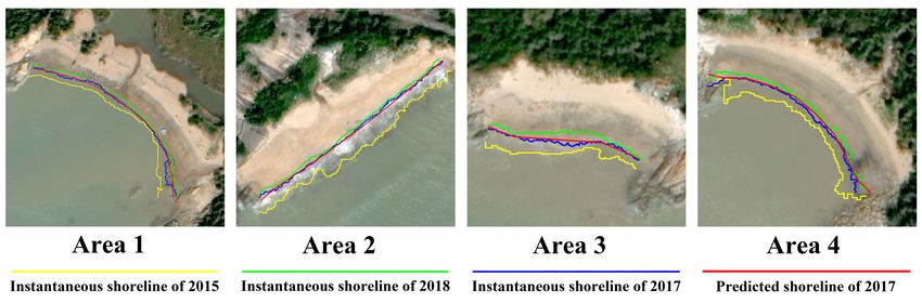
ISPRS Int. J. Geo-Inf. 2021, 10, 451                                                                                           3 of 17

                                       procedures, so they are not suitable for the extraction of small targets with limited samples
                                       such as shore targets. Therefore, it is necessary to design a comprehensive and complete
                                       extraction method for shores considering the inadequacy of existing methods.
                                             The aim of this study is to propose a method specifically for tidal flat wetland de-
                                       lineation and classification from high-resolution images and evaluate the method. First,
                                       remote sensing features and geographical buffers are used to establish a decision tree for
                                       initial classification. Next, a natural shoreline prediction algorithm is designed to refine
                                       the range of the tidal flat wetland. Then, a range and standard deviation descriptor is con-
                                       structed to extract the rock marine shore, a category of tidal flat wetlands. A geographical
                                       analysis method is considered to distinguish the other two categories of tidal flat wetlands.
                                       Finally, a tidal correction strategy is used to regulate the borderline of tidal flat wetlands
                                       to conform to the actual situation. The performance of each step is evaluated, and the
                                       results of this method were compared with existing available methods to illustrate the
                                       effectiveness and practicability of the proposed method. As a first application, this method
                                       is demonstrated in Hengqin Island (an island in China facing directly to the South China
                                       Sea). A better understanding of the distribution of shores in Hengqin Island is critical to
                                       wetland protection and construction planning.

                                       2. Methods
                                       2.1. Overall Processes
                                            The proposed method originates from the perspective of logical layering. According
                                       to the definition of tidal flat wetlands, it belongs to natural wetlands, and there are three
                                       categories, including rocky marine shore (RMS), mud marine shore (MMS), and sand
                                       marine shore (SMS). On the first logical level, the approximate range of the tidal flat
                                       wetland was extracted, which is regarded as the initial classification. Then, the range was
                                       refined on the second logical level by predicting the natural shore edges. Finally, the target
                                       objects were reclassified on the third logical level to obtain the three wetland categories.
                                       The classification system and the logical structure are shown in Figure 1. The overall
                                       flowchart is shown in Figure 2, and the procedures are summarized as follows.

                                                   Figure 1. Logical structure of this study.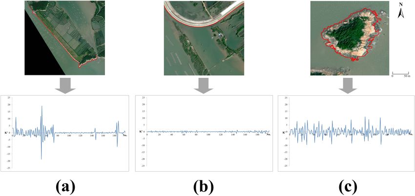
ISPRS Int. J. Geo-Inf. 2021, 10, 451                                                                                                        4 of 17

                                       Figure 2. Overall flowchart of the proposed method.

                                       2.1.1. Preprocessing
                                             Radiation calibration, geometric correction, data fusion, and segmentation are in-
                                       cluded in this step. In order to minimize the local differences of image objects and make
                                       the remote sensing features of each category prominent, multiresolution segmentation
                                       achieved by the fractal net evolution approach (FNEA) was conducted on the research
                                       images before classification via the software eCognition Developer 9.0. After repeated
                                       experiments, three segmentation parameters of FNEA were arranged: the scale parameter
                                       was 200, the shape index was 0.1, and the compactness was 0.5. The categories involved in
                                       this study could be distinguished optimally with the parameters above.

                                       2.1.2. Initial Classification
                                            The purpose of this step is to perform initial classification on the high-resolution
                                       images to extract the shore area roughly, i.e., accomplish Logic Layer 1 in Figure 1. There
                                       is both water and vegetation in the targets to be classified; therefore, it is important for
                                       the remote sensing features to be sensitive to water and vegetation. Normalized difference
                                       indexes are often used in the classification of remote sensing images because they are
                                       easy to compare, for which reason we chose the commonly used NDWI and NDVI to
                                       distinguish water and vegetation. Considering the adjacent distance between shore and
                                       sea, we divided the water into seawater and non-seawater according to the acreage of water
                                       targets, and the buffer zone of seawater targets was constructed to restrict the distribution
                                       of targets. The features explored in this study and their descriptions are shown in Table 1.

                                       Table 1. Summary of the features explored in this study and their descriptions.

                                       Name                                                              Description
                                       NDWI                                           (RGREEN-RNIR)/(RGREEN + RNIR) [33]
                                       NDVI                                              (RNIR-RRED)/(RNIR + RRED) [34]
                                       Area                                 Pixel numbers of target object multiply area of every single pixel
                                       Buffer                                      Whether the target object is within the buffer area
                                       where RGREEN, RNIR, and RRED are the reflectance values in the green (Band 2), NIR (Band 4) and red (Band 3)
                                       bands, respectively.

                                            First, we sampled the categories to be classified, and then we calculated the NDWI
                                       of each sample. In this study, the sample number of each category is 200, and the NDWI
ISPRS Int. J. Geo-Inf. 2021, 10, 451                                                                                          5 of 17

                                       value lines are shown in Figure 3a. TW represents the optimal threshold, which maximizes
                                       the distinction between water and nonwater. It can be observed that water and nonwater
                                       objects can be distinguished when TW ranges from 0 to 0.5. To obtain the specific value,
                                       we calculated the classification deviations (the total deviation of the misclassified samples
                                       in the target category and the nearest nontarget category) in this range, as shown in
                                       Figure 3b. The minimum deviation exists when the NDWI equals 0.11. Similarly, TV
                                       represents the optimal threshold, which maximizes the distinction between vegetation and
                                       nonvegetation objects, and the value of TV can be determined as 0.65, as shown in Figure 4.
                                       In addition, Smax represents the merged water object with the largest area. The decision
                                       tree was established, as shown in Figure 5, and the classification was executed based on
                                       the rules. In order to improve the initial classification results, it was necessary to merge
                                       the connected objects and remove the small patches. Then, the rough scope of shore areas
                                       could be obtained.

      Figure 3. Determination of Tw . (a) NDWI line of each category. (b) Deviation trend with the NDWI value changing
      from 0 to 0.5.

      Figure 4. Determination of Tv . (a) NDVI line of each category. (b) Deviation trend with the NDVI value changing
      from 0.4 to 0.7.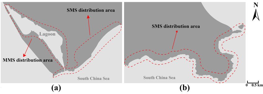
ISPRS Int. J. Geo-Inf. 2021, 10, 451                                                                                            6 of 17

                                       Figure 5. Decision tree for the initial classification.

                                       2.1.3. Classification Refinement
                                             The purpose of this step is to refine the range of tidal flat wetlands. The rough scopes
                                       of shore areas obtained in the initial classification contained both natural boundaries and
                                       artificial ones, while the latter did not belong to tidal flat wetlands. To predict the natural
                                       boundaries to refine the tidal flat wetlands, an algorithm based on the slope change of
                                       target edges was designed and is explained in Section 2.2 in detail.

                                       2.1.4. Reclassification
                                             In this step, reclassification was conducted to extract the RMS, MMS, and SMS. First,
                                       a new feature descriptor based on the range and standard deviation was designed to
                                       extract the RMS. Then, a geographical analysis method was utilized to classify the MMS
                                       and SMS. Finally, a tidal correction method was applied to predict the low tide beach line
                                       of tidal flat wetlands in order to obtain the complete wetland targets. The range/standard
                                       deviation description method and the tidal correction method will be described in detail
                                       from Sections 2.3 to 2.4. The geographical analysis method applied to distinguish the MMS
                                       and SMS will be explained in this section.
                                             The composition of the SMS is similar to the MMS, and their slight differences lie in the
                                       sizes of sand or mud particles, which are usually distinguished by manual exertion. Limited
                                       by resolution, it is still a problem to distinguish them by remote sensing features, even
                                       in high-resolution images. Fortunately, the SMS and MMS have obvious discriminations
                                       according to their causes and distributions. The SMS is generally formed of stones being
                                       sharpened into small particles by waves, so they are mostly distributed in the shore areas
                                       directly towards the ocean with strong wave effects. The MMS is formed by sediments
                                       of mud. They are distributed in areas with slow currents and weak wave effects, such
                                       as lagoons and estuaries. Therefore, the geographical analysis method is proposed to
                                       distinguish the SMS and MMS.
                                             Hengqin Island, to which the study area belongs, is an island towards lands from
                                       the north, west, and east sides, but only the south side points directly towards the South
                                       China Sea. In Image 1, the SMS and MMS are distributed around an obvious lagoon and
                                       the south shore area with strong wave effects. According to the geographical causes and
                                       definitions above, we could scope the distribution range of the two shore wetlands. The
                                       SMS was distributed around the lagoon, and the MMS was distributed in the south shore
                                       area. As a result, the shore wetlands were distinguished, as shown in Figure 6a. In Image 2,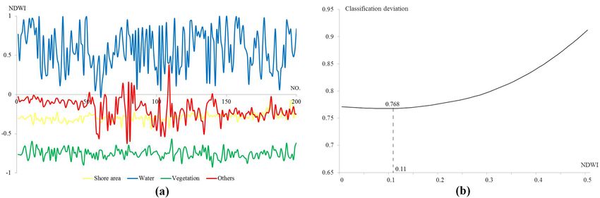
ISPRS Int. J. Geo-Inf. 2021, 10, 451                                                                                             7 of 17

                                       natural shores are all distributed in the south areas towards the ocean, which means there
                                       are no appropriate circumstances for the MMS. Therefore, the natural shores in Image 2
                                       were all classified into SMS instead of RMS, as shown in Figure 6b.

      Figure 6. The geographical analysis method used to distinguish the SMS and MMS. (a) Geographical analysis in Image 1.
      (b) Geographical analysis in Image 2.

                                       2.2. Natural Shoreline Prediction
                                            Artificial shorelines are often difficult to distinguish from natural ones because of their
                                       similar spectral or texture features. Considering that edges of artificial shores are usually
                                       regular and the natural shores are not, a natural shoreline prediction (NSP) algorithm based
                                       on the slope change rate of edges was designed.
                                            For the rough shore area extracted in the initial classification, the shore polygon edge
                                       adjacent to the sea water was defined as a line vector named L, and L was equally divided
                                       into n sections from l1 to ln . Then, the slope of each l as Ki was calculated

                                                                                       ye − ys
                                                                                Ki =                                                 (1)
                                                                                       xe − xs

                                       where ( xs , ys ) and ( xe , ye ) represent the start point and the end point of each section,
                                       respectively.
                                             The serial number of l is selected as the abscissa, and the slope of l is selected as the
                                       ordinate to obtain a slope change curve y = f (k). The change rate of Ki as Ki0 was calculated,
                                       after which the slope change rate curve could be obtained. In order to distinguish the stable
                                       section and the fluctuation section of the curve, a threshold T was set (T, defined as one-
                                       twentieth of the difference between the max and the minimal Ki0 ), and when Ki0 ∈    / [− T, T ],
                                       l was predicted as a natural shoreline. The steps of the proposed NSP algorithm are
                                       summarized in Algorithm 1.

                                         Algorithm 1: Natural Shoreline Prediction.
                                           1. Define the shore polygon edge as a line vector L.
                                           2. Divide L equally into n sections from l1 to ln .
                                           3. Calculate the slope of each l as Ki , and obtain the slope change curve.
                                           4. Calculate the change rate of Ki as Ki0 , and obtain the slope change rate curve.
                                           5. Set a threshold T and when Ki0 ∈ / [− T, T ], l is predicted as a natural shoreline.

                                       2.3. Range and Standard Deviation Description
                                            In order to minimize the difference of image objects, the previous steps were based
                                       on object-oriented segmentation. However, there were two problems. On the one hand,
                                       the rock targets had different particle sizes compared to the other two targets, which
                                       means they had different textural features, and it was hard to keep the texture differences
                                       on the same scale. In this way, appropriate segmentation scales to preserve the textural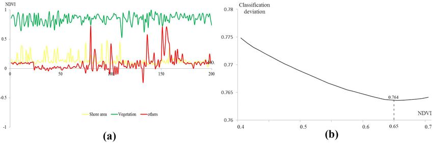
ISPRS Int. J. Geo-Inf. 2021, 10, 451                                                                                                8 of 17

                                       features of both the RMS and other targets were difficult to select. On the other hand,
                                       the spectral features of the RMS, SMS, and MMS were similar, which made it troublesome
                                       to distinguish any of them, even at an object-oriented level. Considering the problems
                                       above, a pixel-based extraction method was designed and is presented in this part.
                                            Observing the characteristics of the three shore wetlands, we found that the RMS has
                                       a more complex texture than the others, resulting in discrete gray values in a window with
                                       a certain scale. Hence, the range and standard deviation, which reflect the tightness and
                                       dispersion of the data, were selected to design a new feature description—the range and
                                       standard deviation (RSD) descriptor. Despite that high-resolution images with four bands
                                       contain plenty of information, the quantity of redundant information exists when they
                                       are employed to extract the RMS, as shown in Figure 7a. Therefore, two bands with less
                                       relevance were selected for feature description, as shown in Figure 7b. The specific steps of
                                       this method are described as follows.
                                       (1)   Clip the high-resolution images by polygons of the refined tidal flat wetlands, and
                                             reserve the blue band and the near-infrared band.
                                       (2)   Traverse each band by a window of 5 × 5, and calculate the standard deviation of
                                             each window as σ and the range of each window as R. Then, assign the standard
                                             deviation and range value to all pixels in the window so that we can get four dispersion
                                             measurement images.

      Figure 7. Band selection of high-resolution images. (a) The image consists of four bands (blue, green, red, and near infrared).
      The RMS has mixed spectral features with the other two types and quantities of redundant information that exist. (b) Little
      redundant information exists when there are only two bands left (blue and near infrared), which means less complexity and
      calculations of the algorithm.

                                            It is worth mentioning that the 5 × 5 window in this step is the optimal traversal
                                       window selected by repeated experiments. The experimental results of the other windows
                                       are shown in Figure 8 and Table 2.

                                       Table 2. Extraction accuracies of the RMS when using windows with different sizes.

                                        Size               3×3               4×4               5×5               6×6                7×7

                                       OA (%)              77.04             80.22             83.53             80.37              80.90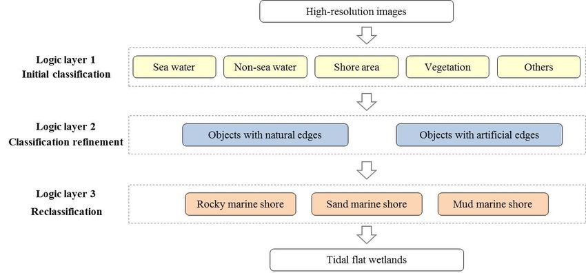
ISPRS Int. J. Geo-Inf. 2021, 10, 451                                                                                             9 of 17

                                       Figure 8. Extraction results of the RMS when using windows with different sizes.

                                       (3)   The four images were added together by influence weights to obtain the final measures
                                             of the dispersion image. In order to evaluate the contribution of each dispersion
                                             measurement image, the information entropy was estimated as

                                                                                    255
                                                                               E=   ∑ pi logpi                                      (2)
                                                                                    i =0

                                             where pi is the probability of gray value i.
                                             Then, the weights were calculated as

                                                                                          Ek
                                                                               Wk =     4
                                                                                                    .                               (3)
                                                                                      ∑ k =1   Ek

                                       (4)   The Marr edge detection operator was used in the final measures of the dispersion
                                             image to determine the RMS edge so that the RMS was extracted.

                                       2.4. Tidal Correction
                                            Influenced by tidal actions, tidal flat wetlands emerge differently in images at different
                                       moments of the same day. Thus, it was necessary to determine the low tide location for
                                       a more accurate extraction of tidal flat wetlands in actual demands. In order to predict
                                       the low tidal flat line of tidal flat wetlands, the slope of the tidal flat was calculated first
                                       according to the tidal height difference and the instant waterlines of one place at a different
                                       time. Then, the low tidal flat line of the wetlands was corrected to the low tide line.
                                            The principle of tidal correction is shown in Figure 9, and the implication of each
                                       character is explained below the figure. By computing the tidal height difference between
                                       different time and the average distance of the instantaneous waterlines of two phases, the
                                       angle of the tidal flat slope θ is calculated as

                                                                                            ∆H
                                                                               θ = arctan      .                                    (4)
                                                                                            ∆L
                                            According to the average low tide height Hlow , the correction distance Llow , i.e., the
                                       low tide line is computed as
                                                                                  h − Hlow
                                                                          Llow =                                                  (5)
                                                                                    tanθ
ISPRS Int. J. Geo-Inf. 2021, 10, 451 10 of 17
where h represents the tide height in the satellite transit time. After tidal correction, the
results of the complete tidal flat wetlands could be obtained.
Figure 9. Schematic diagram of tidal correction. θ is the angle of the tidal flat slope. H1 and H2
represent the tide height at Time 1 and Time 2, respectively. ∆H is the tidal height difference between
different times, and ∆L represents the average distance of the instantaneous waterlines of the two
phases. Hlow is the average low tide height.
The tidal correction method is based on the assumption that the tidal flat slope is a
gentle slope formed under the action of waves. The bottom matrix of the rocky coast is rel-
atively hard, and the muddy beaches are mostly distributed around the lagoon. Therefore,
these two types of tidal flat wetlands are less affected by the waves. The boundary of the
low tide beach is to extract the water edge, so the tide level correction method in this study
was mainly applied to the low tide beach boundary correction of sandy beaches. The key to
the effectiveness of this method is whether the tidal flat slope is a gentle slope with a stable
slope. In order to verify the correctness of this hypothesis, we first calculated the slope
angle of the tidal flat based on the above principle, and then we obtained a high-resolution
image of the third time phase of the same area and calculated the instantaneous waterline
of that phase based on the slope angle and the imaging time of the third time phase image.
We compared the actual extracted instantaneous water edge. If the two were similar, it
indicated that the tidal flat slope angle remained unchanged; that is, the tide level correction
method was effective.
To specifically evaluate the performance of tidal correction, the tidal flat slope was
first calculated according to the information from Time 1 and Time 2. Then, the predicting
instant waterline of the third time could be obtained on the basis of the tidal flat slope and
the instant tide height, while the actual instant waterline could be acquired from the three
previous extraction steps. Then, m sample points were chosen from the predicting instant
waterline and the actual one. The root mean square error (RMSE), the mean absolute error
(MAE), and the standard deviation (SD) between the two waterlines were calculated to
evaluate their deviation quantitatively, expressed as
s
m
1
RMSE =
m ∑ di 2 (6)
i =1
m
1
MAE =
m ∑ di (7)
i =1
s
m
1
SD =
m ∑ ( d i − d u )2 (8)
i =1
where m represents the number of sample points, di represents the Euclidean distance of
point i between two lines, and du is the average value of di .ISPRS Int. J. Geo-Inf. 2021, 10, 451 11 of 17
3. Results and Discussions
3.1. Research Data
Six WorldView-2 images (Figure 10), located in Hengqin Island, Guangdong Province,
China, respectively, acquired on 21 October 2015, 1 November 2017, and 15 January 2018,
were utilized in this study. The Gram–Schmidt spectral sharpening method was used to
fuse the multispectral bands and the panchromatic band, and then the cubic convolution
method was used to resample the fusion images to an identical resolution. Detailed
parameters of the used data are described in Table 3. Fusion images were finally used,
containing red, green, blue, and near-infrared bands with a resolution of 0.5 m. The sizes
of Image 1 and Image 2 are 11, 176 × 7466 and 7446 × 5631 pixels, respectively.
Table 3. Detailed parameters of the used data.
Name Parameters
Satellite WorldView-2 (including multispectral and panchromatic sensors)
The regression period 1.1 days
450–1040 (panchromatic), 450–510 (blue), 510–580 (green),
Wavelength (nm)
630–690 (red), and 770–895 (NIR)
Original resolutions 2015.10.21 — 1.891 (multispectral) and 0.473 (panchromatic)
Spatial resolution (nm) 2017.11.01 — 1.321 (multispectral) and 0.330 (panchromatic)
2018.01.15 — 1.332 (multispectral) and 0.333 (panchromatic)
Fusion method Gram–Schmidt spectral sharpening method
Resampling method Cubic convolution method
Figure 10. Research images from three years.
3.2. Performance of NSP
According to the NSP algorithm, slope change rate curves of different shore polygon
edges were calculated, and the results are shown in Figure 11. There is a shoreline with
both natural features and artificial features in the test area in Figure 11a. It can be seen from
the slope change rate curve that the slope fluctuates at the beginning and then becomes
steady from a certain point. According to the different fluctuant characteristics of the slope
change rates, it is clear that the left part of the curve comes from the natural excerpt, and
the right part comes from the artificial one. Figure 11b,c demonstrates the slope change rate
curve of an artificial shoreline and a natural shoreline, which express the same fluctuations
as in Figure 11a.ISPRS Int. J. Geo-Inf. 2021, 10, 451 12 of 17
Figure 11. Examples of slope change rate curves from different shore polygon edges. (a) Slope change rate curves of the
area with both the artificial shore and the natural shore. (b) Slope change rate curves of the artificial shore. (c) Slope change
rate curves of the natural shore.
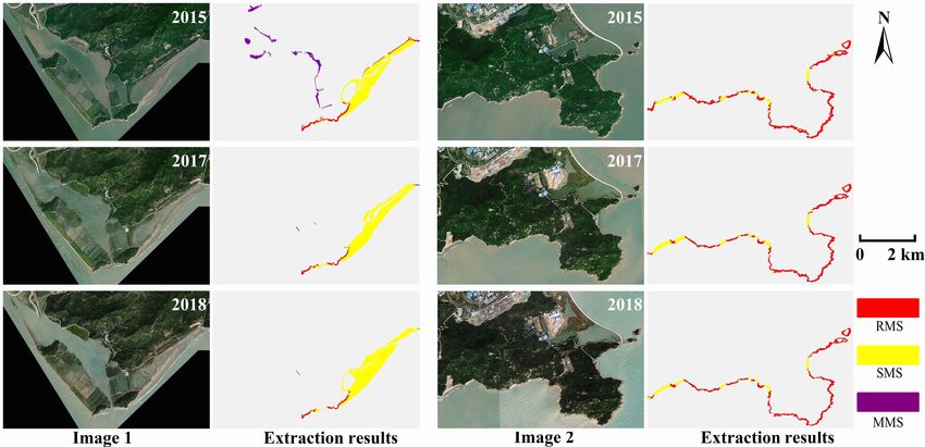
The NSP algorithm was executed on two images from 2015. The results are shown
in Figure 12, and the evaluating data are listed in Table 4. When the extraction results of
Image 1 were compared with the ground truth, it can be seen from Figure 12a that most of
the natural shores were extracted correctly, with only a small number of misextractions
around the shore edges. Extraction accuracies and the kappa coefficient in Table 4 justify
the analysis above. The extraction results of Image 2 in Figure 12b are approximately
correct, with a producer’s accuracy of 88.00% and a user’s accuracy of 93.53%. However,
it can be seen from Figure 12a that an unnatural shore on the far north side of Image 1
was mistakenly extracted as a natural shore due to its irregular edge. In Image 2, there are
also some misextractions at the junction of the two shore types on the middle east side.
The misextractions illustrate the limitations of the NSP algorithm in that it is excessively
dependent on the shape of shore edges. In this condition, manual corrections will be needed
according to practical applications. Despite some defects in these particular situations, the
algorithm in this step performed well in the general prediction of natural shorelines.
Table 4. Extraction accuracies and the kappa coefficient after NSP.
PA (%) UA (%) OA (%) κ
Image1 94.25 89.70 99.64 0.9161
Image2 88.00 93.53 99.41 0.9050
Figure 12. Results after NSP from two images in 2015. (a) Groundtruth and result of Image 1. (b) Groundtruth and result of
Image 2.ISPRS Int. J. Geo-Inf. 2021, 10, 451 13 of 17
3.3. Effectiveness of Tidal Correction
In this study, images from 2015 and 2018 were, respectively, selected as the first
and second time to calculate the tide flat slope, and images from 2017 were selected for
evaluation. According to the method in Section 2.4, the instant waterline prediction results
of the four typical experimental areas are illustrated in Figure 13, and the corresponding
accuracy indexes are shown in Table 5.
Figure 13. Tidal correction of four typical experimental areas.
In Figure 13, blue lines represent the actual extracted instant waterlines, and red lines
represent the predicted ones according to the tidal correction method. In Area 1, most of
the actual waterline and the predicted waterline coincide, but only small sections around
the right endpoint deviate from each other. Observed from the image, we can see that there
are rocks located in the sand marine shore, which could have prevented the sand shore
from forming a gentle slope. Therefore, the terrain of the right shore does not conform to
the hypothetical topography, resulting in a mistake. As shown in Area 2, Area 3, and Area
4, the real waterlines coincide well with the predicted ones, and the accuracy indexes in
Table 5 also confirm the consequent RMSE and MAE of less than 2 and the SD less than
0.6, which verifies the performance of the tidal correction. When the tidal correction is
conducted, each nonadjacent tidal flat wetland has to be processed independently, which
means that low efficiency could be a defect of this method. Thus, we may consider parallel
processing in future attempts.
Table 5. Tidal correction evaluation results.
RMSE MAE SD
Area 1 1.98 1.70 2.41
Area 2 1.08 0.97 0.38
Area 3 1.28 1.14 0.58
Area 4 1.88 1.81 0.58
3.4. Comparison with Other Methods
In this section, the proposed method is applied to six experimental images from three
years, and Figure 14 presents the results. It can be seen that the proposed method is able to
delineate and classify most of the tidal flat wetlands and provide satisfactory results.
In order to fully verify the advantages of the proposed method, both classical machine
learning methods and deep learning methods were considered as comparison methods.
In terms of classical machine learning methods, no methods were specifically used for tidal
flat wetland extraction; therefore, the support vector machine (SVM) method [24] and the
random forest (RF) method [35], which performed better than the others in the situation
of this research through experiments, were selected as comparison methods. In terms
of deep learning methods, considering the suitable classification methods and the hashISPRS Int. J. Geo-Inf. 2021, 10, 451 14 of 17
rate of our computers comprehensively, the ResNet34 model [36] was selected as the third
comparison method.
Figure 14. Tidal flat wetlands extraction results of the proposed method.
In order to guarantee the same training samples, FNEA segmentation was conducted
on the research images from October 21, 2015, at first, sharing the same parameters of FNEA
with the proposed method (detailed values are clarified in Section 2.1.1). Samples of each
tidal flat wetland category (in the form of objects) were obtained by manual interpretation
and treated as the training samples of ResNet34. Then, the object-based samples were
transformed into pixel-based ones, which were considered as the training samples of
the SVM and RF. Finally, 63 objects in Image 1 and 77 objects in Image 2 were selected
as training samples. Moreover, all the comparison methods were conducted from the
perspective of logical layering (the same initial classification and geographical analysis),
which guaranteed a fair comparison. To quantify the performance values, the overall
accuracy (OA) and kappa (k) were selected to evaluate the four methods. There are 400
and 350 verification points in Image 1 and Image 2, respectively, for the experimental data
from each year.
Figure 15a–f provides a visual comparison of the different methods, and the corre-
sponding statistical results are listed in Table 6. For the SVM method, land and sea are
separated in Image 1 from all three years, which mainly depends on the results of the initial
classification in this study. There are still misclassifications when observing the details: the
RMS and the SMS on the south coast are not distinguished, the RMS and the MMS around
the lagoon are mixed, and the white waves in the sea are also misclassified into tidal flat
wetlands due to their similar spectral features. The results of the SVM in Image 2 are a
little more reliable than those in Image 1 when noticing the OA, which are caused by fewer
tidal flat wetland categories, but it still shows a large number of misclassifications from the
visual results. Moreover, the SVM method cannot distinguish between the artificial bound-
aries and the natural boundaries; for example, the artificial roads in the northeast corner
of Image 2 are misclassified as natural targets. The extraction results of the RF method
contain too much “salt-and-pepper noise" just as the SVM, despite the fact that it performs
better than the SVM in accuracies, which are caused by their pixel-based classification
modus. The ResNet34 model is conducted in an object-based way, just as the proposed one,
which can solve the noise problems. Observing the visual results, we can clearly notice
that the last two object-based methods perform well in achieving the purity of results.
For ResNet34, there are also misclassifications between artificial boundaries and natural
boundaries: the artificial roads in the northwest corner and the artificial coast on the westISPRS Int. J. Geo-Inf. 2021, 10, 451 15 of 17
are mistaken for tidal flat wetlands in Image 1 from all three years. Additionally, ResNet34
performs poorly when distinguishing the RMS from the other two kinds. Large sample
quantity reliance is the main limitation of deep learning methods, although there are only
a small number of samples in this study that caused unsatisfying results when ResNet34
was unable to learn enough features of tidal flat wetlands. It can be concluded that the
ResNet34 model has limitations when extracting tidal flat wetlands from high-resolution
images when there are not enough samples. With the same samples, the proposed method
performs well when solving misclassification problems, which can be seen from the results.
The proposed NSP algorithm distinguishes the misclassifications of artificial objects from
natural objects, and the RSD feature descriptor can easily extract the RMS when it has
similar spectral characteristics with the surroundings. It can be seen from Table 6 that the
OA of the proposed method are all above 88%, exceeding the three compared methods.
Concluding the comparison results, the pixel-based SVM and RF methods cause “salt-
and-pepper noise” and misclassifications when extracting tidal flat wetlands. The deep
learning model solves the noise problem, while it still shows unsatisfying results with
insufficient samples. The proposed method performs well in these aspects despite its
lower processing speed. Additionally, there is no other efficient method with similar
accuracy to the proposed one, which means an excellent extraction consequence is more
significant, despite the fact that there are complex steps in the proposed method. Therefore,
the proposed method has particular advantages in the extraction of tidal flat wetlands from
high-resolution images.
Figure 15. Comparison of results with other methods: (a) results of Image 1 in 2015; (b) results of Image 2 in 2015; (c) results
of Image 1 in 2017; (d) results of Image 2 in 2017; (e) results of Image 1 in 2018; (f) results of Image 2 in 2018.ISPRS Int. J. Geo-Inf. 2021, 10, 451 16 of 17
Table 6. Comparison of the accuracy of the four wetland classification methods.
SVM RF ResNet Proposed
Time OA (%) κ OA (%) κ OA (%) κ OA (%) κ
2015 51.25 0.34 66.50 0.51 53.25 0.37 88.50 0.84
Image 1 2017 53.00 0.10 69.25 0.46 75.00 0.46 92.75 0.84
2018 53.75 0.28 64.75 0.33 76.00 0.55 93.50 0.87
2015 71.43 0.49 44.86 0.24 57.71 0.37 96.29 0.93
Image 2 2017 72.29 0.52 63.14 0.44 57.43 0.35 95.71 0.92
2018 76.57 0.58 73.14 0.56 48.00 0.24 92.86 0.87
4. Conclusions
In this study, a comprehensive method for tidal flat wetland extraction from high-
resolution images was proposed. First, the decision tree method based on remote sensing
features and geographical buffers was constructed for the initial classification. Next, an NSP
algorithm based on the slope change rate was designed to refine the range of the tidal
flat wetland. Then, a range and standard deviation descriptor was constructed to extract
the RMS, and a geographical analysis method was considered to distinguish the SMS and
MMS. Finally, a tidal correction strategy was introduced to regulate the borderline of tidal
flat wetlands. The results showed that the proposed method can achieve good performance
for the extraction of tidal flat wetlands from high-resolution images. By the delineation
and classification method, the distribution of tidal flat wetlands can be investigated easily,
consequently contributing to wetland protection.
A defect still comes from the strong correlation between the multiple steps, which
means that the results of the previous step will affect the results of the following step
directly. Therefore, emphasis will be placed on optimizing the accuracy in each step in the
future. In addition, we will try to expand this method to more complex shore situations in
order to increase the versatility.
Author Contributions: Conceptualization, Hong Pan and Yonghong Jia; Data curation, Hong Pan,
Dawei Zhao, Tianyu Xiu and Fuzhi Duan; Formal analysis, Hong Pan; Investigation, Hong Pan,
Dawei Zhao, Tianyu Xiu and Fuzhi Duan; Methodology, Hong Pan; Supervision, Yonghong Jia;
Validation, Hong Pan; Writing—original draft, Hong Pan; Writing—review and editing, Hong Pan
and Yonghong Jia. All authors have read and agreed to the published version of the manuscript.
Funding: This research was funded by Development Fund of the National Surveying and Mapping
Science and Technology.
Institutional Review Board Statement: Not applicable.
Informed Consent Statement: Not applicable.
Data Availability Statement: Data or models support the findings of this study are available from
the corresponding author upon reasonable request.
Conflicts of Interest: The authors declare no conflict of interest.
References
1. Batzer, D.P. Wetland ecology: Principles and conservation. Wilson Bull. 2001, 113, 354–361. [CrossRef]
2. Cahoon, D.R.; Hensel, P.F.; Spencer, T.; Reed, D.J.; Saintilan, N. Coastal Wetland Vulnerability to Relative Sea-Level Rise: Wetland
Elevation Trends and Process Controls. In Wetlands and Natural Resource Management; Springer: Berlin/Heidelberg, Germany, 2006.
3. Bellio, M.; Kingsford, R.T. Alteration of wetland hydrology in coastal lagoons: Implications for shorebird conservation and
wetland restoration at a Ramsar site in Sri Lanka. Biol. Conserv. 2013, 167, 57–68. [CrossRef]
4. David, M.M.; Meli, P.; Maria, I.V.R.; Aronson, J. Ecosystem response to interventions: Lessons from restored and created wetland
ecosystems. J. Appl. Ecol. 2015, 52, 1528–1537.
5. Klemas, V. Remote Sensing of Riparian and Wetland Buffers: An Overview. J. Coast. Res. 2014, 297, 869–880. [CrossRef]
6. Kuklinski, P. Ecology of stone-encrusting organisms in the Greenland Sea—A review. Polar Res. 2009, 28, 222–237. [CrossRef]
7. Ghosh, A.; Joshi, P.K. Assessment of pan-sharpened very high-resolution WorldView-2 images. Int. J. Remote Sens. 2013, 34,
8336–8359. [CrossRef]ISPRS Int. J. Geo-Inf. 2021, 10, 451 17 of 17
8. Pu, R.; Landry, S. A comparative analysis of high spatial resolution IKONOS and WorldView-2 imagery for mapping urban tree
species. Remote Sens. Environ. 2012, 124, 516–533. [CrossRef]
9. Carle, M.V.; Wang, L.; Sasser, C.E. Mapping freshwater marsh species distributions using WorldView-2 high-resolution multispec-
tral satellite imagery. Int. J. Remote Sens. 2014, 35, 4698–4716. [CrossRef]
10. Li, H.; Wang, Y.; Xiang, S.; Duan, J.; Zhu, F.; Pan, C.; Com, H. A label propagation method using spatial-spectral consistency for
hyperspectral image classification. Int. J. Remote Sens. 2016, 37, 191–211. [CrossRef]
11. Lahet, F.; Ouillon, S.; Forget, P. Colour classification of coastal waters of the Ebro river plume from spectral reflectances. Int. J.
Remote Sens. 2001, 22, 1639–1664. [CrossRef]
12. Kong, D.; Xu, J.; Yin, J.; Yan, H. Classification of MODIS images combining surface temperature and texture features using the
Support Vector Machine method for estimation of the extent of sea ice in the frozen Bohai Bay, China. Int. J. Remote Sens. 2015, 36,
2734–2750.
13. Defries, R.S.; Townshend, J.R.G. NDVI-derived land cover classifications at a global scale. Int. J. Remote Sens. 1994, 15, 3567–3586.
[CrossRef]
14. Wu, J.; Liu, Y.; Wang, J.; Ting, H. Application of Hyperion data to land degradation mapping in the Hengshan region of China.
Int. J. Remote Sens. 2010, 31, 5145–5161. [CrossRef]
15. Benferhat, S.; Boudjelida, A.; Tabia, K.; Drias, H. An intrusion detection and alert correlation approach based on revising
probabilistic classifiers using expert knowledge. Appl. Intell. 2013, 38, 520–540. [CrossRef]
16. Muchoney, D.; Borak, J.; Chi, H.; Friedl, M.; Gopal, S.; Hodges, J.; Morrow, N.; Strahler, A. Application of the MODIS global
supervised classification model to vegetation and land cover mapping of Central America. Int. J. Remote Sens. 2000, 21, 1115–1138.
[CrossRef]
17. Zhou, Y.; Xiao, X.; Qin, Y.; Dong, J.; Zhang, G.; Kou, W.; Jin, C.; Wang, J.; Li, X. Mapping paddy rice planting area in rice-wetland
coexistent areas through analysis of Landsat 8 OLI and MODIS images. Int. J. Appl. Earth Obs. Geoinf. 2016, 46, 1–12. [CrossRef]
18. Xiao, X.; Boles, S.; Liu, J.; Zhuang, D.; Frolking, S.; Li, C.; Salas, W.; Moore, I.B. Mapping paddy rice agriculture in southern China
using multi-temporal MODIS images. Remote Sens. Environ. 2005, 95, 480–492. [CrossRef]
19. Lyons, M.B.; Keith, D.A.; Phinn, S.R.; Mason, T.J.; Elith, J. A comparison of resampling methods for remote sensing classification
and accuracy assessment. Remote Sens. Environ. 2018, 208, 145–153. [CrossRef]
20. Raju, P.V. Classification of wheat crop with multi-temporal images: Performance of maximum likelihood and artificial neural
networks. Int. J. Remote Sens. 2003, 24, 4871–4890.
21. Carr, J.R. Spatial Statistics for Remote Sensing. Math. Geosci. 2005, 37, 549–550. [CrossRef]
22. Hearst, M.A.; Dumais, S.T.; Osman, E.; Platt, J.; Scholkopf, B. Support vector machines. IEEE Intell. Syst. 1998, 13, 18–28.
[CrossRef]
23. Yu, L.; Porwal, A.; Holden, E.J.; Dentith, M.C. Towards automatic lithological classification from remote sensing data using
support vector machines. Comput. Geosci. 2012, 45, 229–239. [CrossRef]
24. Maulik, U.; Chakraborty, D. A self-trained ensemble with semisupervised SVM: An application to pixel classification of remote
sensing imagery. Pattern Recognit. 2011, 44, 615–623. [CrossRef]
25. Friedl, M.A.; Brodley, C.E. Decision tree classification of land cover from remotely sensed data. Remote Sens. Environ. 1997, 61,
399–409. [CrossRef]
26. Pal, M.; Mather, P.M. An assessment of the effectiveness of decision tree methods for land cover classification. Remote Sens.
Environ. 2003, 86, 554–565. [CrossRef]
27. Hinton, G.E.; Osindero, S.; Teh, Y.W. A fast learning algorithm for deep belief nets. Neural Comput. 2017, 18, 1527–1554. [CrossRef]
28. Lin, L.; Dong, H.; Song, X. DBN-Based Classification of Spatial-Spectral Hyperspectral Data; Springer: Cham, Switzerland, 2017.
29. Qayyum, A.; Malik, A.S.; Saad, N.M.; Iqbal, M.; Abdullah, M.F.; Rasheed, W. Scene classification for aerial images based on CNN
using sparse coding technique. Int. J. Remote Sens. 2017, 38, 2662–2685. [CrossRef]
30. Shunping, J.; Chi, Z.; Anjian, X.; Yun, S.; Duan, Y. 3D Convolutional Neural Networks for Crop Classification with Multi-Temporal
Remote Sensing Images. Remote Sens. 2018, 10, 75.
31. Han, X.; Zhong, Y.; Zhao, B.; Zhang, L. Scene classification based on a hierarchical convolutional sparse auto-encoder for high
spatial resolution imagery. Int. J. Remote Sens. 2017, 38, 514–536. [CrossRef]
32. Othman, E.; Bazi, Y.; Alajlan, N.; Alhichri, H.; Melgani, F. Using convolutional features and a sparse autoencoder for land-use
scene classification. Int. J. Remote Sens. 2016, 37, 1977–1995. [CrossRef]
33. Gao, B. NDWI-a normalized difference water index for remote sensing of vegetation liquid water from space. Remote Sens.
Environ. 1996, 58, 257–266. [CrossRef]
34. Huete, A.; Didan, K.; Miura, T.; Rodriguez, E.P.; Gao, X.; Ferreira, L.G. Overview of the radiometric and biophysical performance
of the MODIS vegetation indices. Remote Sens. Environ. 2002, 83, 195–213. [CrossRef]
35. Breiman, L. Random forest. Mach. Learn. 2001, 45, 5–32. [CrossRef]
36. He, K.; Zhang, X.; Ren, S.; Jian, S. Deep Residual Learning for Image Recognition. In Proceedings of the 2016 IEEE Conference on
Computer Vision and Pattern Recognition (CVPR), Las Vegas, NV, USA, 27–30 June 2016; pp. 770–778.You can also read


