THE SPACENET MULTI-TEMPORAL URBAN DEVELOPMENT CHALLENGE
←
→
Page content transcription
If your browser does not render page correctly, please read the page content below
The SpaceNet Multi-Temporal Urban Development Challenge
                                                                      Adam Van Etten∗†                   Daniel Hogan∗

                                                                                           Abstract
arXiv:2102.11958v1 [cs.CV] 23 Feb 2021

                                                    Building footprints provide a useful proxy for a great many humanitarian applications. For
                                                example, building footprints are useful for high fidelity population estimates, and quantifying
                                                population statistics is fundamental to ∼ 1/4 of the United Nations Sustainable Development
                                                Goals Indicators. In this paper we (the SpaceNet Partners) discuss efforts to develop techniques
                                                for precise building footprint localization, tracking, and change detection via the SpaceNet
                                                Multi-Temporal Urban Development Challenge (also known as SpaceNet 7). In this NeurIPS
                                                2020 competition, participants were asked identify and track buildings in satellite imagery time
                                                series collected over rapidly urbanizing areas. The competition centered around a brand new
                                                open source dataset of Planet Labs satellite imagery mosaics at 4m resolution, which includes
                                                24 images (one per month) covering ≈ 100 unique geographies. Tracking individual buildings
                                                at this resolution is quite challenging, yet the winning participants demonstrated impressive
                                                performance with the newly developed SpaceNet Change and Object Tracking (SCOT) metric.
                                                This paper details the top-5 winning approaches, as well as analysis of results that yielded a
                                                handful of interesting anecdotes such as decreasing performance with latitude.

                                         1     Background
                                         Time series analysis of satellite imagery poses an interesting computer vision challenge with nu-
                                         merous human development applications. The SpaceNet 7 Challenge aims to advance this field
                                         through a data science competition aimed specifically at improving these methods. Beyond its rel-
                                         evance for disaster response, disease preparedness, and environmental monitoring, this task poses
                                         technical challenges currently unaddressed by existing methods. SpaceNet is a nonprofit LLC dedi-
                                         cated to accelerating open source, artificial intelligence applied research for geospatial applications,
                                         specifically foundational mapping (i.e. building footprint & road network detection).
                                              From 2016 - March 2021, SpaceNet was run by co-founder and managing partner CosmiQ Works,
                                         in collaboration with co-founder and co-chair Maxar Technologies and partners including Amazon
                                         Web Services (AWS), Capella Space, Topcoder, IEEE GRSS, the National Geospatial-Intelligence
                                         Agency and Planet. The SpaceNet Multi-Temporal Urban Development Challenge represents the
                                         seventh iteration of the SpaceNet Challenge series, in which each challenge addresses a previously
                                         ill-understood aspect of geospatial data analysis. This was the first SpaceNet Challenge to involve a
                                         time series element. In this section we detail the impacts, both technical and social, of the SpaceNet
                                         7 Challenge.
                                             ∗ In-Q-TelCosmiQ Works
                                             † Thanks to all of the SpaceNet Partners: CosmiQ Works, Maxar Technologies, Amazon Web Services, Capella
                                         Space, Topcoder, IEEE GRSS, the National Geospatial-Intelligence Agency, Planet. Special thanks to Nick Weir for
                                         project design and Jesus Martinez-Manso for dataset curation.

                                                                                                1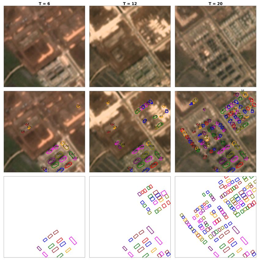
In this competition we challenged participants to identify new building construction in satellite
imagery, which could enable development policies and aid efforts by improving population esti-
mation. High-resolution population estimates help identify communities at risk for natural and
human-derived disasters. Population estimates are also essential for assessing burden on infrastruc-
ture, from roads [1] to medical facilities [2] and beyond. Organizations like the World Bank and
the World Health Organization use these estimates when evaluating infrastructure loans, grants,
and other aid programs [3]. However, population estimates are often inaccurate, out-of-date, or
non-existent in many parts of the world. In 2015, the World Bank estimated that 110 countries
globally lack effective systems for Civil Registration and Vital Statistics (CRVS), i.e. birth, death,
marriage, and divorce registration [4]. CRVS are also fundamental to assessing progress in 67 of
the 231 UN Sustainable Development Goals indicators [5]. Inaccurate population estimates can
result in poor distribution of government spending and aid distribution, overcrowded hospitals, and
inaccurate risk assessments for natural disasters [6].
    Importantly, the computer vision lessons learned from this competition could apply to other
data types. Several unusual features of satellite imagery (e.g. small object size, high object den-
sity, different color band wavelengths and counts, limited texture information, drastic changes in
shadows, and repeating patterns) are relevant to other tasks and data. For example, pathology
slide images or other microscopy data present all of the same challenges [7]. Lessons learned in
the SpaceNet Multi-Temporal Urban Development Challenge may therefore have broad-reaching
relevance to the computer vision community.

2   Novelty
To our knowledge, no past data science competition has studied deep time series of satellite imagery.
The closest comparison is the xView2 challenge [8], which examined building damage in satellite
image pairs acquired before and after natural disasters; however, this task fails to address the com-
plexities and opportunities posed by analysis of deep time series data, such as seasonal foliage and
lighting changes. Other competitions have explored time series data in the form of natural scene
video, e.g. object detection [9] and segmentation [10] tasks. There are several meaningful dissimi-
larities between these challenges and the competition described here. For example, frame-to-frame
variation is very small in video datasets (see Figure 1D). By contrast, the appearance of satellite
images can change dramatically from month to month due to differences in weather, illumination,
and seasonal effects on the ground, as shown in Figure 1C. Other time series competitions have used
non-imagery data spaced regularly over longer time intervals [11], but none focused on computer
vision tasks.
    The challenge built around the VOT dataset [12] saw impressive results for video object tracking
(e.g. [13]), yet this dataset differs greatly from satellite imagery, with high frame rates and a single
object per frame. Other datasets such as MOT17 [9] have multiple targets of interest, but still
have relatively few (< 20) objects per frame. The Stanford Drone Dataset [14] appears similar at
first glance, but has several fundamental differences that result in very different applications. That
dataset contains overhead videos taken at multiple hertz from a low elevation, and typically have
≈ 20 mobile objects (cars, people, buses, bicyclists, etc.) per frame. Because of the high frame
rate of these datasets, frame-to-frame variation is minimal (see the MOT17 example in Figure 1D).
Furthermore, objects are larger and less abundant in these datasets than buildings are in satellite
imagery. As a result, video competitions and models derived therein provide limited insight in how
to manage imagery time series with substantial image-to-image variation. Our competition and

                                                   2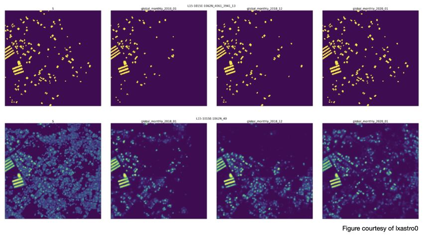
data address this gap (see Section 2 and Section 3).
    The size and density of target objects are very different in this competition than past computer
vision challenges. When comparing the size of annotated instances in the COCO dataset [15], there’s
a clear difference in object size distributions (see Figure 1A). These smaller objects intrinsically
provide less information as they comprise fewer pixels, making their identification a more difficult
task. Finally, the number of instances per image is markedly different in satellite imagery from
the average natural scene dataset (see Section 3 and Figure 1B). Other data science competitions
have explored datasets with similar object size and density, particularly in the microscopy domain
[16, 17]; however, those competitions did not address time series applications.
    Taken together, these differences (along with the use of brand-new dataset)highlight substantial
novelty for this competition.

3     Data
In this section we briefly detail the dataset used in SpaceNet 7; for a detailed description of the Multi-
temporal Urban Development (MUDS) dataset and baseline algorithm, see [18]. The SpaceNet 7
Challenge used a brand-new, open source dataset of medium-resolution (≈ 4 m) satellite imagery
collected by Planet Labs’ Dove Satellites between 2017 and 2020. The dataset is open source
this dataset under the CC-BY-4.0 ShareAlike International license. As part of AWS’s Open Data
Program1 , SpaceNet data is entirely free to download.
    The imagery comprises 24 consecutive monthly mosaic images (a mosaic is a combination of
multiple satellite images stitched together, often made to minimize cloud cover) of 101 locations over
6 continents, totaling ≈ 40, 000 km2 of satellite imagery. The dataset’s total imaged area compares
favorably to past SpaceNet challenge datasets, which covered between 120 km2 and 3, 000 km2
[19, 20, 21].
    Each image in the dataset is accompanied by two sets of manually created annotations. The
first set are GeoJSON-formatted, geo-registered building footprint polygons defining the precise
outline of each building in the image. Each building is assigned a unique identifier that persists
across the time series. The second annotations, provided in the same format, are “unusable data
masks” (UDMs) denoting areas of images obscured by clouds. Each 1024 × 1024 image has between
10 and ≈ 20, 000 building annotations, with a mean of ≈ 4, 600 (the earliest timepoints in some
geographies have very few buildings completed). This represents much higher label density than
natural scene datasets like COCO [15] (Figure 1B), or even overhead drone video datasets [22].
    The labeling process for SpaceNet 7 was an exhaustive 7-month effort that utilized both the
native Planet 4m resolution imagery, as well as higher-resolution imagery in particularly difficult
scenes. By leveraging complementary data sources, the labelers were able to create what we have
dubbed “omniscient” labels that appear to be far higher quality than what the imagery merits.
Figure 2 illustrates that in some dense scenes, label precision exceeds what the human eye could
easily distinguish in 4m resolution imagery.
    The final dataset includes ≈11M annotations, representing ∼ 500, 000 unique buildings. For the
challenge, we released 60 of the 101 AOIs (area of interest, i.e., location) for training; this portion
included both imagery and labels. Imagery (not labels) for 20 of the AOIs were released as the
“test public”. The remaining 21 AOIs were withheld as the “test private” set. Taken together, the
test set includes 4.4 million annotated buildings.
    1 https://registry.opendata.aws/spacenet/

                                                    3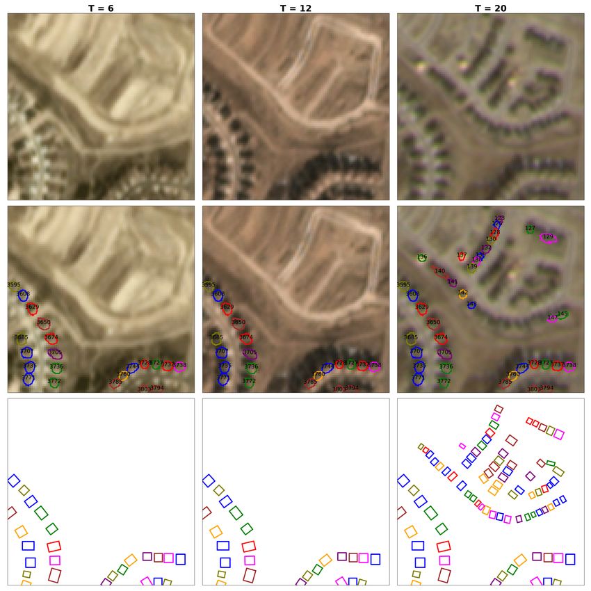
Figure 1: A comparison between our dataset and related datasets. A. Annotated objects
are very small in this dataset. Plot represents normalized histograms of object size in pixels. Blue is
our dataset, red represents all annotations in the COCO 2017 training dataset [15]. B. The density
of annotations is very high in our dataset. In each 1024 × 1024 image, our preliminary dataset
has between 10 and over 20,000 objects (mean: 4,600). By contrast, the COCO 2017 training
dataset has at most 50 objects per image. C. Three sequential time points from one geography in
our dataset, spanning 3 months of development. Compare to D., which displays three sequential
frames in the MOT17 video dataset [9].             4
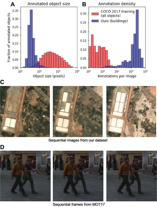
Figure 2: Zoom-in of one particularly dense SpaceNet 7 region illustrating the very high fidelity of
labels. (a) Full image. (b) Zoomed cutout. (c) Footprint polygon labels. (d) Footprints overlaid
on imagery.

4     Metric
For this competition we defined successful building footprint identifications as proposals which over-
lap ground truth (GT ) annotations with an Intersection-over-Union (IoU ) score above a threshold
of 0.25. The IoU threshold here is lower than the IoU ≥ 0.5 threshold of previous SpaceNet chal-
lenges [21, 19, 20] due to the increased difficulty of building footprint detection at reduced resolution
and very small pixel areas.
    To evaluate model performance on a time series of identifier-tagged footprints, we introduce a
new evaluation metric: the SpaceNet Change and Object Tracking (SCOT) metric. See [18] for
further details. In brief, the SCOT metric combines two terms: a tracking term and a change de-
tection term. The tracking term evaluates how often a proposal correctly tracks the same buildings
from month to month with consistent identifier numbers. In other words, it measures the model’s
ability to characterize what stays the same as time goes by. The change detection term evaluates
how often a proposal correctly picks up on the construction of new buildings. In other words, it
measures the model’s ability to characterize what changes as time goes by. The combined tracking
and change terms of SCOT therefore provide a good measure of the dynamism of each scene.

5     Challenge Structure
The competition focused on a singular task: tracking building footprints to monitor construction
and demolition in satellite imagery time series. Beyond the training data, a baseline model2 was
provided to challenge participants to demonstrate the feasibility of the challenge task. This challenge
baseline used a state-of-the-art building detection algorithm adapted from one of the prize winners
in the SpaceNet 4 Building Footprint Extraction Challenge [21]. Binary building prediction masks
are converted to instance segmentations of building footprints. Next, footprints at the same location
over the time series are be assigned the same unique identifier, see Figure 3.
    The effects and challenges associated with population estimates are myriad and very location-
dependent, and it is therefore critical to involve scientists in areas of study who rarely have access
to these data. To this end, the SpaceNet partners worked hard to lower the barrier of entry for
competing: firstly, all data for this challenge is free to download. Secondly, the SpaceNet partners
provided $25,000 in AWS compute credits to participants to enable data scientists without extensive
personal compute resources to compete. To enhance the value of these two enabling resources and
    2 https://github.com/CosmiQ/CosmiQ   SN7 Baseline

                                                        5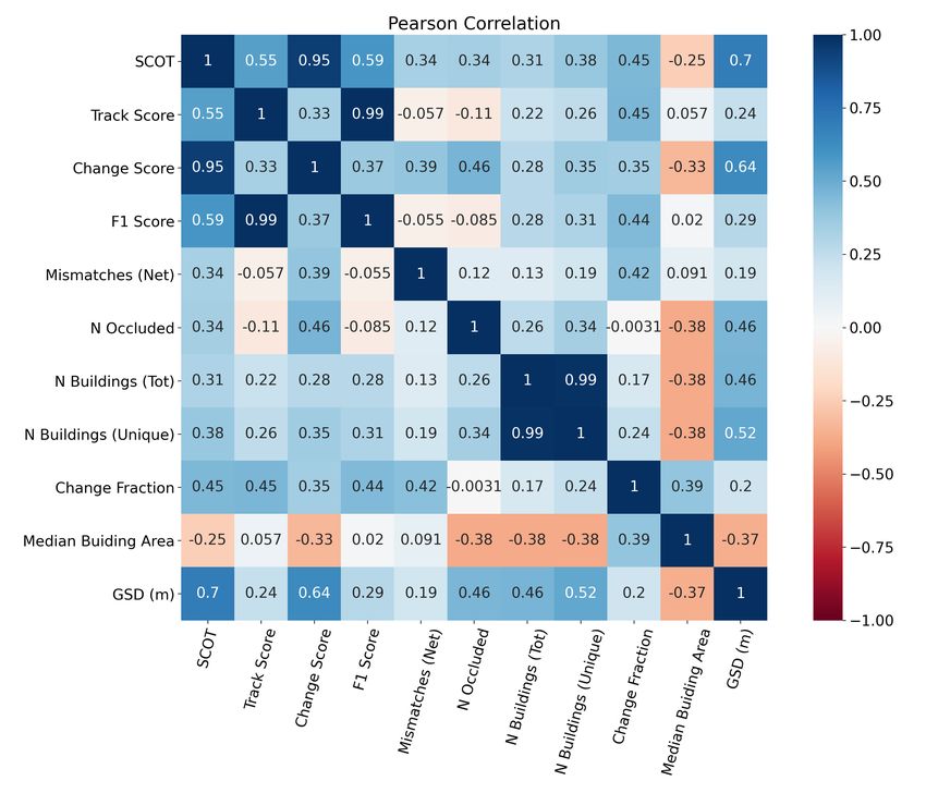
Figure 3: Baseline algorithm for building footprint extraction and identifier tracking showing evo-
lution from T = 0 (top row) to T = 5 (bottom row). Imagery (first column) feeds into the
segmentation model, yielding a building mask (second column). This mask is refined into building
footprints (third column), and unique identifiers are allocated (right column).

to further increase engagement with affected communities, we provided extensive tutorial materials
on The DownLinQ3 detailing how to download data, prepare data, run the baseline model, utilize
AWS credits, and score output predictions. We used an internationally known competition hosting
platform to ensure accessibility of the challenge worldwide (Topcoder).
    The challenge ran from September 8, 2020 - October 28, 2020. An initial leaderboard for the 311
registrants was based upon predictions submitted for the the “test public” set. The top 10 entries
on this leaderboard at challenge close were invited to submit their code in a Docker container. The
top 10 models were subsequently retrained (to ensure code was working as advertised), and then
internally tested on the “test private” set of 21 new geographies. This step of retraining the models
and testing on completely unseen data minimizes the chances of cheating, and ensures that models
are not hypertuned for the known test set. The scores on the withheld “test private” set determine
the final placings, with the winners announced on December 2, 2020. A total of $50,000 USD
was awarded to the winners (1st=$20,000 USD, 2nd=$10,000 USD, 3rd=$7,500 USD, 4th=$5,000
USD, 5th=$2,500 USD, Top Graduate=$2,500 USD, Top Undergraduate=$2,500 USD). The top-5
winning algorithms are open-sourced under a permissive license4 .

6     Overall Results
SpaceNet 7 winning submissions applied varied techniques to solving the challenge task, with the
most creativity reserved to post-processing techniques. Notably, post-processing approaches did not
simply rely upon the tried-and-true fallback of adding yet another model to an ensemble. In fact,
the winning model did not use an ensemble of neural network architectures at all, and managed an
impressive score with only a single, rapid model. Table 1 details the top-5 prize winning competitors
of the 300+ participants in SpaceNet 7.
    3 https://medium.com/the-downlinq
    4 https://github.com/SpaceNetChallenge/SpaceNet7   Multi-Temporal Solutions

                                                        6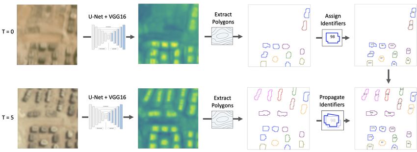
Table 1: SpaceNet 7 Results
 Competitor     Final   Total    Architectures                      #        Training   Speed
                Place   Score                                       Models   Time (H)   (km2 /min)
 lxastro0       1       41.00    1 × HRNet                          1        36         346
 cannab         2       40.63    6 × EfficienNet + UNet (siamese)   6        23         49
 selim sef      3       39.75    4 × EfficienNet + UNet             4        46         87
 motokimura     4       39.11    10 × EfficienNet-b6 + UNet         10       31         42
 MaxsimovKA     5       30.74    1 × SENet154 +UNet (siamese)       1        15         40
 baseline       N/A     17.11    1 × VGG16 + UNet                   1        10         375

Figure 4: Performance vs speed for the winning algorithms. Up and to the right is best; the1st
place algorithm is many times faster than the runner-up submissions.

    We see from Table 1 that ensembles of models are not a panacea, and in fact post-processing
techniques have a far greater impact on performance than the individual architecture chosen. The
winning algorithm is a clear leader when it comes to the combination of performance and speed, as
illustrated in Figure 4.

7    Segmentation Models
As noted above, post-processing techniques are really where the winning submissions differentiated
themselves (and will be covered in depth in Section 8), but there are a few trends in the initial deep
learning segmentation approach worth noting.

    1. Upsampling Improved Performance The moderate resolution of imagery poses a sig-
       nificant challenge when extracting small footprints, so multiple competitors upsampled the
       imagery 3 − 4× and noted improved performance.

                                                   7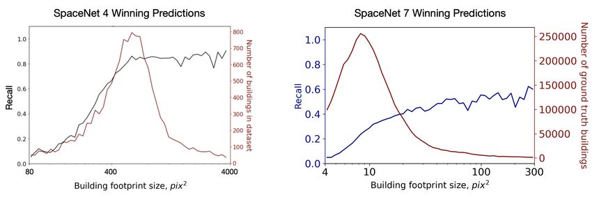
2. 3-channel Training Mask The small pixel sizes of many buildings results in very dense
       clustering in some locations, complicating the process of footprint extraction. Accordingly,
       multiple competitors found utility in 3-channel “footprint, boundary, contact” (fbc5 ) segmen-
       tation masks for training their deep learning models.
    3. Ensembles Remain the Norm While the winning algorithm eschewed multi-model ensem-
       bles (to great speed benefits), the remainder of the top-4 competitors used an ensemble of
       segmentation models which were then averaged to form a final mask.

8     Winning Approach
While there were interesting techniques adopted by all the winning algorithms, the vastly superior
speed of the winning algorithm compared to the runners-up merits a closer look. The winning team
of lxastro0 (consisting of four Baidu engineers) improved upon the baseline approach in three key
ways.
    1. They swapped out the VGG16 [23] + U-Net [24] architecture of the baseline with the more
       advanced HRNet [25], which maintains high-resolution representations through the whole
       network. Given the small size of the SpaceNet 7 buildings, mitigating the downsampling
       present in most architectures is highly desirable.
    2. The small size of objects of interest is further mitigated by upsampling the imagery 3× prior
       to ingestion into HRNet. The team experimented with both 2× and 3× upsampling, and
       found that 3× upsampling proved superior.
    3. Finally, and most crucially, the team adopted an elaborate post-processing scheme they term
       ”temporal collapse” which we detail in Section 8.1.

8.1      Temporal Collapse
In order to improve post-processing for SpaceNet 7, the winning team assumed:
    1. Buildings will not change after the first observation.
    2. In the 3× scale, there is at least a one-pixel gap between buildings.

    3. There are three scenarios for all building candidates:
        (a) Always exists in all frames
        (b) Never exists in any frame
         (c) Appears at some frame k and persists thereafter

   The data cube for each AOI can be treated as a video with a small (∼ 24) number of frames.
Since assumption (1) states that building boundaries are static over time, lxastro0 compresses the
temporal dimension and predicts the spatial location of each building only once, as illustrated in
Figure 5a.
    5 https://solaris.readthedocs.io/en/latest/tutorials/notebooks/api   masks tutorial.html

                                                          8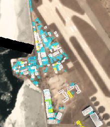
(a)                                                 (b)

Figure 5: (a) Visualization of temporal collapse for ground truth (top row) and predictions (bottom
row). The left frame is the compressed probability map. (b) Method for determining the temporal
origin of an individual building. Top row: The three possible scenarios of assumption (c). Bottom
row: The aggregated predicted probability for the building footprint at each time step (blue) is
used to map to the final estimated origin (red).

                                   Table 2: baseline model vs lxastro0
                                Metric          baseline      lxastro0
                                F1              0.46 ± 0.13   0.61 ± 0.09
                                Track Score     0.41 ± 0.11   0.61 ± 0.09
                                Change Score    0.06 ± 0.06   0.20 ± 0.09
                                SCOT            0.17 ± 0.11   0.41 ± 0.11

    Building footprint boundaries are extracted from the collapsed mask using the watershed algo-
rithm and an adaptive threshold, and taking into account assumption (2). This spatial collapse
ensures that predicted building footprint boundaries remain the same throughout the time series.
With the spatial location of each building now determined, the temporal origin must be computed.
At each frame, and for each building, the winning team averaged the predicted probability values
at each pixel inside the pre-determined building boundary. This mapping is then used to determine
at which frame the building originated, as illustrated in Figure 5b.
    The techniques adopted by lxastro0 yield marked improvements over the baseline model in all
metrics, but most importantly in the change detection term of the SpaceNet Change and Object
Tracking (SCOT) metric. See Table 2 for quantitative improvements. Figure 6a illustrates predic-
tions in a difficult region, demonstrating that while the model is imperfect, it does do a respectable
job given the density of buildings and moderate resolution. We discuss Figure 6b in Section 8.2.

8.2    Feature Correlations
There are a number of features of the dataset and winning prediction that are worth exploring.
Figure 7a displays the correlation between various variables across the AOIs for the winning submis-
sion. Most variables are positively correlated with the total SCOT score. Note the high correlation
between SCOT and the change score; since change detection is much more difficult this term ends
up dominating.

                                                   9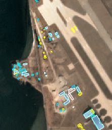
(a) (b)
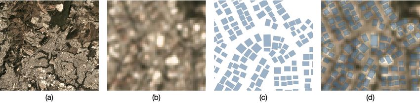
Figure 6: Imagery, predictions and ground truth. Input imagery (top row), predictions
(middle row), and ground truth (bottom row) of the winning model for sample test regions. The
left column denotes month 6 (October 2018), with the middle column 6 months later and the right
column another 8 months later. (a) AOI 1, latitude = 20◦ , change score = 0.30. (b) AOI 2, latitude
= 40◦ , change score = 0.09.
There are a number of intriguing correlations in Figure 7a, but one unexpected finding was the
high (+0.7) correlation between ground sample distance (GSD), and SCOT. This correlation is even
stronger than the correlation between SCOT and F1 or SCOT and track score. GSD is the pixel
size of the imagery, so a higher GSD corresponds to larger pixels and lower resolution. Furthermore,
since all images are the same size in pixels (1024 × 1024), a larger GSD will cover more physical
area, thereby increasing the density of buildings. Therefore, one would naively expect an inverse
correlation between GSD and SCOT where increasing GSD leads to decreased SCOT, instead of
the positive correlation of Figure 7a.
As it turns out, the processing of the SpaceNet 7 Planet imagery results in GSD ≈ 4.8m ×
Cos(Latitude). Therefore latitude (or more precisely, the absolute value of latitude) is negatively
correlated with tracking (-0.39), change (-0.65) and SCOT (-0.70) score. Building footprint tracking
is apparently more difficult at higher latitudes, see Figure 7b.
The high negative correlation (-0.65) between the change detection term (change score) and
latitude is noteworthy. Evidently, identifying building change is significantly harder at higher
latitudes. We leave conclusive proof of the reason for this phenomenon to further studies, but
hypothesize that the reason is due to the greater seasonality and more shadows/worse illumination
(due to more oblique sun angles) at higher latitudes. Figure 6b illustrates some of these effects.
Note the greater shadows and seasonal change than in Figure 6a. For reference, the change score
for Figure 6a (latitude of 20 degrees) is 0.30, whereas the change score for Figure 6b (latitude of 40
degrees) is 0.09.
10(a) Pearson Correlations (b) SCOT vs latitude
Figure 7: Correlations (a) and scatter plot (b) for the winning submission.
8.3 Performance Curves
Object size is an important predictor of detection performance, as noted in a number of previous
investigations (e.g. [26]). We follow the lead of analyses first performed in SpaceNet 4 [27] (and
later SpaceNet 6 [28]) in exploring object detection performance as function of building area. Figure
8 shows performance for all 4.4 million building footprints in the SpaceNet 7 public and private
test sets for the winning submission of team lxastro0.
The pixel size of objects is also of interest, particularly in comparison to previous SpaceNet
challenges. The SpaceNet 4 Challenge used 0.5m imagery, so individual pixels are 1/64 the area of
our 4m resolution SpaceNet 7 data, yet for SpaceNets 4 and 7 the physical building sizes are similar
[29]. Figure 9 plots pixel sizes directly (for this figure we adopt IoU ≥ 0.5 for direction comparisons),
demonstrating the far superior pixel-wise performance of SpaceNet 7 predictions in the small-area
regime (∼ 5× greater for 100 pix2 objects), though SpaceNet 4 predictions have a far higher score
ceiling. The high SpaceNet 7 label fidelity (see Figure 2) may help explain the over-achievement of
the winning model prediction on small buildings. SpaceNet 7 labels encode extra information not
Figure 8: Building recall as a function of area for the winning submission (IoU ≥ 0.25).
11Figure 9: Prediction performance as a function of building pixel area (IoU ≥ 0.5).
1.0 0.5
1 - lxastro0
2 - cannab 0.4 0.5 0.6 21 0.7
3 - selim_sef 0.9
0.8 4 - motokimura 0.4 7
5 - MaksimovKA 0.8 20
21
baseline 0.7 21 21
Change Detection Score
0.6 Change Detection Score 1 7
0.6 0.3 1 7
3
0.5 20 20
5 321 8 77
4 14
0.4 20
4 14
3 1714
3 17
10
0.4 0.3 0.2 20 16 4
14 1410 10
8
8
3 17 8 2
1 10 2
18 159 9 92
5
1 16
0.2 5 19 18 18
4 1717 9 13
13 13
12 12
16 4 16 18 8 12 15
10 12
13
15
0.2 0.1 0.1 1 16 11 5 15
19 2 12
5 13
11 11 19
19 9
1815 2 19 66
11 11 6
6 6
0.0 0.0
0.0 0.2 0.4 0.6 0.8 1.0 0.4 0.5 0.6 0.7 0.8
Tracking Score Tracking Score
(a) By model (b) By AOI
Figure 10: Change score vs. tracking score for each combination of model and AOI, color-coded
(a) by model and (b) by AOI. Contour lines indicate SCOT score.
obvious to humans in the imagery, which models are apparently able to leverage. Of course there is
a limit (hence the score ceiling of SpaceNet 7 predictions), but this extra information does appear
to help models achieve surprisingly good performance on difficult, crowded scenes.
8.4 SCOT Analysis
Comparing the performance of the various models can give insight into the role played by the two
terms that make up the SCOT metric. Figure 10a plots change detection score against tracking
score for each model in Table 1, showing a weak correlation. Breaking down those points by
AOI in Figure 10b shows that deviations from linearity are largely model-independent, instead
relating to differences among AOIs. The AOIs labeled “20” and “12” show extreme cases of this
variation (Figure 11). AOI 20 achieves a high change detection score despite a low tracking score
because many buildings are detected either from first construction or not at all. AOI 12, on the
12(a) AOI 20 before (b) AOI 20 after (c) AOI 12 before (d) AOI 12 after
Figure 11: Detail of AOI 20 (a) before and (b) after the completion of new construction, and
similarly for AOI 12 (c) before and (d) after. Matched footprints are in white, false positives in
yellow, and false negatives in blue.
other hand, achieves a high tracking score despite a low change detection score because predicted
building footprints often appear earlier than ground truth, potentially an effect of construction
activity. Such cases show the value in using both terms to make SCOT a holistic measure of model
performance.
9 Conclusions
The winners of The SpaceNet 7 Multi-Temporal Urban Development Challenge all managed im-
pressive performance given the difficulties of tracking small buildings in medium resolution imagery.
The winning team submitted by far the most and rapid (and therefore the most useful) proposal. By
executing a “temporal collapse” and identifying temporal step functions in footprint probability, the
winning team was able to vastly improve both object tracking and change detection performance.
Inspection of correlations between variables unearthed an unexpected decrease in performance with
increasing resolution. Digging into this observation unearthed that the latent variable appears to
be latitude, such that SCOT performance degrades at higher latitudes. We hypothesize that the
the greater lighting differences and seasonal foliage change of higher latitudes complicates change
detection. Predictions for the SpaceNet 7 4m resolution dataset perform surprisingly well for very
small buildings. In fact, Figure 9 showed that prediction performance for 100 pix2 objects is ∼ 5×
for SpaceNet 7 than for SpaceNet 4. The high fidelity “omniscient” labels of SpaceNet 7 seem
to aid models for very small objects, though the lower resolution of SpaceNet 7 results in a lower
performance ceiling for larger objects. Insights such as these have the potential to help optimize
collection and labeling strategies for various tasks and performance requirements.
Ultimately, the open source and permissively licensed data and models stemming from SpaceNet
7 have the potential to aid efforts to improve mapping and aid tasks such as emergency preparedness
assessment, disaster impact prediction, disaster response, high-resolution population estimation,
and myriad other urbanization-related applications.
13References
[1] Chen, S., Kuhn, M., Prettner, K., Bloom, D.E.: The global macroeconomic burden of road
injuries: estimates and projections for 166 countries. (2019)
[2] Schuurman, N., Fiedler, R.S., Grzybowski, S.C., Grund, D.: Defining rational hospital catch-
ments for non-urban areas based on travel time. 5 (2006)
[3] World Bank Group, T.: World Bank Annual Report 2019. The World Bank (2019)
[4] Mills, S.: Civil registration and vital statistics: key to better data on maternal mortality (Nov
2015)
[5] Mills, S., Abouzahr, C., Kim, J., Rassekh, B.M., Sarpong, D.: Civil registration and vital
statistics (crvs) for monitoring the sustainable development goals (sdgs). (2017)
[6] Guha-Sapir, D., Hoyois, P. In: Estimating populations affected by disasters: A review of
methodological issues and research gaps. United Nations Sustainable Development Group
(March 2015)
[7] Weir, N., Ben-Joseph, J., George, D.: Viewing the world through a straw: How lessons from
computer vision applications in geo will impact bio image analysis (Jan 2020)
[8] Gupta, R., Hosfelt, R., Sajeev, S., Patel, N., Goodman, B., Doshi, J., Heim, E., Choset, H.,
Gaston, M.: Creating xbd: A dataset for assessing building damage from satellite imagery.
In: Proceedings of the 2019 CVF Conference on Computer Vision and Pattern Recognition
Workshops. (2019)
[9] Leal-Taixé, L., Milan, A., Schindler, K., Cremers, D., Reid, I.D., Roth, S.: Tracking the
trackers: An analysis of the state of the art in multiple object tracking. CoRR abs/1704.02781
(2017)
[10] Caelles, S., Pont-Tuset, J., Perazzi, F., Montes, A., Maninis, K.K., Van Gool, L.: The 2019
davis challenge on vos: Unsupervised multi-object segmentation. arXiv:1905.00737 (2019)
[11] Google: Web traffic time series forecasting: Forecast future traffic to wikipedia pages
[12] Kristan, M., Matas, J., Leonardis, A., Vojir, T., Pflugfelder, R., Fernandez, G., Nebehay,
G., Porikli, F., Čehovin, L.: A novel performance evaluation methodology for single-target
trackers. IEEE Transactions on Pattern Analysis and Machine Intelligence 38(11) (Nov 2016)
2137–2155
[13] Wang, Q., Zhang, L., Bertinetto, L., Hu, W., Torr, P.H.: Fast online object tracking and
segmentation: A unifying approach. In: The IEEE Conference on Computer Vision and
Pattern Recognition (CVPR). (June 2019)
[14] Robicquet, A., Sadeghian, A., Alahi, A., Savarese, S.: Learning social etiquette: Human
trajectory understanding in crowded scenes. In: ECCV. (2016)
[15] Lin, T., Maire, M., Belongie, S.J., Bourdev, L.D., Girshick, R.B., Hays, J., Perona, P., Ra-
manan, D., Dollár, P., Zitnick, C.L.: Microsoft COCO: common objects in context. CoRR
abs/1405.0312 (2014)
14[16] Recursion Pharmaceuticals: Cellsignal: Disentangling biological signal from experimental noise
in cellular images
[17] Hamilton, B.A., Kaggle: Data science bowl 2018: Spot nuclei. speed cures.
[18] Van Etten, A., Hogan, D., Martinez-Manso, J., Shermeyer, J., Weir, N., Lewis, R.: The
multi-temporal urban development spacenet dataset (2021)
[19] Van Etten, A., Lindenbaum, D., Bacastow, T.M.: Spacenet: A remote sensing dataset and
challenge series. CoRR abs/1807.01232 (2018)
[20] Van Etten, A., Shermeyer, J., Hogan, D., Weir, N., Lewis, R.: Road network and travel time
extraction from multiple look angles with spacenet data (2020)
[21] Weir, N., Lindenbaum, D., Bastidas, A., Van Etten, A., McPherson, S., Shermeyer, J., Vijay,
V.K., Tang, H.: Spacenet MVOI: a multi-view overhead imagery dataset. In: Proceedings of
the 2019 International Conference on Computer Vision. Volume abs/1903.12239. (2019)
[22] Stanford Computational Vision and Geometry Lab: Stanford drone dataset
[23] Simonyan, K., Zisserman, A.: Very deep convolutional networks for large-scale image recogni-
tion. In: Proceeings of the 2015 International Conference on Learning Representations. (2015)
[24] Ronneberger, O., Fischer, P., Brox, T.: U-net: Convolutional networks for biomedical im-
age segmentation. In: Proceedings of the 2015 International Conference on Medical Image
Computing and Computer-Assisted Intervention. (2015)
[25] Wang, J., Sun, K., Cheng, T., Jiang, B., Deng, C., Zhao, Y., Liu, D., Mu, Y., Tan, M., Wang,
X., Liu, W., Xiao, B.: Deep high-resolution representation learning for visual recognition
(2020)
[26] Van Etten, A.: You only look twice: Rapid multi-scale object detection in satellite imagery
(2018)
[27] Weir, N.: The good and the bad in the spacenet off-nadir building footprint extraction challenge
(Feb 2019)
[28] Shermeyer, J.: Spacenet 6: A first look at model performance (Jun 2020)
[29] Van Etten, A.: Spacenet 7 results: Overachieving pixels (Jan 2021)
15You can also read