Phaseless Radar Coincidence Imaging with a MIMO SAR Platform - MDPI
←
→
Page content transcription
If your browser does not render page correctly, please read the page content below
remote sensing
Article
Phaseless Radar Coincidence Imaging with a MIMO
SAR Platform
Aaron V. Diebold * , Mohammadreza F. Imani            and David R. Smith
 Department of Electrical and Computer Engineering, Duke University, Durham, NC 27708, USA;
 mohamad.imani@gmail.com (M.F.I.); drsmith@ee.duke.edu (D.R.S.)
 * Correspondence: aaron.diebold@duke.edu

 Received: 8 January 2019; Accepted: 27 February 2019; Published: 5 March 2019

 Abstract: The correlation-based synthetic aperture radar imaging technique, termed radar coincidence
 imaging, is extended to a fully multistatic multiple-input multiple-output (MIMO) synthetic aperture
 radar (SAR) configuration. Within this framework, we explore two distinct processing schemes:
 incoherent processing of intensity data, obtained using asynchronous receivers and inspired by optical
 ghost imaging works, and coherent processing with synchronized array elements. Improvement in
 resolution and image quality is demonstrated in both cases using numerical simulations that model
 an airborne MIMO SAR system at microwave frequencies. Finally, we explore methods for reducing
 measurement times and computational loads through compressive and gradient image reconstruction
 using phaseless data.

 Keywords: ghost; RCI; correlation; radar; coincidence; imaging; MIMO; SAR

1. Introduction
     Radar coincidence imaging (RCI) is a recently proposed microwave imaging approach that
applies principles of ghost imaging in a radar array or synthetic aperture radar (SAR) framework [1].
Whereas conventional SAR systems employ a single transceiver to interrogate a target as the radar
platform moves along a synthetic aperture path (monostatic acquisition), a hallmark of RCI is the
simultaneous use of a collection of transmitters and/or receivers for rapid multistatic signal acquisition.
To date, multiple-input single-output (MISO) [1–4] or single-input multiple-output (SIMO) [5] RCI
systems have been put forth as candidates for achieving incoherent measurement patterns required
in a ghost imaging scheme through a superposition of approximately time- and space-independent
waveforms. In these cases, approximately uncorrelated measurement patterns can be guaranteed
through stochastic modulation of the transmitted signals. This offers the added benefit of introducing
natural anti-jamming qualities to the radar system [6].
     The ability to implement RCI in MISO or SIMO configurations indicates that it can be handled
more generally under a fully multiple-input multiple-output (MIMO) formulation. MIMO radar
involves leveraging the large number of degrees of freedom offered by transmitting and receiving
arrays for improved system performance in terms of resolution or detection capabilities [7,8].
Instead of sequentially switching through each channel in the MIMO system, significant effort has
gone into investigating orthogonal coding schemes in order to access these additional degrees of
freedom for post processing [8–13]. This enables rapid signal acquisition through simultaneous
illumination and reception among all of the array elements, with the potential for high-speed
and high-resolution, wide-swath radar. In proposed systems, exploiting the additional degrees of
freedom for improved image resolution requires coherent processing [8], which demands sophisticated
synchronization capabilities between the transmitting and receiving array elements [14–17]. In answer
to the above requirements, RCI can handle the signal extraction problem naturally through a

Remote Sens. 2019, 11, 533; doi:10.3390/rs11050533                      www.mdpi.com/journal/remotesensing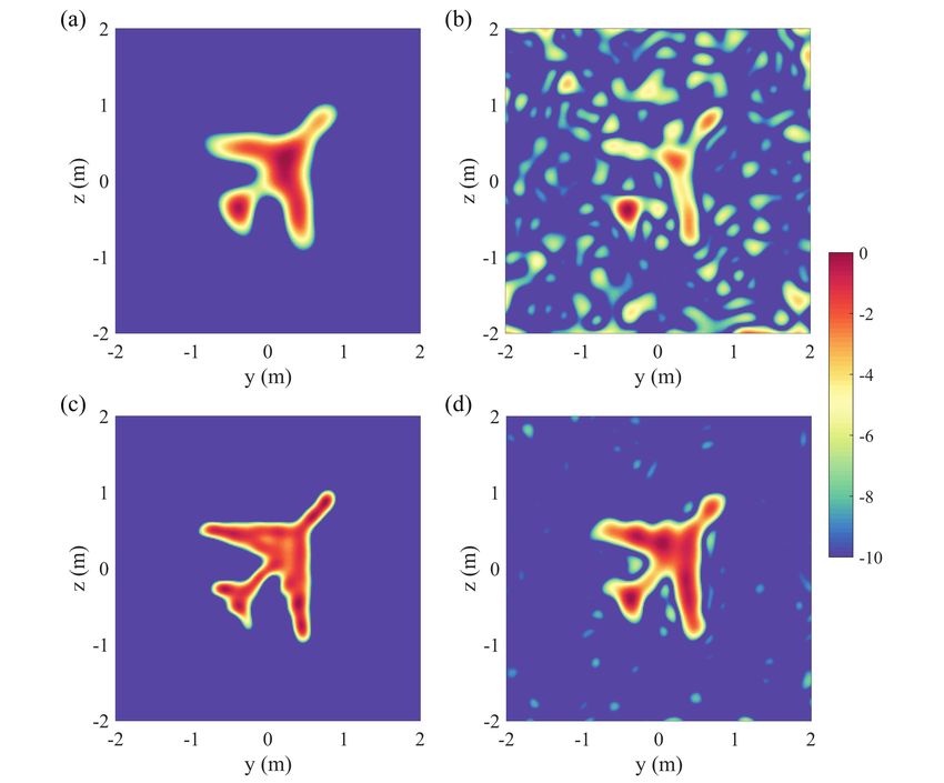
Remote Sens. 2019, 11, 533                                                                              2 of 15

correlation-based image reconstruction method that is well-established in multiplexing computational
imaging systems [18]. The further degrees of freedom of the MIMO system in this case enter into the
problem implicitly through the spatial incoherence of the combined illuminating fields, which become
approximately orthogonal in the limit of a dense transmitting array. In addition, by noting the
relationship of RCI to the optical ghost imaging method, we will see that incoherent processing of RCI
data can significantly alleviate synchronization requirements for high-resolution MIMO imaging.
      In optical ghost imaging experiments, an image is recovered through a correlation between
the spatially varying transmitted intensity patterns and a set of backscatter intensity measurements
collected by a single detector [19]. Computational ghost imaging [20,21] employs known, computable
patterns, and the correlation is performed with respect to a set of distinct patterns. Such an architecture
achieves lenseless, single-pixel imaging directly from intensity measurements, which can be highly
advantageous given the restrictions of optical detection hardware. Nevertheless, the relative ease
of measuring phase at microwave frequencies has encouraged reconstruction through full-field
(phase and amplitude) correlations, or other inversion techniques, in most RCI demonstrations. In this
context, RCI can be viewed as a multistatic implementation of time-domain correlation with pulse
diversity [6]. While it is true that full-field correlations can achieve improved image convergence
rates over their phaseless counterparts [22], several unique advantages have been documented for
the phaseless optical ghost imaging approach [23–25] that have not been adequately explored in
the microwave radar setting. These include a robustness to turbulence on the receive arm and the
removal of synchronization requirements between source and receiver. In addition, RCI proposals
have primarily utilized ground-based radar configurations. With the advent of metasurface antennas,
many of the daunting hardware bottlenecks facing both ground-based and airborne MIMO SAR
systems can be circumvented [26,27]. Dynamic metasurface apertures [28–32] in particular stand
as a versatile, low-cost and lightweight technology that can facilitate the necessarily large-scale
framework supporting MIMO SAR techniques. We thus propose RCI on a MIMO SAR platform,
investigate the differences between full-field and phaseless modalities, and identify advantages
of each scheme. In particular, we show that full-field reconstruction achieves superior imaging
performance, while phaseless reconstruction can alleviate hardware synchronization requirements
as well as computational demands and phase error artifacts in reconstructions. Motivated by the
advantages offered by phaseless imaging, we also investigate compressive techniques. Furthermore,
considering the inherent motion of an airborne SAR system, we propose an approach which leverages
array motion to directly achieve edge detection of targets. Its advantages are examined in the context
of phaseless and compressive reconstruction. While the economic advantages of the aforementioned
technologies help motivate this analysis, we remain agnostic to the particular hardware approach and
focus on new acquisition and processing possibilities enabled by MIMO SAR.
      In what follows, we detail the MIMO SAR imaging configuration as well as the RCI reconstruction
formulation. We investigate the effects of array geometry on the imaging point spread function and
the resulting imaging performance. Phaseless and full-field correlation reconstructions are compared,
as well as results of applying more advanced reconstruction techniques. Finally, we outline various
system differences between the two cases, such as synchronization requirements and effects of
phase error.

2. Results

2.1. Imaging Configuration
     The imaging geometry employed in this work is shown in Figure 1. For the sake of presentation,
we consider in this paper an airborne MIMO SAR scenario in which a collection of N = 40 airborne
transmitters (investigated in Section 2.2.1), e.g., a constellation of transmitting UAVs, fly at an altitude of
x = 2 km in the yz plane, parallel to the two-dimensional region of interest. We assume all transmitters
at a given time are constrained within a 200 by 200 m2 area with positions given by ~r Tn (t) with
Remote Sens. 2019, 11, 533                                                                               3 of 15

n = 1, ..., N, where we allow the transmitter positions to vary with time to reflect the fact that different
pulses may originate from different positions along the constellation trajectory. Each transmitter
traverses a total distance of 40 m. We make a stop-and-shoot approximation throughout this work,
neglecting effects of motion during a pulse and assuming stationary transmitters/receivers during a
pulse. The number of receivers K within the constellation will vary depending on the implementation,
and their positions will similarly be allowed to vary in time.

      Figure 1. (a) Side view of layout for airborne radar coincidence imaging (RCI). (b) Diagonal view of
      layout for airborne RCI, including example intensity patterns at different times within a pulse.

     Each transmitting source emits an amplitude-, phase- and frequency-modulated pulsed signal
with a frequency range of 9.5–9.8 GHz sampled at 15 MHz. The pulse waveform emitted from the nth
transmitter, sn (t), is modeled as [1]

                                         Q
                                                            t − qτp
                             sn (t) =   ∑ A(t)rect(            T
                                                                    )exp[ j(2π f (t)t + φ(t))]               (1)
                                        q =1

where the amplitude A(t), frequency f (t) and phase φ(t) are stochastically-varying with uniform
distributions on the intervals [0, 1], [9.5 GHz, 9.8 GHz] and [−π, π ], respectively. These parameters
fluctuate within a single pulse, as well as over the entire waveform/acquisition time (i.e., across all
constellation positions). T indicates the pulse duration, which is taken to be 1 µs, and τp is the
pulse repetition interval. q = 1, ..., Q indexes a single pulse within the waveform, so that Qτp is
the total acquisition time. Unless otherwise stated, we model the acquisition process with a single
transmitted pulse per each equispaced constellation position, for a total of Q = 50 pulses/positions.
The transmitters are assumed to be phase-synchronized, and illuminate the scene simultaneously.
Under this condition, the superposition of their pulses, s(~r, t), at each position ~r of the imaging domain
can be computed for every instance of time t:

                                                        N
                                                                     |~r −~r Tn (t)|
                                          s(~r, t) =   ∑ sn (t −            c
                                                                                     )                       (2)
                                                       n =1

where c is the speed of light.
     The scene to be reconstructed is represented by a spatially-varying scattering density σ (~r )
that occupies a 4 m by 4 m area. While such a constrained region of interest is not practically
achievable, the results obtained for this scenario can be generalized through proper scaling and
sampling. We restrict ourselves to such a limited area in this work due to computational limitations.
Remote Sens. 2019, 11, 533                                                                                    4 of 15

We assume a non-fluctuating target model, so that σ (~r ) is a deterministic, unknown quantity [33].
The scattered signal, under the first Born approximation, is s(~r, t)σ (~r ). The signal s Rk (t) measured by
receiver k, k = 1, ..., K, located at position ~r Rk (t), is given by a sum over this scattered signal modified
by the appropriate propagation delay:

                                                      |~r Rk (t) −~r |
                                          Z
                             s Rk (t) =       σ (~r )s(~r, t −         )dV
                                                               c
                                                N
                                                            |~r −~r Tn (t)| |~r Rk (t) −~r |
                                       Z
                                      = σ(~r ) ∑ sn (t −                   −                 )dV                 (3)
                                               n =1
                                                                   c                c
                                          Z
                                      =       σ (~r )sre f ,k (~r, t)dV

where V indicates the region of interest to be imaged, and the reference signal for receiver k, sre f ,k , is
defined as
                                             N
                                                      |~r −~r Tn (t)| |~r Rk (t) −~r |
                         sre f ,k (~r, t) = ∑ sn (t −                −                 ).                (4)
                                            n =1
                                                             c                c

     When N is sufficiently large, these reference fields are expected to be spatially incoherent [1] and
to approximately obey speckle statistics [34], while temporal incoherence is guaranteed through the
stochastic fluctuations of each transmitted signal. Spatial and temporal incoherence are characterized
by the condition              Z
                                         ∗                            0                         0
                                  κ     sre f ,k (~r, t ) sre f ,k (~r , t + τ ) dt ≈ Nδ (~r −~r ) δ ( τ ).      (5)

where we are considering our reference fields to be stationary in time. κ = ( t dt)−1 is a normalization
                                                                             R

factor characterizing the length of the acquisition interval. In the remainder of this work, we will
generally ignore constant normalization terms unless required for clarity. The magnitudes of two
example reference patterns are depicted in Figure 2a,b, illustrating the speckle nature of the fields for
large N.

      Figure 2. (a) Example reference pattern for N = 10 transmitters. (b) Example reference pattern for
      N = 40 transmitters. (c) singular value decomposition (SVD) of complex reference fields as N is varied.
      (d) y-slice of center-position spatial autocorrelation as N is varied.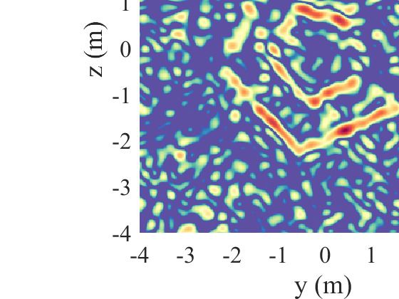
Remote Sens. 2019, 11, 533                                                                                                                                                          5 of 15

   For computational purposes, we can equivalently define these reference fields in the frequency
domain as                                                j2π f
                                      N

                                                     exp − c |~r −~r Tn (ts )| + |~r Rk (ts ) −~r |
            Sre f ,k (~r, f , ts ) = ∑ Sn ( f , ts )                                                  (6)
                                     n =1
                                                            |~r −~r Tn (ts )||~r Rk (ts ) −~r |
where Sn ( f , ts ) is the temporal Fourier transform of sn (t) with respect to the fast time (i.e., the signal
temporal variation), and ts denotes the slow time that characterizes the constellation motion.

2.2. Reconstruction

2.2.1. Single Receiver
     Several works to date have demonstrated RCI using a single-receiver (K = 1) configuration [1–4].
We similarly choose this case as our starting point, since many characteristics of the RCI approach
can be intuitively understood and adequately described under such a configuration. We denote the
single receiver position ~r R (t), its measured signal s R (t) and its reference signal sre f (~r, t). In RCI using
complex measurements, an image Gc (~r ) is obtained through a complex cross-correlation between the
measured signal and the reference signals. In the time domain, this correlation is
                                                                              Z
                                                                                       ∗
                                                                 Gc (~r ) =           sre f (~r, t ) s R ( t ) dt.                                                                     (7)
                                                                                  t

     In Equation (7), the correlation is performed over the total acquisition time Qτp , which includes
all positions traversed by the array. Under the large N assumption, sre f (~r, t) is spatially incoherent [1].
For stochastic signals, the large N assumption further guarantees circular complex Gaussian statistics,
which ensures the spatial incoherence of the reference field intensities through the complex Gaussian
moment theorem [22] paired with Equation (5):
    Z                                                       Z                                                   Z                              Z
            |sre f (~r, t)|2 |sre f (~r 0 , t)|2 dt = κ |         ∗
                                                                 sre                     0          2
                                                                     f (~r, t ) sre f (~r , t ) dt | + κ                |sre f (~r, t)|2 dt             |sre f (~r 0 , t0 )|2 dt0
        t                                                    t                                                      t                              t0                                  (8)
                                                     ≈ κN δ(~r −~r 0 ) + const.
                                                             2

where the field intensities for scalar, complex signals f (~r, t) are defined as | f (~r, t)|2 = f (~r, t)∗ f (~r, t).
In optical ghost imaging implementations, this condition motivates image formation with an
approximately equivalent phaseless correlation of intensity fluctuations G pl (~r ) [19]:
                                             Z                                                  Z                             Z
                              G pl (~r ) =                         2           2
                                                     |sre f (~r, t)| |s R (t)| dt − κ                                    2
                                                                                                        |sre f (~r, t)| dt             |s R (t0 )|2 dt0 .                              (9)
                                                 t                                                  t                             t0

       In the following, we will examine various requirements on phaseless imaging in an RCI setting.
       As in [1], we may discretize our reference and received waveforms into M discrete increments
ti , i = 1, ..., M of length 1/BW, where BW is the frequency bandwidth. For Q = 50 pulses/positions,
this results in M = 15, 000 total scattered field samples. Our region of interest can be discretized into P
pixels at positions ~r j , j = 1, ..., P. Then we can write the forward model describing our measurements
in Equation (3) as
                                                      s = Hσ                                           (10)

where s is the M × 1 vector of measurements, si = s R (ti ), σ is the P × 1 vector describing the
discretized scattering density, σj = σ (~r j ), and the M × P matrix H is the matrix of reference fields with
Hij = sre f (~r j , ti ). Then the time-domain correlation of Equation (7) can be written as

                                                                            σ est = H† s.                                                                                            (11)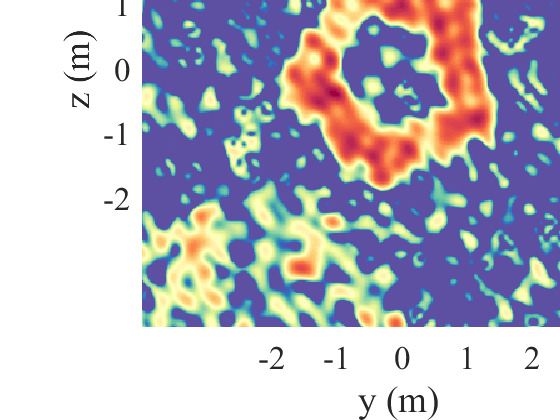
Remote Sens. 2019, 11, 533 6 of 15
where † denotes the conjugate transpose. Similarly, due to the equivalent expression of the covariance
calculation in Equation (9) as
Z Z Z
2 0 2 0 2 00 2 00
G pl (~r ) = (|sre f (~r, t)| − κ |sre f (~r, t )| dt )(|s R (t)| − κ |s R (t )| dt ) dt, (12)
t t0 t00
we can write the phaseless correlation of Equation (9) as
T
σ̂ est = Ĥ ŝ (13)
where σ̂ est is the estimated intensity scattering response, and Ĥ and ŝ consist of the reference and
measured intensities, respectively:
M
1
Ĥij = | Hij |2 −
M ∑0 | Hi0 j |2
i
(14)
M
1
ŝi = |si |2 −
M ∑0 |si0 |2
i
Substitution of Equation (3) into Equation (7) reveals that the spatially-varying point spread
function for the complex RCI system is given by the complex spatial autocorrelation of the reference
fields, H† H. In a phaseless RCI system, the point spread function is given approximately (exactly,
T
in the limit of an incoherent system [35,36]) by the intensity autocorrelation Ĥ Ĥ. A significant
result of this distinction is the loss of the ability to perform aperture synthesis through constellation
motion in phaseless RCI. That is, phase contributions only occur in the phaseless system during the
computation of the reference intensity pattern |sre f (~r, t)|2 for each position. Since data from distinct
trajectory positions is not coherently processed, the phaseless system point spread function is not
sensitive to phase differences between the reference patterns corresponding to different positions in
the trajectory. Instead, different trajectory positions contribute only by means of a much more slowly
varying amplitude decay. This means that the resolving capabilities of the phaseless RCI system largely
depend on the instantaneous array geometry, in contrast to the resolution in complex RCI which is
determined by the total range of sampled positions achieved within the coherent integration time.
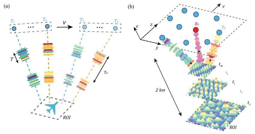
This fact is illustrated in Figure 3.
Figure 3a illustrates a linear array oriented along the y axis and moving along the z direction.
At each position along the constellation trajectory, all transmitting elements simultaneously emit a
pulse, and the collective backscattered signal is measured by a single receiver. Figure 3b shows the
complex point spread function evaluated at the center of the region of interest, i.e., the image of a
point reconstructed through Equation (7). The point is well-resolved in both directions due to the fact
that the linear array combined with constellation motion has synthesized a two-dimensional array.
In contrast, the result of phaseless reconstruction through Equation (9) is depicted in Figure 3c. Here,
the point is resolved well along the direction of the linear array orientation, but is unresolved along the
direction of array motion. These results correspond to the fact that while the phase diversity attained
by the array along the y direction yields significant interferometric variation in the intensities along
that direction for a given constellation position, insufficient instantaneous phase variation is achieved
in the reference signals along the z direction, so that the phaseless system resolution in the z direction
is defined only by the amplitude decay induced by array motion.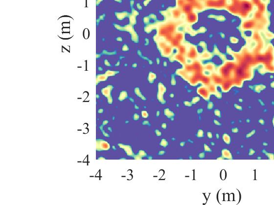
Remote Sens. 2019, 11, 533                                                                                    7 of 15

      Figure 3. (a) Linear multiple-input single-output (MISO) array oriented along y direction and moving
      in z direction. (b) Complex- correlation PSF for linear array. (c) Phaseless-correlation PSF for linear
      array. (d) Random MISO array moving along z direction. (e) Complex-correlation PSF for random
      array. (f) Phaseless-correlation PSF for random array. Darker shades in (a,d) indicate increasing time as
      the constellation moves.

      To remedy this disadvantage, we can modify the array so that its instantaneous geometry is
two-dimensional at each position along the constellation trajectory. Figure 3d illustrates this approach.
In lieu of sparse array design (to be investigated in future works), the transmitting elements are
randomly positioned over a two-dimensional synthetic aperture. In this way, the instantaneous reference
signals generated from a single constellation position fluctuate significantly in amplitude and phase
in both the y and z directions. The result is a well-resolved 2D image using both complex (Figure 3e)
and phaseless (Figure 3f) reconstruction. We note that the point spread function resulting from the
random array will be spatially-varying and dependent on the particular array realization. In the case
shown, the resolution in the z direction is worse than that of the linear array complex reconstruction,
but this will not be true in general. From these results, we see that while the multistatic configuration in
complex RCI offers an advantage mainly in terms of improved acquisition speed, such a geometry is
fundamentally required to achieve high resolution in a phaseless RCI implementation.
      In both the complex and phaseless implementations, accurate reconstruction relies on low
spatial and temporal correlation of the interrogating reference fields [1,19]. The spatial correlation,
                       T                                                                  T
given by H† H (or Ĥ Ĥ), and the temporal correlation, quantified by HH† (or ĤĤ ), can be jointly
investigated through the singular value decomposition (SVD) of the H and Ĥ matrices [37]. The SVD
characterizes the number of distinct measurement modes achieved and the resulting conditioning
of the measurement matrix. A flatter singular value spectrum generally indicates lower correlation
between the spatial and temporal degrees of freedom in the reference signal. This semi-empirical
design approach can be suitable for identifying sampling requirements when sparse, random arrays
are considered [38]. Similar characterizations are used in compressive frameworks [39], which can
potentially remedy inevitable undersampling (see Section 2.2.2 below). In Figure 2, we demonstrate
the improved correlation properties of the reference fields as we increase the number of transmitters N
distributed throughout the array area. The magnitude of an example reference signal is plotted
in Figure 2a for N = 10, whereas Figure 2b depicts a reference signal resulting from N = 40
transmitters. A significant degree of spatial correlation is evident in the periodicity of the reference
signal in Figure 2a. Such correlation is qualitatively seen to reduce in the signal of Figure 2b generated
using 40 transmitters. This fact is reflected by the flattening of the singular value spectra for H as N
Remote Sens. 2019, 11, 533                                                                           8 of 15

increases (Figure 2c). In practice, the singular value spectrum required to achieve successful imaging is
determined by the noise floor and the space-bandwidth product of the system [37,38]. Using a single
receiver, the geometry employed in these studies gives an expected resolution of δy,z = λDmy,zx ≈ 0.31 m
in the y and z directions, using the mean wavelength λm and an approximate array size of 200 m in each
direction. This yields a space-bandwidth product SBP = AδyROI  δz of about 170 [40]. Satisfactory imaging
requires this number of uncorrelated reference patterns. Since our aim is to generate random reference
patterns through stochastic modulation instead of deterministic, orthogonal coding, our reference
patterns will generally be correlated, leading to an imperfectly-conditioned H or Ĥ matrix. This is
reflected by the nonzero slope of the singular value spectrum, and generally incurs a requirement
for more measurements to achieve successful imaging. Spatial correlation in the reference patterns is
further illustrated by the sidelobes in the spatial autocorrelation plots in Figure 2d. These curves are
obtained from a single row (here, corresponding to a center position in the region of interest) of the
spatial autocorrelation matrix H† H, which serves as the point spread function in complex-valued RCI.
Increasing N results in generally reduced sidelobes in the spatial autocorrelation, indicating improved
independence of the reference patterns. In the following, we employ N = 40 transmitting elements.
     As we have seen in the previous results, high fidelity image reconstruction depends on
correlation of a received signal with spatially incoherent, computed reference fields resulting
from the interference of a collection of stochastic signals generated by independent transmitting
elements. Accurate computation of these reference fields thus demands precise phase synchronization
between the collection of transmitters. This requirement holds for both the complex and phaseless RCI
systems, and has been investigated for more general MIMO systems in other works [15,16,41,42].
Key distinctions nevertheless arise when considering the phase synchronization and stability
requirements throughout the measurement process. In particular, phaseless RCI places no demands
on transmit-receive phase synchronization. While a correspondence must still be made between the
received measurements and the corresponding computed reference fields (i.e., time synchronization
is required), discarding phase synchronization between transmitter and receiver offers a degree of
hardware simplification. In addition, as discussed in [23,24], any phase error accumulated by the
signal between the region of interest and the receiver has no effect on the reconstruction. This result
is demonstrated in Figure 4 for the case of two point scatterers. Here, random phase error was
added to the scattered fields at each position in the region of interest before propagating to the single
receiver. Figure 4a shows the image that results from reconstructing by the complex correlation of
Equation (7). The phase-sensitive nature of the complex approach yields a corrupted image in which
the two scatterers are completely indistinguishable. Phaseless correlation, on the other hand, accurately
reconstructs the targets, as seen in Figure 4b.

      Figure 4. (a) Reconstruction by complex correlation with random phase error in scattered fields.
      (b) Reconstruction by phaseless correlation with random phase error in scattered fields.

     Finally, a further advantage of phaseless reconstruction is a robustness to phase drift over the
integration time. While relative phase between transmitting elements must continually be well
characterized through synchronization methods, phase stability of each oscillator is only demanded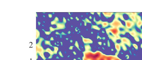
Remote Sens. 2019, 11, 533 9 of 15
over the span of a single pulse when employing phaseless reconstruction. This can offer a significant
advantage when long integration times are required.
2.2.2. Multiple Receivers
The previous results treated the case of a single receiver that measured the combined backscatter
resulting from all transmitting elements (MISO system). Building upon other RCI studies, we have
examined the advantages of implementing incoherent processing techniques, derived from optical
ghost imaging, in a microwave SAR setting. In this section, we investigate the extension of RCI to a
MIMO system through a comparison of imaging results. We employ the same geometry as that shown
in Figure 1, though allow multiple receivers to reside in the array. In the following MIMO simulations,
we simply designate each array element to be a transceiver, so that K = N = 40.
To accommodate MIMO acquisition in complex RCI, we modify the reconstruction operation to
sum the temporal correlation over all received signals:
K Z
Gc (~r ) = ∑ ∗
sre f ,k (~r, t ) s Rk ( t ) dt. (15)
k =1 t
The corresponding matrix operation can be achieved by concatenating the reference fields
corresponding to each receiver along the row direction in the H matrix of Equation (11), and including
the corresponding measurements in the s vector. Phaseless RCI can be approached similarly:
K Z Z Z
G pl (~r ) = ∑ t
2
|sre f ,k (~r, t)| |s Rk (t)| dt − κ 2
t
2
|sre f ,k (~r, t)| dt
t0
0 2
|s Rk (t )| dt . 0
(16)
k =1
This expression can be simplified by observing the equivalent frequency-domain correlation,
performed over the operating bandwidth and slow time interval:
K Z Z
G pl (~r ) = ∑ ts f
|Sre f ,k (~r, f , ts )|2 |SRk ( f , ts )|2 d f dts
k =1 (17)
Z Z Z Z
0 0 0
−κ 2
|Sre f ,k (~r, f , ts )| d f dts |SRk ( f , ts )| d f 2
dt0s
ts f t0s f0
for κ 0 = ( d f dts )−1 , and noting
R R
ts f
N
j2π f
exp −
|~r −~r Tn (ts )| + |~r Rk (ts ) −~r |
|Sre f ,k (~r, f , ts )| = | ∑ Sn ( f , ts )
2 c
|2
n =1
|~
r −~ r Tn (ts )||~r Rk (ts ) −~r |
(18)
N
j2π f
exp − c |~r −~r Tn (ts )| 2
= | ∑ Sn ( f , t s ) |
n =1
|~r −~r Tn (ts )||~r Rk (ts ) −~r |
Finally, making the approximation that |~r Rk (ts ) −~r | is nearly constant over the constellation,
the phaseless RCI image can be calculated, neglecting constant amplitude terms, as
N
j2π f K
Z Z
exp − c |~r −~r Tn (ts )| 2
G pl (~r ) = | ∑ Sn ( f , t s ) | ∑ |SRk ( f , ts )| d f dts −
2
ts f n =1
|~r −~r Tn (ts )| k =1
j2π f (19)
N Z Z K
Z Z
exp − c |~r −~r Tn (ts )| 2
κ 0
| ∑ Sn ( f , t s ) | d f dts ∑ |SRk ( f 0 , ts )|2 d f 0 dt0s ,
t s f n =1 |~r −~r Tn (ts )| t0s f 0 k =1
That is, we can simply sum the scattered intensities over the receiving aperture and use this
summed intensity in the reconstruction. This correlation operation is equivalent to that employed
in typical incoherent, optical ghost imaging, where spatial averaging of the scattered signal is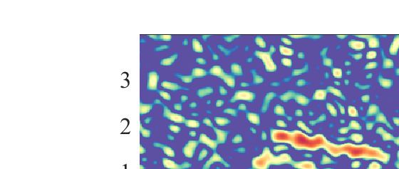
Remote Sens. 2019, 11, 533                                                                                      10 of 15

performed by an optically large bucket detector [35]. In this way, we achieve a microwave equivalent
to intensity-averaging bucket detection, with the result that we can realize incoherent SAR imaging in
which the measured intensities are related linearly to the squared magnitude of the scattering density
|σ(~r )|2 . We see that the correlation is taken with respect to a new set of reference fields consisting of
the intensities of the transmitted fields at the scene locations. Just as phaseless MISO RCI required no
phase synchronization between the transmitters and receiver, the transmitters in phaseless MIMO RCI
need not be phase synchronized with the collection of receivers. Moreover, no phase synchronization
is required between receivers, as the signals are processed incoherently.
       Figure 5 highlights the improved resolving capabilities inherent to MIMO signal acquisition. In
complex RCI, this results from the broadening of the coherent imaging system transfer function through
the convolution of the transmitting aperture’s Fourier domain coverage with that of the receiving
aperture [36,38,43]. Phaseless MIMO RCI, through incoherent processing as in Equation (19), achieves a
similar resolution enhancement. Specifically, it has been shown [35] that in the limit of an infinitely large
receiving aperture (approximately achieved as we increase K), the imaging process becomes incoherent,
so that the point spread function is the squared magnitude of that of a system employing a single point
receiver. In this case, the incoherent transfer function is given by the autocorrelation of the transmitting
aperture’s Fourier domain coverage, leading to a doubling of the transverse support in the spatial
frequency domain [36,44]. Figure 5a,b demonstrates complex and phaseless RCI reconstructions of
two closely-spaced, sub-resolution points using signals gathered with a single receiver (MISO). Clearly,
the distinct points are not resolvable under such a configuration. The case of MIMO acquisition with
complex, coherent reconstruction is shown in Figure 5c, and with phaseless, incoherent reconstruction
in Figure 5d. These images reveal the expected resolution improvement as the two points are now
distinguishable. This transition is further emphasized in Figure 5e, where cross-sections along the y
direction are plotted for MISO and MIMO, complex and phaseless reconstruction.

              (a)                (b)

                                                        (e)

                                                          1                                    MISO Complex
                                                                                               MISO Phaseless
                                                                                               MIMO Complex
                                                        0.8                                    MIMO Phaseless

                                                        0.6
              (c)                (d)
                                                        0.4

                                                        0.2

                                                          0
                                                              -1.5   -1   -0.5     0     0.5       1      1.5
                                                                                 y (m)

      Figure 5. Image of two closely-spaced point targets reconstructed using (a) complex MISO RCI,
      (b) phaseless MISO RCI, (c) complex MIMO RCI, and (d) phaseless MIMO RCI. (e) y cross-sections of
      two closely-spaced points reconstructed with complex and phaseless, MISO and MIMO RCI.

     Figure 6 compares the imaging performance for the above cases of complex and phaseless,
MISO and MIMO RCI. The simulated dataset consists of 50 pulses transmitted at equispaced positions
as the random constellation moves 40 m in the z direction. The scattered signals were received either
by a single (MISO) receiver or by all (MIMO) transceivers. A noiseless scenario is considered here to
compare the various reconstruction methods. Here, in lieu of the correlation operations described
above, reconstruction of the extended airplane target is achieved by applying the pseudoinverse of
the respective measurement matrices to the received datasets [45]. Figure 6a,b depict the results for
complex and phaseless MISO RCI, respectively. The qualitative target shape is reconstructed well by
complex RCI, whereas the target is nearly indistinguishable in phaseless RCI with a single receiver.
Remote Sens. 2019, 11, 533 11 of 15
MIMO acquisition results shown in Figure 6c,d illustrate improved fidelity and resolution under
complex reconstruction, and drastically improved image quality for phaseless reconstruction. Indeed,
since the intensity averaging performed with phaseless MIMO acquisition essentially linearizes the
problem as the system becomes incoherent, pseudoinversion applied to the measured intensities is
further justified.
Figure 6. Example RCI images of an extended airplane target using a (a) complex MISO, (b) phaseless
MISO, (c) complex MIMO, and (d) phaseless MIMO configuration.
The improved image fidelity observed in Figure 6c,d follows in part simply from the K-fold
increase in the number of measurements as the number of receivers increases from 1 to K. For the case
of complex correlation, the computational cost thus increases by a factor of K. In contrast, utilizing the
approximate phaseless, MIMO correlation given in Equation (19) incurs no additional computational
cost beyond the extra step of averaging the received signals. As the size of the region of interest grows
in practical scenarios, these savings can become increasingly advantageous.
In addition to increased computational requirements, larger regions of interest will necessitate
more measurements and transmitter modules to achieve satisfactory image quality, as mentioned
previously. Since this will inevitably be the case in practice, we briefly consider two known
reconstruction approaches that can further alleviate data size and array density requirements. The first,
called gradient ghost imaging (GGI), reduces the number of required measurements by directly
reconstructing the edges or gradient of a target [46]. For a given set of measured signals, this improves
the image SNR by reducing the effective size of the target [19,47]. Signal acquisition entails leveraging
motion of the constellation to probe the region of interest with two sets of measurement patterns that
are related simply by a transverse shift. A set of M patterns paired with M identical, but shifted,
patterns thus results in a total of 2M measurements. For each pair of shifted patterns, the difference in
the measured intensities can be computed, and this set of difference measurements correlated with one
of the set of M patterns to obtain a gradient image. Figure 7a,b compare this acquisition/reconstruction
approach to that of phaseless RCI for a 4 m by 4 m scene. For these results, signals were taken as the
random constellation moved 40 m along the z direction. At each of 25 equispaced positions along the
trajectory, a modulated pulse was transmitted and received by each element of the MIMO array. Then,
at a distance of 13 cm from these positions, an identical pulse was transmitted and received, resulting
in the interrogation of the scene with a shifted intensity pattern. Figure 7a depicts an image obtained
through phaseless RCI processing using pseudoinversion of the phaseless dataset. In this case, distinct
pulses were transmitted at each of the 50 total positions, for 2M unique measurements. GGI processing
of the target, shown in Figure 7b, achieves a gradient image with noticeably improved SNR.Remote Sens. 2019, 11, 533 12 of 15
An additional approach that can diminish artifacts resulting from reduced datasets and sparse
arrays is compressive reconstruction [39,48–51]. Figure 7c,d illustrate the results of applying TwIST [52]
to the datasets described for Figure 7a,b. An l1 regularizer was used to obtain these results, and the
solution was assumed sparse in the pixel basis. Both the phaseless RCI and gradient images are more
clearly distinguished using compressive reconstruction, with significant reduction in background
noise. We note that since the gradient image will in general be more sparse in the pixel basis than its
corresponding RCI result, GGI paired with compressive reconstruction may be a powerful combination
for alleviating measurement and sampling requirements.
(a) (b)
(c) (d)
Figure 7. Example phaseless MIMO RCI images of a pentagon structure using (a) pseudoinversion,
(b) GGI pseudoinversion, (c) TwIST, and (d) TwIST applied to GGI data.
3. Discussion
In this paper, we have extended the formulation of RCI to a fully MIMO configuration.
Although we explored details of the algorithm in the context of airborne SAR, the results are readily
extended to ground-based and spaceborne MIMO radar platforms. We also introduced phaseless
microwave RCI as an incoherent processing alternative, with the potential for reduced sensitivity
and synchronization requirements. We showed that despite the different approaches to processing
the complex and phaseless datasets, both achieved similar performance improvements under MIMO
acquisition in terms of image quality and resolution. Though coherent processing with complex data
generally requires fewer measurements for satisfactory imaging, we have seen that phaseless RCI offers
advantages through reduced synchronization demands between transmitting and receiving elements,
robustness to phase error on the receive path, reduced computational demands, and compatibility with
advanced reconstruction techniques such as gradient ghost imaging. Noiseless data was considered
in all cases in order to isolate the effects of different modalities on the resulting reconstructions.
While imaging performance will inevitably degrade with noise as in any other system, we point
out two advantages inherent to the MIMO RCI scheme. The first is that the acquisition approach of
simultaneous illumination by N transmitters naturally yields a signal-to-noise ratio improvement,
termed the Fellgett advantage [53], that is a well-known benefit of any multiplexing imaging system.
The second is that the summing of the scattered intensities over K receivers in the phaseless MIMO
RCI implementation will result in signal averaging which yields an improved signal-to-noise ratioRemote Sens. 2019, 11, 533 13 of 15
for each data point. These qualities can make MIMO RCI particularly robust to noise. Studies on the
effect of noise and other implementation specifics such as misalignment on MIMO RCI SAR will be an
interesting future direction of this work. As mentioned previously, our studies restricted the region of
interest due to computational limitations. In practice, the antenna beamwidth and resulting spot size
will determine the effective region of interest, which will necessitate longer measurement times and
larger datasets. The trends reported here may dictate which strategies become most advantageous
under such conditions, depending on dwell time and computational constraints. Finally, we have
examined only two candidate methods for reconstructing from undersampled datasets. Improved
performance can undoubtedly be achieved by employing a more appropriate sparse representation
basis [39], though in practice this choice may depend on the targets of interest.
4. Conclusions
In this work we have generalized microwave RCI to accommodate MIMO acquisition scenarios
with multiple transmitters and receivers. Whereas previous works have demonstrated coherent
processing with perfectly synchronized array elements and complex data, we have introduced and
examined incoherent RCI processing with phaseless data, for which synchronization requirements
are relaxed. In addition, we have shown that incoherent RCI exhibits reduced sensitivity to phase
error and lower computational complexity in a MIMO setting. We also showed that both coherent and
incoherent RCI processing can benefit from MIMO operation in terms of image quality and resolution.
Finally, we have demonstrated two related reconstruction methods that can be employed to further
improve performance in undersampled conditions. These considerations can be important when
evaluating trade-offs in a practical MIMO system.
Author Contributions: A.V.D. and M.F.I. conceived and designed the simulations; A.V.D. performed the
simulations and analyzed the data; A.V.D., M.F.I. and D.R.S. wrote the paper.
Funding: This material is based upon work supported by the Air Force Office of Scientific Research under award
number FA9550-12-1-0491 and FA9550-18-1-0187.
Conflicts of Interest: The authors declare no conflict of interest. The founding sponsors had no role in the design
of the study; in the collection, analyses, or interpretation of data; in the writing of the manuscript, and in the
decision to publish the results.
Abbreviations
The following abbreviations are used in this manuscript:
RCI Radar Coincidence Imaging
MIMO Multiple-Input Multiple-Output
MISO Multiple-Input Single-Output
SIMO Single-Input Multiple-Output
SAR Synthetic Aperture Radar
UAV Unmanned Aerial Vehicle
SVD Singular Value Decomposition
GGI Gradient Ghost Imaging
References
1. Li, D.; Li, X.; Qin, Y.; Cheng, Y.; Wang, H. Radar coincidence imaging: An instantaneous imaging technique
with stochastic signals. IEEE Trans. Geosci. Remote Sens. 2014, 52, 2261–2277.
2. Zhu, S.; Zhang, A.; Xu, Z.; Dong, X. Radar coincidence imaging with random microwave source.
IEEE Antennas Wirel. Propag. Lett. 2015, 14, 1239–1242. [CrossRef]
3. Li, D.; Li, X.; Cheng, Y.; Qin, Y.L.; Wang, H. Three dimensional radar coincidence imaging. Prog. Electromagn.
Res. M 2013, 33, 223–238. [CrossRef]
4. Cheng, Y.; Zhou, X.; Xu, X.; Qin, Y.; Wang, H. Radar coincidence imaging with stochastic frequency
modulated array. IEEE J. Sel. Top. Signal Process. 2017, 11, 414–427. [CrossRef]Remote Sens. 2019, 11, 533 14 of 15
5. Zhu, S.; Dong, X.; Zhang, M.; Lu, R.; Li, J.; Chen, X.; Zhang, A. A Super-Resolution Computational
Coincidence Imaging Method Based on SIMO Radar System. IEEE Geosci. Remote Sens. Lett. 2017,
14, 2265–2269. [CrossRef]
6. Soumekh, M. Synthetic Aperture Radar Signal Processing; Wiley: New York, NY, USA, 1999; Volume 7.
7. Bliss, D.; Forsythe, K. Multiple-input multiple-output (MIMO) radar and imaging: Degrees of freedom
and resolution. In Proceedings of the IEEE Thirty-Seventh Asilomar Conference on Signals, Systems and
Computers, Pacific Grove, CA, USA, 9–12 November 2003; Volume 1, pp. 54–59.
8. Haimovich, A.M.; Blum, R.S.; Cimini, L.J. MIMO radar with widely separated antennas. IEEE Signal
Process. Mag. 2008, 25, 116–129. [CrossRef]
9. Krieger, G. MIMO-SAR: Opportunities and pitfalls. IEEE Trans. Geosci. Remote Sens. 2014, 52, 2628–2645.
[CrossRef]
10. Colin, J.M. Phased array radars in France: Present and future. In Proceedings of the IEEE International
Symposium on Phased Array Systems and Technology, Boston, MA, USA, 15–18 October 1996; pp. 458–462.
11. Wang, W.Q. MIMO SAR OFDM chirp waveform diversity design with random matrix modulation.
IEEE Trans. Geosci. Remote Sens. 2015, 53, 1615–1625. [CrossRef]
12. Kim, J.H.; Younis, M.; Moreira, A.; Wiesbeck, W. Spaceborne MIMO synthetic aperture radar for multimodal
operation. IEEE Trans. Geosci. Remote Sens. 2015, 53, 2453–2466. [CrossRef]
13. Wang, W.Q. Large time-bandwidth product MIMO radar waveform design based on chirp rate diversity.
IEEE Sens. J. 2015, 15, 1027–1034. [CrossRef]
14. Yang, Y.; Blum, R.S. Phase synchronization for coherent MIMO radar: Algorithms and their analysis.
IEEE Trans. Signal Process. 2011, 59, 5538–5557. [CrossRef]
15. Godrich, H.; Haimovich, A.M.; Poor, H.V. An analysis of phase synchronization mismatch sensitivity for
coherent MIMO radar systems. In Proceedings of the 3rd IEEE International Workshop on Computational
Advances in Multi-Sensor Adaptive Processing (CAMSAP), Aruba, Dutch Antilles, The Netherlands,
13–16 December 2009; pp. 153–156.
16. Akçakaya, M.; Nehorai, A. MIMO radar detection and adaptive design under a phase synchronization
mismatch. IEEE Trans. Signal Process. 2010, 58, 4994–5005. [CrossRef]
17. López-Dekker, P.; Mallorquí, J.J.; Serra-Morales, P.; Sanz-Marcos, J. Phase synchronization and Doppler
centroid estimation in fixed receiver bistatic SAR systems. IEEE Trans. Geosci. Remote Sens. 2008,
46, 3459–3471. [CrossRef]
18. Gollub, J.; Yurduseven, O.; Trofatter, K.; Arnitz, D.; Imani, M.; Sleasman, T.; Boyarsky, M.; Rose, A.;
Pedross-Engel, A.; Odabasi, H.; et al. Large metasurface aperture for millimeter wave computational
imaging at the human-scale. Sci. Rep. 2017, 7, 42650. [CrossRef] [PubMed]
19. Gatti, A.; Bache, M.; Magatti, D.; Brambilla, E.; Ferri, F.; Lugiato, L. Coherent imaging with pseudo-thermal
incoherent light. J. Mod. Opt. 2006, 53, 739–760. [CrossRef]
20. Shapiro, J.H. Computational ghost imaging. Phys. Rev. A 2008, 78, 061802. [CrossRef]
21. Bromberg, Y.; Katz, O.; Silberberg, Y. Ghost imaging with a single detector. Phys. Rev. A 2009, 79, 053840.
[CrossRef]
22. Goodman, J.W. Statistical Optics; John Wiley & Sons: Hoboken, NJ, USA, 2015.
23. Hardy, N.D.; Shapiro, J.H. Computational ghost imaging versus imaging laser radar for three-dimensional
imaging. Phys. Rev. A 2013, 87, 023820. [CrossRef]
24. Hardy, N.D.; Shapiro, J.H. Reflective ghost imaging through turbulence. Phys. Rev. A 2011, 84, 063824.
[CrossRef]
25. Erkmen, B.I. Computational ghost imaging for remote sensing. JOSA A 2012, 29, 782–789. [CrossRef]
[PubMed]
26. Maci, S.; Minatti, G.; Casaletti, M.; Bosiljevac, M. Metasurfing: Addressing waves on impenetrable
metasurfaces. IEEE Antennas Wirel. Propag. Lett. 2011, 10, 1499–1502. [CrossRef]
27. Gonzalez-Ovejero, D.; Chahat, N.; Sauleau, R.; Chattopadhyay, G.; Maci, S.; Ettorre, M.
Additive Manufactured Metal-Only Modulated Metasurface Antennas. IEEE Trans. Antennas Propag. 2018,
66, 6106–6114. [CrossRef]
28. Sleasman, T.; F. Imani, M.; Gollub, J.N.; Smith, D.R. Dynamic metamaterial aperture for microwave imaging.
Appl. Phys. Lett. 2015, 107, 204104. [CrossRef]Remote Sens. 2019, 11, 533 15 of 15
29. Boyarsky, M.; Sleasman, T.; Pulido-Mancera, L.; Fromenteze, T.; Pedross-Engel, A.; Watts, C.M.; Imani, M.F.;
Reynolds, M.S.; Smith, D.R. Synthetic aperture radar with dynamic metasurface antennas: A conceptual
development. JOSA A 2017, 34, A22–A36. [CrossRef] [PubMed]
30. Watts, C.M.; Pedross-Engel, A.; Smith, D.R.; Reynolds, M.S. X-band SAR imaging with a liquid-crystal-based
dynamic metasurface antenna. JOSA B 2017, 34, 300–306. [CrossRef]
31. Sleasman, T.; Boyarsky, M.; Pulido-Mancera, L.; Fromenteze, T.; Imani, M.F.; Reynolds, M.S.; Smith, D.R.
Experimental Synthetic Aperture Radar with Dynamic Metasurfaces. IEEE Trans. Antennas Propag. 2017,
65, 6864–6877. [CrossRef]
32. Smith, D.R.; Yurduseven, O.; Mancera, L.P.; Bowen, P.; Kundtz, N.B. Analysis of a waveguide-fed metasurface
antenna. Phys. Rev. Appl. 2017, 8, 054048. [CrossRef]
33. Skolnik, M.I. Introduction to Radar Systems; McGraw Hill Book Co.: New York, NY, USA, 1980.
34. Diebold, A.V.; Imani, M.F.; Sleasman, T.; Smith, D.R. Phaseless computational ghost imaging at microwave
frequencies using a dynamic metasurface aperture. Appl. Opt. 2018, 57, 2142–2149. [CrossRef] [PubMed]
35. Cheng, J. Transfer functions in lensless ghost-imaging systems. Phys. Rev. A 2008, 78, 043823. [CrossRef]
36. Diebold, A.V.; Imani, M.F.; Sleasman, T.; Smith, D.R. Phaseless coherent and incoherent microwave ghost
imaging with dynamic metasurface apertures. Optica 2018, 5, 1529–1541. [CrossRef]
37. Brady, D.J. Optical Imaging and Spectroscopy; John Wiley & Sons: Hoboken, NJ, USA, 2009.
38. Marks, D.L.; Gollub, J.; Smith, D.R. Spatially resolving antenna arrays using frequency diversity. JOSA A
2016, 33, 899–912. [CrossRef] [PubMed]
39. Lustig, M.; Donoho, D.; Pauly, J.M. Sparse MRI: The application of compressed sensing for rapid MR
imaging. Magn. Reson. Med. Off. J. Int. Soc. Magn. Reson. Med. 2007, 58, 1182–1195. [CrossRef] [PubMed]
40. Lohmann, A.W.; Dorsch, R.G.; Mendlovic, D.; Zalevsky, Z.; Ferreira, C. Space—Bandwidth product of optical
signals and systems. JOSA A 1996, 13, 470–473. [CrossRef]
41. He, Q.; Blum, R.S. Cramer-Rao bound for MIMO radar target localization with phase errors. IEEE Signal
Process. Lett. 2010, 17, 83–86.
42. Krieger, G.; Moreira, A. Spaceborne bi-and multistatic SAR: Potential and challenges. IEE Proc.-Radar
Sonar Navig. 2006, 153, 184–198. [CrossRef]
43. Ahmed, S.S. Electronic Microwave Imaging with Planar Multistatic Arrays; Logos Verlag Berlin GmbH:
Berlin, Germany, 2014.
44. Goodman, J.W. Introduction to Fourier Optics; Roberts and Company Publishers: Englewood, CO, USA, 2005.
45. Zhang, C.; Guo, S.; Cao, J.; Guan, J.; Gao, F. Object reconstitution using pseudo-inverse for ghost imaging.
Opt. Express 2014, 22, 30063–30073. [CrossRef] [PubMed]
46. Liu, X.F.; Yao, X.R.; Lan, R.M.; Wang, C.; Zhai, G.J. Edge detection based on gradient ghost imaging.
Opt. Express 2015, 23, 33802–33811. [CrossRef] [PubMed]
47. Gureyev, T.; Paganin, D.; Kozlov, A.; Nesterets, Y.I.; Quiney, H. Complementary aspects of spatial resolution
and signal-to-noise ratio in computational imaging. Phys. Rev. A 2018, 97, 053819. [CrossRef]
48. Katz, O.; Bromberg, Y.; Silberberg, Y. Compressive ghost imaging. Appl. Phys. Lett. 2009, 95, 131110.
[CrossRef]
49. Eldar, Y.C.; Kutyniok, G. Compressed Sensing: Theory and Applications; Cambridge University Press:
Cambridge, UK, 2012.
50. Potter, L.C.; Ertin, E.; Parker, J.T.; Cetin, M. Sparsity and compressed sensing in radar imaging. Proc. IEEE
2010, 98, 1006–1020. [CrossRef]
51. Cetin, M.; Stojanovic, I.; Onhon, O.; Varshney, K.; Samadi, S.; Karl, W.C.; Willsky, A.S.
Sparsity-driven synthetic aperture radar imaging: Reconstruction, autofocusing, moving targets,
and compressed sensing. IEEE Signal Process. Mag. 2014, 31, 27–40. [CrossRef]
52. Bioucas-Dias, J.M.; Figueiredo, M.A. A new TwIST: Two-step iterative shrinkage/thresholding algorithms for
image restoration. IEEE Trans. Image Process. 2007, 16, 2992–3004. [CrossRef] [PubMed]
53. Gehm, M.E.; McCain, S.T.; Pitsianis, N.P.; Brady, D.J.; Potuluri, P.; Sullivan, M.E. Static two-dimensional
aperture coding for multimodal, multiplex spectroscopy. Appl. Opt. 2006, 45, 2965–2974. [CrossRef] [PubMed]
c 2019 by the authors. Licensee MDPI, Basel, Switzerland. This article is an open access
article distributed under the terms and conditions of the Creative Commons Attribution
(CC BY) license (http://creativecommons.org/licenses/by/4.0/).You can also read