Signal degradation through sediments on safety-critical radar sensors
←
→
Page content transcription
If your browser does not render page correctly, please read the page content below
Adv. Radio Sci., 17, 91–100, 2019
https://doi.org/10.5194/ars-17-91-2019
© Author(s) 2019. This work is distributed under
the Creative Commons Attribution 4.0 License.

Signal degradation through sediments on
safety-critical radar sensors
Matthias G. Ehrnsperger, Uwe Siart, Michael Moosbühler, Emil Daporta, and Thomas F. Eibert
Chair of High-Frequency Engineering, Department of Electrical and Computer Engineering,
Technical University of Munich, Arcisstraße 21, 80333 Munich, Germany

Correspondence: Matthias G. Ehrnsperger (m.g.ehrnsperger@tum.de)

Received: 30 January 2019 – Revised: 19 April 2019 – Accepted: 24 April 2019 – Published: 19 September 2019

Abstract. This paper focusses on a transmission line (TL)         at least one radar system. For these radar systems, mostly
based model which allows to investigate the impact of multi-      two frequencies are utilised: 24 GHz for short range radar
layered obstructions in the propagating path of a radar signal    (SRR) and 77 GHz for long range radar (LRR). Another fre-
at different distances and in combination with disturbances.      quency is already making its way into the automotive sector:
Those disturbances can be water, snow, ice, and foliage at dif-   5.8 GHz. Especially safety and monitoring applications are
ferent densities, temperatures, positions, with a given thick-    adapting the emerging C-band systems. The most promising
ness and layer combination. For the evaluation of the de-         advantages of 5.8 GHz are material penetration capabilities,
tectability of objects, the impulse response of the system can    reduced environmental impairment due to water, and – most
be obtained. Investigations employing state-of-the-art radar      important – low-cost availability. The main differences be-
hardware confirm the consistency of theoretical and exper-        tween the three frequencies (5.8, 24, and 77 GHz) are not
imental results for 24 and 77 GHz. The analysis in this pa-       only the associated regulations, but also their fundamentally
per supports testing the specifications for radar systems, be-    different behaviour in varying environments. Especially the
fore carrier frequency and antenna layout are finally decided.    signal attenuation due to absorption, reflection, and interfer-
Thereby, the radar system parameters can be adjusted toward       ence is highly frequency-dependent. What matters the most
employed carrier frequency, bandwidth, required sensitivity,      in the automotive and safety sector is the resiliency of a sys-
antenna and amplifier gain. Since automotive standards de-        tem, so that reliable operation can be guaranteed at any time.
fine operational environmental conditions such as temper-         For arising radar applications in the automotive and safety
ature, rain rate, and layer thickness, these parameters can       field, protective sensors for people and machinery are often
be included and adapted. A novel optimisation methodol-           subject to external installation and, hence, also to pollution,
ogy for radomes is presented which allows to boost the dy-        icing, and wetness. Especially critical safety systems must
namic range by almost 6 dB with presence of a worst-case          not be operationally affected in any way but secure safety at
cover layer of water. The findings can be utilised to prop-       all times. Hence, adverse environmental influences should be
erly design radar systems for automotive applications in au-      assessed beforehand, to ensure a sufficiently designed radar
tonomous driving, in which other vulnerable road users have       system.
to be protected under all circumstances.                             Radar sensors are advantageous for the recognition and
                                                                  detection of moving or static objects – most notably living
                                                                  objects – within a predefined vicinity, area, or space. Usu-
                                                                  ally radar systems are assembled in a locally protected en-
1   Introduction                                                  vironment to avoid signal debasing sediments. However, ex-
                                                                  ternally installed safety-critical radar-based sensors in disad-
During the last decade radar systems have experienced a re-       vantageous assembly positions are becoming more and more
naissance with a broad field of new applications. The first       popular. For living object protection (LOP) and living object
automotive radar system was employed in the 1960s, nowa-          detection (LOD), the sensors face two major challenges: first,
days all middle class and above vehicles are equipped with

Published by Copernicus Publications on behalf of the URSI Landesausschuss in der Bundesrepublik Deutschland e.V.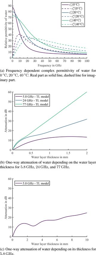
92                                                           M. G. Ehrnsperger et al.: Signal degradation through sediments

safety-critical sensor systems have – by definition – to be op-
erational at all times, to ensure maximum safety, and second,
since an external installation has to be taken into consider-
ation, the resulting environmental influences must be evalu-
ated and operationability must be self-tested. By way of illus-
trating such scenarios, Fig.1a and b show an operative radar
sensor under good weather conditions (Fig. 1a), which may
fail under different weather conditions such as rain (Fig. 1b).
   As a matter of fact, the detection of an object can only be
successful if a signal is received. For this purpose, radomes
are generally employed to protect the system. These radomes
shall not affect the antenna characteristics nor the transceived
signal in any way. Depending on the system, generally a sig-
nal is transmitted and the reflection of objects within the
propagation path of the electromagnetic wave is processed.
The received signals must be sufficiently strong to be em-
ployable. The radar equation,

                 λ2      σ    1
Pr = Pt Gt Gr                                               (1)
                (4π )3 Rt2 Rr2 LA
is helpful to estimate the received signal power. Hereby, Pr
is the power of the received signal, Pt is the power of the
transmitted signal, Gt and Gr are the gains of the transmit-
ter and receiver, respectively, λ is the free-space wavelength,
σ is the radar cross section (RCS) of the object, Rt and Rr
are the distances from the transmitter and receiver to the ob-
ject, respectively. For a monostatic radar system, where the
transmitted and received signal both are transferred by the
same antenna, the equation simplifies with Rt = Rr = R, and
Gt = Gr = G. The last term LA represents the general losses
of the system. Those can result due to all sorts of geomet-
rical, system, and climatic influences. Since externally in-
stalled radar systems are mainly affected by weather events,
in the following, the focus to evaluate LA is based on cli-
matic influences. The signal-to-noise ratio (SNR) describes
how well a signal can be distinguished from noise. If LA in-
creases as a result of sediments or the like, the SNR = Pr /N
decreases, whereby N represents the overall noise level. As
the SNR decreases, so does the probability of a successful
detection. In consequence the false alert rate increases which     Figure 1. Visualisation of a safety-critical radar system that is
significantly affects the system performance and may lead to       mounted in a disadvantageous manner, hereby flush mounted in the
a raised customer frustration and endangerment level.              ground. The sensor is exposed to environmental influences, which
                                                                   are schematically represented by the water layer. The size of the
                                                                   radar lobes schematically indicates the signal strength and therefore
2    Proposed TL-based model                                       the detection probability. The monitor symbolises a general evalua-
                                                                   tion unit which handles the received signals and displays the result,
In order to simulate an electromagnetic wave propagating           whether or not an object is detected.
through space with obstacles and discontinuities, usually full
wave solvers are utilised. For reasonably accurate results of
the full wave solution, even a small volume requires a con-        not exist in reality and are of no interest, hence, an obstacle
siderable processing power. As a trade-off of the required         within the model consists of N individual material layers.
computational power and time, as well as the accuracy of           The parameters of each layer are the relative electric permit-
results, the obstacles are approximated as infinitely extended     tivity (εr,n ) and the relative electric permeability (µr,n ), the
homogeneous layers that consist of the individual obstacle         geometrical parameter is the thickness (dn ). This layer-based
material, as illustrated in Fig. 2a. Single obstacle layers do     obstacle model is then transformed into a transmission line

Adv. Radio Sci., 17, 91–100, 2019                                                             www.adv-radio-sci.net/17/91/2019/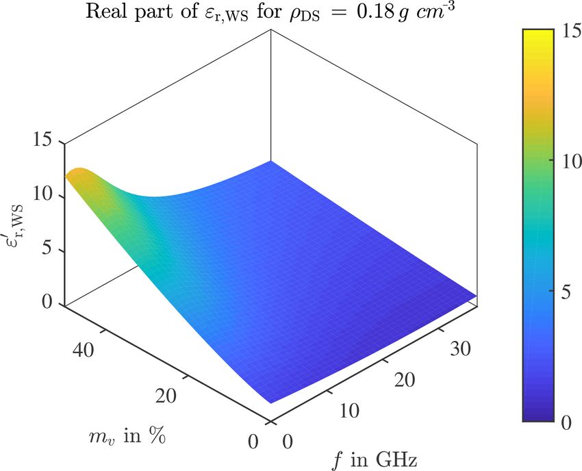
M. G. Ehrnsperger et al.: Signal degradation through sediments 93
based equivalent circuit. Hereby, each one of the layers is where the temperature is defined from about 0 to 40 ◦ C. The
transformed into an equivalent two-port, see Fig. 2b. In con- remaining parameters are calculated as
sequence, not the E- and H-fields are calculated, instead, the
model relies on voltages and currents. The model is based
on normal plane wave propagation only, without refraction, ε∞ = 0.066 εs (T ) (5)
2
oblique incidence, scattering, and polarisation effects. The fd = 20.27 + 146.5 2(T ) + 314 2(T ) in GHz. (6)
fundamental basis is provided by the impedance concept of
Schelkunoff (1951).
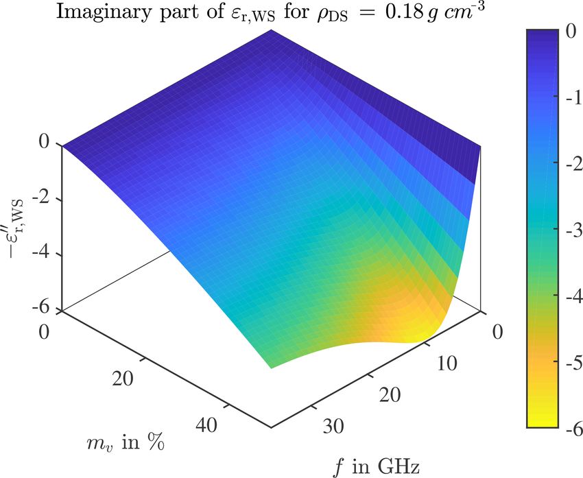
2.1 Expectable climatic and external impacts Even though such data is available in the given references,
the complex permittivity of water at various temperatures can
Based on empirical investigations, the expectable climatic be observed in Fig. 4a. Hereby, the solid line represents the
and external influences are: liquid water, as closed or contin- real part of εr , the dashed line the imaginary part. The val-
uous water layers with and without interruptions, individual ues have been printed for three different temperatures: 0,
drops, and condensation; dry or wet snow; fully-frozen ice 20, 40 ◦ C. Upon closer inspection of the imaginary part, it
layers, crystallised local spots; dry or wet foliage layers or becomes obvious that the temperature has a significant im-
individual leaves; moist or wet dirt, dust, and sedimentation pact on the position of the maximum. Over the 40 ◦ C tem-
layers. perature shift, the resonance frequency spreads over more
In general, when a signal is transmitted towards an ob- than 20 GHz. This result substantiates the large impact of
stacle, reflection, absorption, and interference attenuate the the temperature. In Fig. 4b, the one-way attenuation in dB
power that penetrates the obstacle itself (Fig. 3a). The elec- of a homogeneous water layer is plotted for thicknesses up
tromagnetic power of a wave is partially reflected at the ob- to 2 mm at 15 ◦ C. Hereby, the three frequencies of interest
stacle boundaries (Fig. 3b), partially absorbed (Fig. 3c), and are shown, 5.8, 24, and 77 GHz. The aforementioned effect
affected by multi-path propagation and interference (Fig. 3d). of interference can be nicely observed for the 5.8 GHz graph,
These effects are also taken into consideration within the since the attenuation first increases, but then, for an increased
layer based model as well as the equivalent transmission line thickness of the water layer begins to decrease. Therefore, in
(TL) model. Fig. 4c the one-way attenuation for 5.8 GHz is plotted for
a water layer thickness of up to 10 mm. Here, the effect of
2.2 Electromagnetic material characteristics interference is even more evident. For 24 and 77 GHz the
attenuation graphs show a linear tendency starting at com-
The quality of a model is highly dependent on the underlying paratively low water layer thicknesses, yet, for 5.8 GHz the
data. The data for the aforementioned expectable climatic in- effects of interference are more dominant so that a linear ap-
fluences (water, snow, ice, foliage, dirt) has been investigated proximation is only applicable for a thicker layer. To employ
theoretically and partially verified by measurements. In the valid approximations of the attenuation graphs, the equations
following the datasets of each medium are presented. of Table 1 can be employed for increased layer thickness val-
2.2.1 Electromagnetic properties of water ues. In Fig. 5 the one-way attenuation versus the frequency
is shown. The three frequencies of interest are highlighted
The implementation of the complex permittivity of water is with its corresponding attenuation offset, which is part of the
based on the model of Liebe et al. (1991). Hereby, assuming a equations of Table 1. To further illustrate the vast influence
time convention ej ωt the complex permittivity is represented of the temperature, the dashed lines in Fig. 5 indicate the
by scope of the attenuation values. Upon further investigation, it
can be observed that the higher the frequency, the larger the
εs (T ) − ε∞ effect of the temperature on the attenuation.
εr,W = + ε∞ , (2)
1 + jf/fd (T )
where the subscript “W” indicates water. The parameters 2.2.2 Electromagnetic properties of ice
are the static relative permittivity εs , the asymptotic relative
permittivity for very high frequencies ε∞ , and the resonant The dielectric behaviour of ice differs significantly from that
frequency of the molecular vibration fd . εs is temperature- of water. If water turns into ice, the dipole molecules are
dependent according to bound in a solid lattice structure, so that the reorientation
εs (T ) = 77.66 − 103.32(T ), (3) is largely prevented. Therefore, the real part and the imag-
inary part of the complex permittivity of ice are smaller than
and its calculation is based on experimental results. The tem- of liquid water with freely polarisable molecules. A possible
perature dependency is model for the dielectric permittivity of ice is given in Arage
300 et al. (2006). This proposed model is suitable for tempera-
2(T ) = 1 − , (4) tures in the range of −40 to 0 ◦ C (Hallikainen, 2014). The
273.15 + T /◦ C
www.adv-radio-sci.net/17/91/2019/ Adv. Radio Sci., 17, 91–100, 2019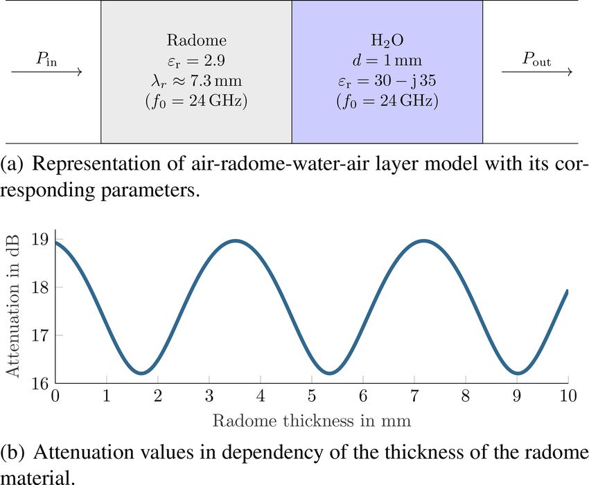
94                                                              M. G. Ehrnsperger et al.: Signal degradation through sediments

Figure 2. Comparison of the equivalent models.

Table 1. Linearised attenuation functions in dependence of frequency for certain thicknesses d.

                                      Frequency   Attenuation                               Thickness
                                      5.8 GHz     24.7 dB + 1.6 dB mm−1 (d − 10 mm)         d > 10 mm
                                      24 GHz      18.9 dB + 12.6 dB mm−1 (d − 1 mm)         d > 1 mm
                                      77 GHz      14.8 dB + 28.4 dB mm−1 (d − 0.4 mm)       d > 0.4 mm

                                                                        where the subscript “I” stands for ice. The individual param-
                                                                        eters are further stated as
                                                                        α = (50.4 + 62 2(T )) 10−4 e−22.12(T ) ,                   (8)
                                                                                                     2
                                                                             0.542 10−6 2(T2(T  )+1
                                                                                              )+0.0073 +
                                                                        β = 0.504 − 0.1312(T )                                     (9)
                                                                                                  10−4 .
                                                                                  2(T ) + 1
                                                                           Here, α has the unit GHz and β has the unit GHz−1 , T is
                                                                        the temperature in ◦ C for the valid range of −40 to 0 ◦ C.
                                                                        The resulting complex permittivity of ice has an approxi-
                                                                        mate constant real part of 3.15 and a small imaginary part.
Figure 3. Effects that occur if an electromagnetic wave impinges        The latter, however, may increase when ice is contaminated.
upon an obstacle.                                                       According to Shuji et al. (1993), chemical impurities can
                                                                        even occur in natural ice in the form of salts and acids.
                                                                        In Shuji et al. (1997), for example, winter-typical contami-
                                                                        nants such as sodium chloride (NaCl), nitroxyl (HNO) are
                                                                        examined in more detail. Concentrations between 10−5 and
relative permittivity of ice can be determined by                       10−3 mol dm−3 at a frequency of 5 GHz even led to a tenfold
                                                                        increase in the imaginary part of the relative dielectric per-
                                                                        mittivity. However, the values are still small. Dry ice as flat
                                                                        layers are far less critical than water. When the layer of ice

                           α                                            thaws, the resulting water layer has far more impact than the
εr,I (f ) = 3.15 − j         + βf ,                             (7)     ice itself. With ice, there is also the danger that an inhomo-
                           f

Adv. Radio Sci., 17, 91–100, 2019                                                                 www.adv-radio-sci.net/17/91/2019/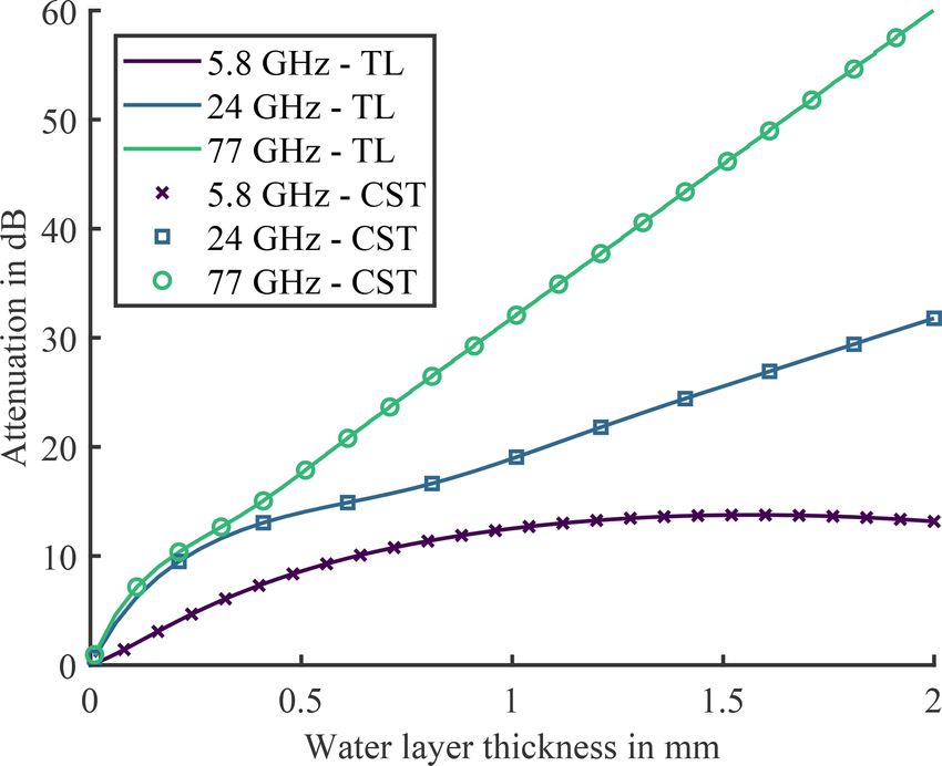
M. G. Ehrnsperger et al.: Signal degradation through sediments                                                                     95

                                                                    geneous layer thickness or a partial covering with ice could
                                                                    cause diffraction effects of the electromagnetic waves, which
                                                                    leads to distortions in the antenna characteristics (Pfeiffer,
                                                                    2010).

                                                                    2.2.3   Electromagnetic properties of snow

                                                                    Snow can be classified as dry or wet, where both consist of
                                                                    three main components: air, ice, and water. Dry snow has
                                                                    very little impact upon electromagnetic waves, since the den-
                                                                    sity is low and absorption is almost not present. The opposite
                                                                    is the case for wet snow. Wet snow has a higher density and
                                                                    consists of dry snow on the one hand, and a water volume
                                                                    fraction on the other hand. The water volume fraction with
                                                                    its freely polarisable molecules is mainly causing the attenu-
                                                                    ation of snow.

                                                                    Dry snow

                                                                    The composition of dry snow is a mixture of air and ice.
                                                                    Since the real part of the dielectric permittivity of ice corre-
                                                                    sponds to a constant, see Eq. (7), and is therefore independent
                                                                    of temperature and frequency (in the considered frequency
                                                                    range), it follows that the real part of the dielectric permittiv-
                                                                                       0
                                                                    ity of dry snow εr,DS    is also independent of the temperature
                                                                    and frequency. According to Martti et al. (1989), εr,DS  0    is a
                                                                    function that depends only on the density of the dry snow
                                                                    ρDS . As a corresponding model

                                                                                      3υi εr,I0 −1
                                                                      0
                                                                    εr,DS = 1+                          ,                      (10)
                                                                                       0 − υ ε0 − 1
                                                                                  2 + εr,I     i   r,I
                                                                                                             0 represents the real
                                                                    is considered in the following, where εr,I
                                                                    part of the dielectric permittivity of ice and corresponds to
                                                                    3.15, further υi = ρDS /ρi with ρi = 0.916. For the calcula-
                                                                    tion for the imaginary part of the permittivity of dry snow
                                                                     00      00              9υi
                                                                    εr,DS = εr,I h                        i2 ,                   (11)
                                                                                               0 (1 − υ )
                                                                                  (2 + υi ) + εr,I     i

                                                                    is employed. Since εr,I0 and ε 0
                                                                                                   r,DS are independent of the tem-
                                                                    perature and frequency, the ratio εr,DS00 /ε 00 is also charac-
                                                                                                                  r,I
                                                                    terised by this property. Due to the theoretical investigation
                                                                    of dry snow, in combination with the measurements of Martti
                                                                    et al. (1989), Ari et al. (1985), and Tiuri et al. (1984) this di-
                                                                    electric loss factor of dry snow is even lower than the already
                                                                    low loss factor of ice. Thus, the impact of dry snow on radar
                                                                    signals can be concluded as negligible.

                                                                    Wet snow

                                                                    According to Ari et al. (1985), the complex permittivity of
                                                                    wet snow is composed of two parts, namely the sum of the
Figure 4. Complex permittivity of water and the corresponding at-   permittivity of dry snow, which in turn is composed of the di-
tenuation graphs of different water layers.                         electric permittivity of air and ice, and the excess permittiv-
                                                                    ity due to liquid water in the snow, which of course depends

www.adv-radio-sci.net/17/91/2019/                                                              Adv. Radio Sci., 17, 91–100, 2019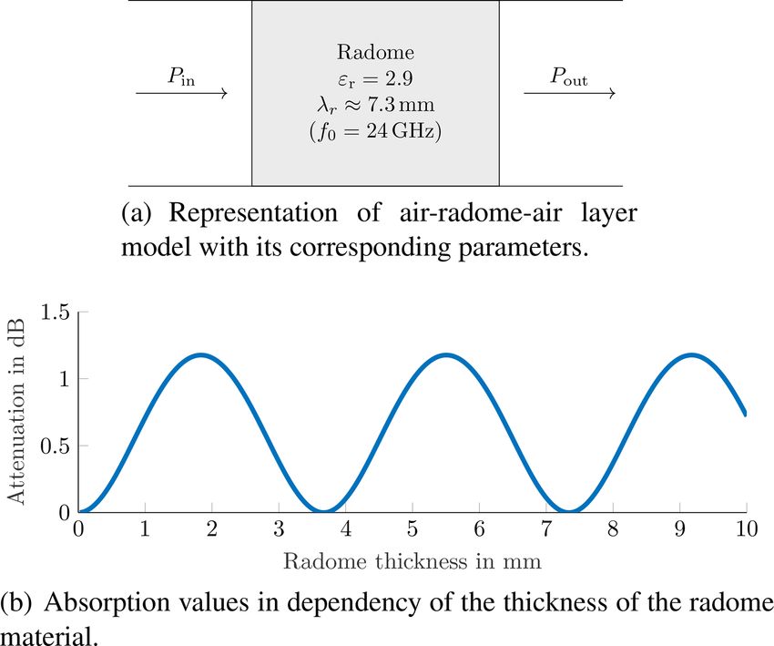
96                                                         M. G. Ehrnsperger et al.: Signal degradation through sediments

on the dielectric permittivity of water. The relative complex
permittivity of wet snow εr,WS can also be approximated
by a model, the “modified Debye-Near model” presented in
Martti et al. (1989). The model determines the dielectric per-
mittivity as

 0                B mxv
εr,WS = A+                 ,                             (12)
            1 + (f/f0 )2
 00     C (f/f0 ) mxv
εr,WS =               .                                  (13)
         1 + (f/f0 )2

   Here, f is the valid frequency (f ≤ 37 GHz), f0 is the re-
laxation frequency, mxv is the volume fraction of water (per-
centage content of liquid water). The variables A, B, C, and
x are chosen as

 x = 1.31,                                               (14)
f0 = 9.07 GHz,                                           (15)    Figure 5. One-way absorption rates in dB mm−1 of water for dif-
                                                                 ferent temperatures, with focus on 5.8, 24, and 77 GHz and the cor-
 A = 1.0 + 1.83 ρDS + 0.02 A1 m1.015
                               v     + B1 ,              (16)    responding slope for thick water layers (right value in brackets)
 B = 0.073 A1 ,                                          (17)
 C = 0.073 A2 ,                                          (18)
                               −3    2
                                                                 impact on electromagnetic waves. From this, the dielectric
A1 = 0.78 + 0.03 f − 0.58 10        f ,                  (19)    permittivity of foliage is given as
A2 = 0.97 − 0.39 f 10−2 + 0.39 10−3 f 2 ,                (20)
B1 = 0.31 − 0.05 f + 0.87 10−3 f 2 .                     (21)    εr,F = 0.522 (1 − 1.32 md ) εr,W + 0.51 + 3.84 md ,           (22)

   Different densities of dry snow components only result        where the subscript “F” indicates foliage and where the frac-
in a very small effect on the complex permittivity, a higher     tion of dry matter is valid for
density results only in a slightly higher offset of the per-
mittivity values. Accordingly, the values of the permittivity    0.16md 60.5,                                                  (23)
are primarily determined by the water content. This can also
be recognised by the fact that the larger the volume frac-       which is defined
tion of water in the snow, the greater the dielectric permit-
tivity of the water in weight, so that the permittivity of wet                       dry foliage
                                                                 md = 1 − Mg =                    .                            (24)
snow is greatly increased. The gradients of permittivities of                       fresh foliage
wet snow and water have a high qualitative consistency. This
fact allows a qualitative evaluation of the expected complex        Here, md is the dry foliage matter and Mg represents the
permittivity even for the out-of-definition frequency (Mat-      gravimetric water content. The given model is suitable for
zler et al., 1984). Snow covers in the centimetre range are      frequencies from 1 to 100 GHz. Consequently, εr,F is only
a serious limitation for a reliably functioning radar system.    dependent of the water content and the dielectric permittivity
In Fig. 6, the real part of the complex permittivity of wet      of water εr,W . εr,F is independent of the density of foliage,
snow is plotted, in Fig. 7 the corresponding imaginary part.     also the model is better suited for fresh foliage masses. In
The data represents the material constellation with density      a dry foliage mass, the water content decreases, so that the
ρDS = 0.18 g cm−3 the water volume fraction mv in % and          loss of water, the dielectric properties or the real and imag-
the frequency f in GHz.                                          inary part of the complex permittivity of leaves decrease. In
                                                                 addition, it is shown that the permittivity is very much de-
2.2.4   Electromagnetic properties of foliage                    pendent on the water content contained in the fresh foliage
                                                                 (Matzler, 1994). Studies of different models have shown that
Similar to snow, foliage can also be considered as a mix of      small volumes of air trapped in the water have a strong im-
different components. The components in this case corre-         pact on dielectric properties (Matzler, 1994). The featured
spond to high permittivity water, low to moderate permittiv-     model also includes the modelling of water, however, with-
ity organic material, and air. Matzler (1994) provides a model   out the salinity of the water in the foliage. This salinity is
for the dielectric permittivity. This was designed for foliage   about one percent, depending on the season and deciduous
of different plant species and provides information about its    species and is neglected due to the very low impact.

Adv. Radio Sci., 17, 91–100, 2019                                                          www.adv-radio-sci.net/17/91/2019/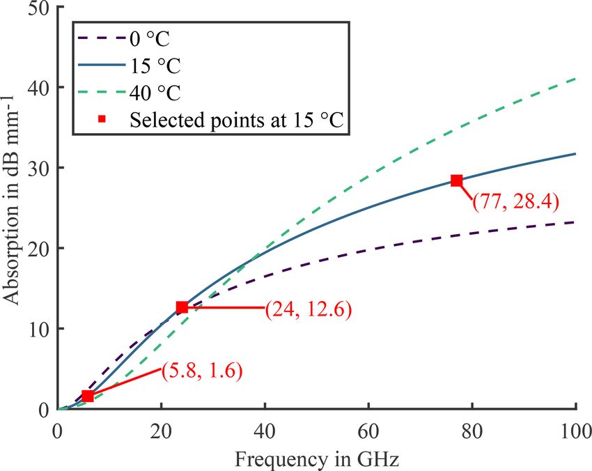
M. G. Ehrnsperger et al.: Signal degradation through sediments                                                                     97

                                                                     the dirt and it is increased, the dielectric permittivity is only
                                                                     slightly elevated. This is the result of the fact that, in addi-
                                                                     tion to the mixture, added unbound water is to some extent
                                                                     transformed into bound water. This means that the added wa-
                                                                     ter molecules are not as freely repolarisable as the free vol-
                                                                     ume of water. However, if continued to increase the percent-
                                                                     age volumetric water content, it reaches a saturation point,
                                                                     from which much more water is taken up from the ground in
                                                                     the form of bound, but the proportion of free volume water
                                                                     is increased. As a result, the dielectric permittivity increases
                                                                     faster. Soil compositions with a larger organic matter content
                                                                     can absorb more water, resulting in a later saturation point
                                                                     and thus reach a higher level of bound water. These insights
                                                                     are based on the texts given in the bibliography (Quan et al.,
                                                                     2013; Myron et al., 1985; Schmugge et al., 1978; Mironov et
                                                                     al., 2004; Ansari and Evans, 1982; Chen and Ku, 2012; Jun et
                                                                     al., 2013; Vladimir, 1994; Wolfgang and Speckmann, 2004).
                                                         0
Figure 6. Real part of complex permittivity of wet snow εr,WS for    In summary, dry soils have a real and imaginary part of the
                                                                     complex dielectric permittivity that is close to unity. These
a dry snow density ρDS = 0.18 g cm−3 depending on the water vol-
ume fraction mv in % and the frequency f in GHz.                     increase only with a volumetrically increasing water content.
                                                                     From this it can be concluded that some gravel, soil and sim-
                                                                     ilar earth compositions occurring on the concreted, paved,
                                                                     and otherwise pretreated areas do not significantly disturb the
                                                                     radar systems.

                                                                     2.3    Computational performance

                                                                     To verify the correctness and the performance of the TL
                                                                     model, the calculated results are compared to Computer Sys-
                                                                     tems Technology (CST) Microwave Studio (MWS). Hereby,
                                                                     a general purpose time domain solver, the transient solver
                                                                     which is based on the finite integration technique (FIT), of
                                                                     CST MWS has been utilised. In the simulation the air-water-
                                                                     air layer constellation has been excited with a linearly po-
                                                                     larised plane wave. What can be observed from Fig. 8 is, that
                                                                     both results from the TL model and from CST MWS agree to
                                                                     an acceptable extent. Since the test configuration is a single
                                                                     homogeneous dielectric layer that is illuminated by a plane
                                                                     wave, the comparison not only shows the correctness of the
                                                              00
Figure 7. Imaginary part of complex permittivity of wet snow εr,WS   analytical vs. the numerical solution, but also their correct
for a dry snow density ρDS = 0.18 g cm−3 depending on the water
                                                                     implementation. Comparing the required calculation power,
volume fraction mv in % and the frequency f in GHz                   taken into consideration that the TL model does not provide
                                                                     the extensive potential of CST MWS, the TL model calcu-
                                                                     lates the same result significantly faster (equal workstation
2.2.5   Electromagnetic properties of dirt                           HP-Z840 employed for calculations).

Dirt can also be considered as a four-component dielectric
mixture, which is composed of soil solids, air, bulk water           3     Radome optimisation with water layer
(free, unbound earth water) and bound water (Myron et al.,
1985). Jun et al. (2013) has created a model which takes             According to Fig. 1, a safety-critical radar sensor system is
into account a more precise composition of soil solids and           taken into consideration in the following. The surveillance
subdivides these into clay, silt and sand, with the dielectric       system monitors a hazardous area, which is unproblematic
permittivity of the soil dependent on the percentage of or-          under standard weather conditions. Climatic influences af-
ganic matter. However, the permittivity strongly depends on          fect the radar sensor performance due to absorption of en-
the free volume water. If a small volume of water is present in      ergy. The solution is to minimise the impact of absorbing

www.adv-radio-sci.net/17/91/2019/                                                               Adv. Radio Sci., 17, 91–100, 2019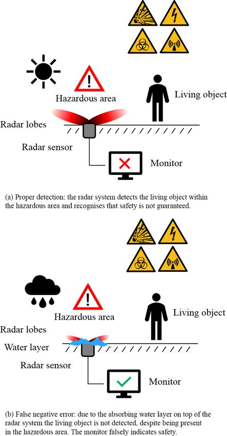
98                                                            M. G. Ehrnsperger et al.: Signal degradation through sediments

Figure 8. Result of the simulation of a commensurate layer con-
                                                                    Figure 9. Simulation setup for radome-only contemplation with the
figuration for three frequencies. The computational results of TL
                                                                    associated attenuation plot.
model and Computer Systems Technology (CST) Microwave Stu-
dio (MWS) are comparable.

                                                                       However, the result changes if a perturbing layer on top
or reflecting layers within a predefined range, all that goes       of the radome is taken into consideration. As illustrated in
beyond these limitations results in blindness of the sensor.        Fig. 10a a uniform layer of water is placed on top of the
There are several possible ways to overcome the effects of          radome material. The water layer has a constant thickness
absorbing material, the most naive solution is to increase          of 1 mm, which represents the absolute maximum for the
the transmitted power in such a way that the absorption is          given virtual application. The plot of Fig. 10b shows the total
compensated. However, as the attenuation of water can eas-          one-way attenuation versus the variation of the thickness of
ily reach high values, such an approach can only counteract         the radome material. The attenuation varies between about
insignificantly small covering layers. Especially for low-cost      16 dB and approximately 19 dB, the increased offset of the
and cost-critical systems with little dynamic range, simply         attenuation is caused by the constant uniform water layer.
increasing the transmit power is a less favourable method-          Noticeable is the fact that the positions of the minima and
ology. A more effective approach is to optimise the whole           maxima have moved. The resulting attenuation caused by
system. This means that not only the radome is optimised            the obstacle is minimised for radome thickness λ/4 and sub-
for maximum performance, but also the snow, dust, or wa-            optimal for radome thickness λ/2. The positions of optimal
ter layer that is expectable and within the absolute maximum        to suboptimal thickness have moved by about λ/4. By op-
range is taken into account.                                        timising the radome thickness for the largest possible water
   In the following a radar system at 24 GHz with a radome of       layer, the performance can be increased by almost 3 dB for
polyoxymethylene (POM) is in focus. First of all, the radome        one-way and 6 dB for return. Regarding the transferability of
is optimised in the traditional manner: in Fig. 9a the sin-         the results for the 1 mm water layer optimisation to different
gle layer radome is shown, its material parameters are the          water layer thicknesses. The local minimum of the attenua-
relative electrical permittivity of 2.9, the thickness of the       tion at radome thicknesses of about λ/4 remains, if the water
layer is now evaluated. In the context of a layer-based model,      layer thicknesses are at least as thick as stated in Table 1.
the radome represents an air-radome-air system. The corre-          Hence, for the given 24 GHz optimisation example, the same
sponding one-way attenuation of the layer composition can           results can be obtained for thicker water layers (dW > 1 mm),
be seen in Fig. 9b, where the losses are almost zero and not        however, since multi-path propagation and interference have
taken into consideration in the following. In consequence, the      higher impacts for dW < 1 mm, the position of the minimum
attenuation in Fig. 9b varies between 0 and approximately           wanders towards a optimal radome thickness of about λ/2 if
1.2 dB. The attenuation minima are located at radome thick-         the conditions of Table 1 are not met.
nesses which are multiples of λr /2, the attenuation maxima            Summarizing the result of the given example. The tradi-
where the radome thickness is an odd multiple of λr /4. Log-        tional way of optimising the radome allows to increase the
ically the radome thickness would be optimised to λr /2 –           dynamic range by about 1.2 dB, but only without a cover
hereby about 3.6 mm – to achieve maximum transmit power,            layer. The presented optimisation which considers also per-
minimised loss, and maximized performance.                          formance degrading sediment layers, allows to increase the

Adv. Radio Sci., 17, 91–100, 2019                                                            www.adv-radio-sci.net/17/91/2019/
M. G. Ehrnsperger et al.: Signal degradation through sediments 99
Figure 10. Simulation setup for radome with constant water layer
contemplation with the associated attenuation graph.
system dynamic range by almost 3 dB with presence of a
worst-case cover layer, but loses 1.2 dB without cover layer.
However, this effect is even useful for the overall system de-
sign. The realistic air-radome-water-air example would have
a total maximum attenuation of 19 dB if optimised with the
traditional approach. The radome optimisation including the
cover layer decreases the maximum attenuation to almost
16 dB. Bringing that increase of the performance in context
to the two-way attenuation of the overall system, then the dy-
namic range is increased by about 6 dB. An increase of 6 dB
allows the radar system to detect an object that is a quarter
the size (virtual size represented by the RCS), as compared
with the traditional radome optimisation.
Figure 11. Schematic illustration of the measurement setup and re-
sult plot of the measured attenuation values.
4 Experimental verification of TL model with a radar
evaluation platform
nesses. Several measurements have been carried out, the re-
To obtain relative results, the experimental setups of the sult area is plotted with its maximum and minimum values.
Fig. 11a and b have been employed. Here, the radar sys- The cubes represent the upper bound of the executed mea-
tem is positioned on the ground, looking upwards. As ref- surements, the crosses the lower bound. The solid blue line
erence object a metallic target, such as a corner reflector shows the aforementioned theoretical results including inter-
is utilised. The corner reflector is positioned on a stand at ference, reflection, and absorption effects. The measured re-
a predefined distance. The first measurement is carried out sults and the theoretical results deviate due to the complex
and the echoed power of the corner reflector is evaluated. handling and modelling of water layers, especially the thick-
The following measurements include an obstacle, the alter- ness. Since the employed radar hardware has a spatially ex-
ation in the reflected power can then be attributed accord- tended patch antenna with several channels, the uniform wa-
ingly to the obstacle. For the correct assignment of the re- ter layer must be equally distributed over the whole area. The
flected power to the metallic target, it is essential to minimise deviation originates from the surface tension of water, man-
the effects of standing waves between transceiver, obstacle, ufacturing accuracies, and the overall sum of smaller effects.
and ceiling. Hence, the modulation parameters of the radar The discrepancy at zero water layer thickness results from
system have been optimised and an application specific post- the experimental setup for introducing the water layer within
processing has been applied. Figure 11c shows the measured the reactive near-field. However, the results are reproducible
two-way attenuation of water for different water layer thick- in terms of measurement and computational accuracy.
www.adv-radio-sci.net/17/91/2019/ Adv. Radio Sci., 17, 91–100, 2019100 M. G. Ehrnsperger et al.: Signal degradation through sediments
5 Conclusions Ari, S., Ebbe, N., and Martti, T.: Mixing Formulae and Experimen-
tal Results for the Dielectric Constant of Snow, J. Glaciol., 31,
This paper was focused on the signal degradation of radar- 163–170, 1985.
based safety-critical sensors due to sediments and external Chen, H.-Y. and Ku, C.-C.: Calculation of Wave Attenuation in
influences. New applications may expose sensor systems to Sand and Dust Storms by the FDTD and Turning Bands Methods
such climatic and environmental phenomena. To assure op- at 10–100 GH, IEEE T. Antenn. Propag., 60, 2951–2960, 2012.
erationality, these signal affecting effects have to be taken Hallikainen, M.: Microwave Dielectric Properties of Materials, in
Encyclopedia of Remote Sensing, Encyclopedia of Earth Sci-
into consideration. The proposed TL-based model helps to
ences Series, New York, NY, Springer New York, 364–374, 2014.
evaluate worst-case scenarios. Measurement and simulation Jun, L., Shaojie, Z., Lingmei, J., Linna, C., and Fengmin, W.: The
results show that the model is applicable and performant. The Influence of Organic Matter on Soil Dielectric Constant at Mi-
underlying material data helps remarkably for the evaluation crowave Frequencies (0.5–40 GHz), IEEE T. Geosci. Remote,
of relevant covering layers. The practical example demon- 13–16, 2013.
strates that the proposed optimisation by employing the TL- Liebe, H. J., Hufford, G. A., and Manabe, T.: A Model for the Com-
model allows to increase the sensor performance by up to plex Permittivity of Water at Frequencies below 1 TH, Int. J. In-
6 dB under worst-case conditions. frared Milli., 12, 659–675, 1991.
Martti, T. H., Fawwaz, T. U., and Mohamed, A.: ielectric Properties
of Snow in the 3 to 37 GHz, IEEE T. Antenn. Propag., 34, 1329–
Data availability. The underlying research data can be requested 1340, 1986.
from the authors. Matzler, C.: Microwave (1–100 GHz) Dielectric Model of Leave,
IEEE T. Geosci. Remote, 32, 947–949, 1994.
Matzler, C., Aebischer, H., and Schanda, E.: Microwave Dielectric
Properties of Surface Snow, IEEE J. Oceanic Eng., 9, 366–371,
Author contributions. US and MGE conceived the presented con-
1984.
cept. ED, MM, and MG Ehrnsperger implemented the model and
Mironov, V. L., Dobson, M. C., Kaupp, V. H., Komarov, S. A., and
performed the computations. US, MM, and MGE verified the ana-
Kleshchenko, V. N.: Generalized Refractive Mixing Dielectric
lytical methods. MM and MGE carried out the experiments. MGE
Model for Moist Soils, IEEE T. Geosci. Remote, 42, 773–785,
wrote the manuscript in consultation with US and TFE. TFE super-
2004.
vised the findings of this work. All authors discussed the results and
Myron, C. D., Fawwaz,T. U., Martti, T. H., and Mohamed, A. E.-L.:
contributed to the final manuscript.
Microwave Dielectric Behaviour of Wet Soil – Part II, Dielectric
mixing model, IEEE T. Geosci. Remote, 23, 35–46, 1985.
Pfeiffer, F.: Analyse und Optimierung von Radomen für automobile
Competing interests. The authors declare that they have no conflict Radarsensoren, Doctoral Thesis, Technical University of Mu-
of interest. nich, Munich, 53 pp., 2010.
Quan, C., Jiangyuan, Z., and Ping, Z.: The Simplified Model of Soil
Dielectric Constant and Soil Moisture at the Main Frequency
Special issue statement. This article is part of the special issue Points of Microwave Band, IEEE T. Geosci. Remote, 2712–
“Kleinheubacher Berichte 2018”. It is a result of the Klein- 2715, 2013.
heubacher Tagung 2018, Miltenberg, Germany, 24–26 September Schelkunoff, S. A.: Electromagnetic Waves, Toronto, New York,
2018. London, D. Van Nostrand Company, Inc., 26 pp., 1951
Schmugge, T., Wang, J., and Williams, D.: Dielectric Constants of
Soils at Microwave Frequencies – II, NASA Technical Paper,
Financial support. This work was supported by the German Re- 1238, 1–38, 1978.
search Foundation (DFG) and the Technical University of Munich Shuji, F., Takeshi, M., Shigenori, M., and Shinji, M.: The Measure-
(TUM) in the framework of the Open Access Publishing Program. ment on the Dielectric Properties of Ice at HF, VHF and Mi-
crowave Frequencies, IEEE T. Geosci. Remote, 3, 1258–1260,
1993.
Review statement. This paper was edited by Romanus Dyczij- Shuji, F., Takeshi, M., and Shinji, M.: Dielectric Properties of Ice
Edlinger and reviewed by three anonymous referees. Containing Ionic Impurities at Microwave Frequencies, IEEE T.
Geosci. Remote, 101, 6219–6222, 1997.
Tiuri, M., Sihvola, A., Nyfors, E., and Hallikaiken, M.: The Com-
plex Dielectric Constant of Snow at Microwave Frequencies,
References IEEE J. Oceanic Eng., 9, 377–382, 1984.
Vladimir, V. T.: Model of Complex Dielectric Constant of Wet and
Ansari, A. J. and Evans, B. G. : Microwave Propagation in Sand and Frozen Soil in the 1–40 GHz Frequency Range, IEEE T. Geosci.
Dust Storms, in: IEEE Proceedings F Communications, Radar Remote, 3, 1576–1578, 1994.
and Signal Processing, 129, 315–322, 1982. Wolfgang, P. and Speckmann, H.: Radarsensoren: neue Technolo-
Arage, A., Steffens, W. M., Kuehnle, G., and Jakoby, R.: Effects of gien zur präisen Bestandsführung; T. 1, Grundlagen und Mes-
Water and Ice Layer on Automotive Radar, Robert Bosch GmbH, sung der Bodenfeuchte, Landbauforsch. Volk., 54, 73–86, 2004.
2006.
Adv. Radio Sci., 17, 91–100, 2019 www.adv-radio-sci.net/17/91/2019/You can also read