DISCO: Double Likelihood-free Inference Stochastic Control
←
→
Page content transcription
If your browser does not render page correctly, please read the page content below
DISCO: Double Likelihood-free Inference Stochastic Control
                                                        Lucas Barcelos∗,1 , Rafael Oliveira1 , Rafael Possas1 , Lionel Ott1 , and Fabio Ramos1,2

                                            Abstract— Accurate simulation of complex physical systems             On the other hand, the application of MPC to linear
                                         enables the development, testing, and certification of control        systems has been an active research area for many decades
                                         strategies before they are deployed into the real systems. As         with extensive deployments to many practical problems [1]–
                                         simulators become more advanced, the analytical tractability
                                         of the differential equations and associated numerical solvers        [3]. Notably, the most common setting for linear MPC
                                         incorporated in the simulations diminishes, making them dif-          application are tasks that involve trajectory tracking or
arXiv:2002.07379v3 [cs.RO] 26 May 2020

                                         ficult to analyse. A potential solution is the use of proba-          stabilisation. However, control tasks in reinforcement learning
                                         bilistic inference to assess the uncertainty of the simulation        are usually more complex and therefore less suitable to
                                         parameters given real observations of the system. Unfortunately       linearisation, motivating the use of non-linear models [4].
                                         the likelihood function required for inference is generally
                                         expensive to compute or totally intractable. In this paper we         Another motivation for more complex models is the ability
                                         propose to leverage the power of modern simulators and recent         to use of more expressive constraints, even if not directly
                                         techniques in Bayesian statistics for likelihood-free inference to    involved in the physical process, such as economic criteria
                                         design a control framework that is efficient and robust with          [5]. Despite its vast application in the linear case, the use of
                                         respect to the uncertainty over simulation parameters. The            MPC in non-linear systems continues to be an increasingly
                                         posterior distribution over simulation parameters is propagated
                                         through a potentially non-analytical model of the system with         active area of research in control theory [2], [3].
                                         the unscented transform, and a variant of the information                Recent work in the field has led to controllers that are able
                                         theoretical model predictive control. This approach provides          to incorporate non-linear dynamics without relying on linear
                                         a more efficient way to evaluate trajectory roll outs than            or quadratic approximations [6], [7]. However, most MPC
                                         Monte Carlo sampling, reducing the online computation bur-            controllers still do not consider uncertainty in the parameters
                                         den. Experiments show that the controller proposed attained
                                         superior performance and robustness on classical control and          of their internal simulator for future trajectories. In addition,
                                         robotics tasks when compared to models not accounting for the         estimating parameters for the system’s model usually requires
                                         uncertainty over model parameters.                                    large amounts of data from the real system, which can be
                                                                                                               infeasible for some applications. Yet, whenever the stochastic
                                                                I. I NTRODUCTION                               system uncertainties can be adequately modelled, it is more
                                                                                                               natural to explicitly take them into account in the control
                                            Robustness to model miss-specification and noisy sensor            design method itself. In Stochastic MPC, the uncertainty on
                                         measurements is a critical property for control systems               the internal system dynamics is intrinsic to the optimal control
                                         operating in complex robotics applications. The development           problem solved at every time step. This allows the controller
                                         of powerful and more realistic simulators allows practitioners        to trade-off performance and satisfaction of the constraints
                                         to analyse and verify the performance of the controller               by regulating the joint probability distribution of the system
                                         against these variables before the controller is deployed to          states and outputs [3].
                                         the real robot. In Model Predictive Control (MPC) one seeks              In this paper we make the following contributions: we
                                         to iteratively find the solution of an optimisation problem           develop a Stochastic Non-linear MPC variant which leverages
                                         for a receding finite time-horizon using an approximate               recent advancements in likelihood-free inference to estimate
                                         model of the system. When the dynamic model is given by               both the uncertainty on the simulator parameters as well
                                         complex simulators that incorporate differential equations            as to propagate it throughout the estimated trajectories. We
                                         and numerical solvers there is little hope the equations              call our method double likelihood-free inference stochastic
                                         can be reversed to reason about the parameters of the                 control, DISCO. The posterior distribution for the parameters
                                         simulation to best match the real behaviour of the system.            of the simulator is estimated by combining simulated data
                                         Furthermore, the simulator might abstract away the equations          from generative models and observations from the physical
                                         and solver from the user. Effectively, it can be interpreted as       system. Using this posterior distribution allows us to take
                                         a generative model that can be sampled from given a set of            into account the uncertainty about the system’s dynamics
                                         parameter values, but not inverted. In this paper we pose the         in the decision making process during the control task.
                                         question, can we leverage the power of simulators, treated as         We proceed to show that the Unscented Transform (UT)
                                         generative models, to design control strategies that are robust       [8] provides a computationally efficient alternative when
                                         to parameter uncertainty?                                             compared to traditional Monte Carlo approaches to propagate
                                                                                                               the uncertainty from the parameter space to the forward
                                           ∗ Corresponding author: lucas.barcelos@sydney.edu.au
                                           1                                                                   modelling of the trajectory roll outs. In short, DISCO can
                                             School of Computer Science, The University of Sydney, Australia
                                           2 NVIDIA, USA                                                       be seen as a variant of the Information Theoretical MPC (IT-
                                           Code available at: https://github.com/lubaroli/disco                MPC) control algorithm [7] that considers the uncertainty in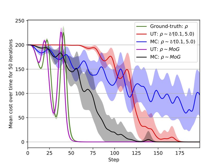
the system’s parameters in its internal trajectory simulations.   cost function to be differentiable and assures that a feasible
                                                                  solution will exist.
                    II. R ELATED WORK                                Additionally, DISCO takes advantage of the BayesSim
   The use of MPC in the control of linear systems is very        Likelihood-free Inference (LFI) framework presented in [14]
mature and has been widely studied and applied to real            to update the model uncertainty periodically. Hence, given a
systems. However, as seen in [2], Non-linear MPC (NMPC)           set of true observations after a specified episode length, we
is still an open-research question, especially for systems were   can update our knowledge of the posterior probability density
uncertainty over parameters and constraints on controls and       of parameters p(θ|x = xr ). This way our model can adapt to
state-space are considered. The most common methods for           variations in the environment, e.g. adjust friction coefficients
controlling general nonlinear systems are based on Non-linear     in case of rain, or intrinsic to the transition function, e.g.
Programming [9] and Differential Dynamic Programming              change of weight distribution. In contrast to other inference
(DDP) [10]. Both rely on approximations of dynamics               methods, such as Variational Inference or Markov Chain
and cost functions so that the online optimisation problem        Monte Carlo, where a likelihood function is needed, in LFI
becomes tractable. However, these mainstream gradient-based       we compute an approximated parametric distribution of the
MPC approaches have some shortcomings. In the DDP                 true posterior. Furthermore, BayesSim was shown to be more
method, the cost function must be smooth and it is notoriously    data efficient than other LFI methods, such as Approximate
difficult to include state constraints. Whereas with nonlinear    Bayesian Computation [14].
programming constraints may be easily accounted for, but
a common issue is what to do when no feasible solution is                                III. P RELIMINARIES
found.                                                               We consider the problem of controlling a discrete-time
   In [3], a family of Stochastic NMPC (SNMPC) methods are        stochastic system described by a non-linear set of difference
discussed. In Tube-based NMPC the objective of the control        equations of the form:
policy is to ensure that the forward trajectories will remain
inside a desirable tube centred around a given trajectory,                                xt+1 = f (xt , vt )                    (1)
however the boundary tube has to be computed offline [11].
A multi-stage NMPC approach has been suggested in which           where f is the transition function, xt ∈ Rn denotes the
the uncertainty is modelled by a scenario tree approach from      system states, and vt ∼ N (u, Σ) ∈ Rm is the control input
stochastic programming. However, the procedure quickly            at a given time t. We assume a finite time-horizon T , and that
becomes intractable, since the size of the optimisation           the control frequency is given. Note that there is no direct
problem scales exponentially with the time horizon, number        control over the variable v, but we are able to control its
of uncertainties and uncertainty levels [12].                     mean u. This assumption considers not only a multiplicative
   Although many of the methods above focus on robustness,        noise model which is common in robotics, where lower-level
they do not incorporate uncertainty over the parameters of        actuator controllers are usually present, but also an amount
the transition function. In [5], this is accounted for by using   of exploration in our control actions. As such, in practice, Σ
a SNMPC with an Unscented Kalman Filter to propagate              is a hyper-parameter of our control system that may need to
the uncertainty over the state-space. However, this method        be artificially increased.
requires an optimisation with chance constraints to be solved        More generally, we are interested in the problem where the
online and, to keep the problem feasible, the variance of         real transition function f (x, v) is approximated by a param-
the trajectories has to be artificially constrained. The most     eterised non-linear forward model f (x, v, θ), represented as
similar approach is perhaps presented in [13], where the IT-      fθ for compactness. Equation (1) may then be rewritten as:
MPC formulation is used in conjunction with a Ensemble of
                                                                                         xt+1 = fθ (xt , vt ) .                  (2)
Mixture Density Networks (E-MDN) to approximate the joint
probability distribution of states and actions. This is similar   A. Information Theoretical MPC (IT-MPC)
to our approach, however as the E-MDN tries to approximate
                                                                     Following the steps in [7], we can define a fixed length input
the joint distribution of states and actions, it needs to be
                                                                  sequence U = (u0 , . . . , uT −1 ) over a fixed control horizon
retrained entirely on new environments.
                                                                  T , onto which we apply a Receding Horizon Control strategy.
   In contrast, the variant of IT-MPC proposed in this
                                                                  This yields V = (v0 , v1 , . . . , vT −1 ) ∈ Rm×T , which is itself
paper uses the UT to propagate the uncertainty over model
                                                                  a random variable. Furthermore, let’s denote as P the joint
parameters. This reduces the dimensionality of the inference
                                                                  probability distribution and p the corresponding probability
problem and results in a controller more adept to generalise to
                                                                  density function (pdf) of the uncontrolled system (i.e. U ≡ 0).
unseen situations. Moreover, unlike the stochastic optimisation
                                                                  Likewise, Q is the joint distribution and q the corresponding
strategies, our framework is very amenable to the inclusion
                                                                  pdf for an open-loop control sequence. The optimal control
of constraints, as the control update law is based on sampled
                                                                  problem may then be be defined as:
trajectories. As shown in [7] constraints may be applied
directly to the control actions. On the other hand, we can                                                     −1
                                                                                             "               T
                                                                                                                              #
                                                                                                             X
                                                                            ∗
apply soft constraints to the state space through the cost                U = argmin EQ φ (xT ) +                 L (xt , ut ) ,  (3)
                                                                                  U ∈U
function. This is easily achieved as there is no need for the                                              t=0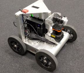
where U is the set of admissible controls, φ (xT ) is a terminal             B. Likelihood-free parameter estimation
cost function, and L (xt , ut ) is a running cost function of                   Recent advances in LFI allowed the use of probabilistic
the form:                                                                    inference to learn distributions over simulation parameters
                                   λ T −1                                    [14]. The main idea is that of approximating an intractable
                                      ut Σ ut + βtT ut ,

        L (xt , ut ) = c (xt ) +                                    (4)
                                   2                                         posterior p(θ|x = xr ) using data generated from a generative
where λ ∈ R+ is known as the inverse temperature and the                     forward model (or simulator) where trajectories are collected
affine term β allows the location of the minimum control (rest               for different simulation configurations. Therefore, one can
position) to be different from zero. Noting that the state cost              directly learn a conditional density qφ (θ|x) where parameters
may be considered independent from the                                       φ are learned through an optimisation procedure. The learned
                                          PTcontrol
                                              −1
                                                       terms, we can
define C (x0 , x1 , . . . xT ) = φ (xT )+ t=0 c (xt ). Moreover,             model usually takes the form of a mixture of Gaussians where
we define a mapping operator, H, from input sequences V                      inputs are summary statistics obtained from trajectories and
to their resulting trajectory by recursively applying fθ given               outputs are the parameters of the mixture. Q
x0 , H(V ; x0 , θ) = [x0 , fθ (x0 , v0 ), fθ (fθ (x0 , v0 ), v1 ), . . .].      The goal is to maximise the likelihood n qφ (θn |xn ). It
This leads to the following state cost function:                             has been shown in previous work [14] that qφ (θ|x) will be
                                                                             proportional to p̃(θ)
                                                                                               p(θ) p(θ|x) if the log-likelihood is optimised
              S (V ; x0 , θ) = S (V ) = C (H (V )) .                   (5)
                                                                             as follows:
   Finally, IT-MPC relies on the free-energy principle to                                               1 X
compute a lower bound for the optimal control problem and                                     L(φ) =           log qφ (θn |xn )          (11)
                                                                                                        N n
defines the form of the optimal distribution function q ∗ (V )
for which this bound is tight and achieves the optimal control               Consequently, a posterior estimate can be obtained by:
U ∗ . It can be shown that such distribution is of the form                                                 p(θ)
                    1

                               1
                                                                                         p̂(θ|x = xr ) ∝         qφ (θ|x = xr ).       (12)
            ∗
           q (V ) = ∗ exp − S(V ) p(V )                    (6)                                              p̃(θ)
                   η           λ
                   Z                                                          The conditional density qφ (θ|x) is a mixture of K Gaus-
                                   1
              η∗ =        exp − S(V ) p(V )dV,             (7)               sians,
                    R m×T          λ                                                           X
where the base distribution p(V ) has been augmented with the                       qφ (θ|x) =   Kαk (x)N (θ|µ(x)k , Σk (x)),       (13)
                                                                                              k=1
cost of the state trajectory. This results in u∗i = EQ∗ [vt ] ∀t ∈
{0, 1, . . . T − 1}. Therefore, the optimal open-loop control                where  {αk (x)}K
                                                                                            k=1 are mixing functions, {µk (x)}K
                                                                                                                              k=1 are
sequence is the expected value of control trajectories sampled               mean functions and {Σk (x)}K
                                                                                                        k=1 are covariance functions.
from the optimal distribution. As we cannot sample directly
from Q∗ , we can resort to importance sampling [15] to                                                IV. DISCO
construct an unbiased estimator of the optimal distribution,                    At its core, model-based control relies on an approximated
given the current control distribution, namely                               transition function to optimise the control actions over
                Z                 Z                                          the control horizon. In practice, this transition function is
  EQ [vt ] = q ∗ (V )vt dV = ω(V )q(V |Û , Σ)vt dV, (8)                     usually defined a priori using fundamental physical principles
                                                                             and domain knowledge, or empirically by applying system
where ω(V ) = q ∗ (V )/q(V |Û , Σ) is the importance sampling               identification techniques [16] or learning methods from data
weight. Therefore, we can switch the expectation to EQÛ ,                   [16]–[18]. Typically, these methods provide deterministic
resulting in EQÛ [ω(V )vt ]. We can then use the definition of              transition functions that do not incorporate model uncertainty
the optimal distribution w.r.t. the base measure distribution                and are invariant over time. As discussed in [6], the closed-
given in [7] to derive the optimal information-theoretic control             loop RHC offers a degree of robustness to model uncertainties,
law:                                                                         but the compounding error of poor predictions along the
                                           −1
                                                       !!
               1          1
                                         T
                                         X                                   control horizon will reduce the stability margins of the system.
                                               T −1
     ω(V ) = exp −             S(V ) + λ      ut Σ vt                        Using the methods outlined in section III, in this paper we
               η          λ              t=0                                 propose a framework to apply the IT-MPC stochastic control
         ut = EQÛ [ω(V )vt ] ,                                        (9)   formulation to problems where the parameters of the transition
where:                                                                       function fθ are unknown, but belong to a problem dependent
         Z                              T −1
                                                           !!                prior, p(θ). Furthermore, we make use of BayesSim [14] to
                   1                    X
                                                   −1                        refine our knowledge of the parameters as we interact with
   η=        exp −         S(V ) + λ           uT
                                                tΣ    vt        , dV
                   λ                    t=0
                                                                             the environment and gather new observations. The intuition
                                                            (10)             behind this approach is that, by refining our knowledge
and ut = (ût − ũt ) is the difference between the current                  of the parameters of an otherwise well-defined transition
control action ût and the minimum control ũt (adjusted by β                function, we will capitalise not only on the application domain
and usually zero). Note that in practice, for numerical stability,           knowledge, but also on the adaptability of inference-free
we multiply the  numerator and denominator of ω(V ) by a                    learning methods. Since θ represents a plausible range of
factor exp λ1 ρ , where ρ is defined as the minimum cost.                    unknown physical parameters, e.g. mass or friction coefficient,
it is straightforward to incorporate domain knowledge to this In DISCO, we refer to the formulation presented in [21] to
formulation. Alternatively, an improper uninformative prior compute sigma-points over the distribution p(θ) of parameters.
may be used when no assumptions are given. On the other The expressions to compute the sigma-points and weights for
hand, by updating our knowledge of p(θ|x = xr ) given the mean, $0m , and covariance, $0c , are presented below:
observed data, we are more likely to cope with problems p
such as covariate shift [19] and reality gap [14], [20]. The χ0 = θ χi = θ + ( (n + ν)Σθ )1≤i≤n
ν p
complete method is presented in algorithm 1. $0m = χi = θ − ( (n + ν)Σθ )n+1≤i≤2n
n+ν
A. Problem setup 1
$0 = $0m + 1 − ν 2 + ξ
c
$im = $ic =
,
2(n + ν)
Given a forward model with parameters θ and distributed
(16)
according to p(θ), trajectories can be obtained from it by
first sampling θ and generating roll outs by propagating the where ν = α2 (n + κ) − n is the primary scaling factor, κ
state-action pairs through the transition function. Although a secondary scaling (usually 0), α determines the spread
the parameters are stochastic, we assume they are invariant of the sigma points around θ, and ξ is a scalar to provide
throughout the control horizon for a given trajectory. This is an extra degree freedom. The reader is encouraged to refer
a reasonable assumption as the latent parameters are usually to [21] for details on hyperparameter selection. The sigma-
stable physical quantities and the update frequency of the points are then applied recursively to the transition function
control loop is significantly faster than their time constants. In fθ to compute the cost Sθ (V ; θ = χi ) for i ∈ {1, . . . , L}.
this situation, the optimal distribution given in (6) becomes: In practice, the sigma points on the state space are given
by γ = H(χ). To ensure the trajectory cost of each sigma-
∗ 1 1
q (V, θ) = exp − Sθ (V ) p(V |θ)p(θ), (14) point can be summarised using the UT, it is necessary to
η λ apply the same action sequence V sampled i.i.d. to all points.
where we overload the notation to emphasise the dependence Effectively, this means we need to replicate L times each
of S(V ) on the now stochastic θ. However, as V and θ are action sequence V during our update step. Finally, the mean
independent, we can drop the conditioning in p(V |θ) = p(V ). trajectory cost is given by
As a result, our control law can be expressed as: L
X
S(V ) = $im Sθ (V ; θ = γ i ), (17)
ut = EQÛ [EQθ [ωθ (V )vt ]] = EQÛ ,θ [wθ (V )vt ] , (15)
i=0
where ωθ shows the dependence on θ and we applied the and used in (9) for the control law update.
law of total expectation to get the resulting equivalence. This
means our update rule now has to sample jointly from the C. Updating the parameter prior distribution
distributions of V and θ. At each time step we are computing a new control action
ut , applying it to our environment and collecting new
B. Propagation of uncertainty over the state-space dynamics observations xrt+1 . The pairs of [ut , xrt ] represent a trajectory
If we sample sufficiently from p(V, θ), we are able τ , up to a specified time-length. This serves as input for
to reconstruct the joint distribution q(V, θ) and compute the estimate of the posterior probability of p(θ|τ ). Once
our control updates. However, we note that the increased sufficient data has been aggregated in τ , we can use the
dimensionality of the sample space requires the number method presented in [14] to refine the posterior estimate.
of samples to grow combinatorially. As such, we resort to Finally, the unscented transform requires as an input a
the unscented transform [8] as more efficient approach to mean vector θ and covariance matrix Σθ for the parameters.
propagate the uncertainty of θ throughout the state-space. Therefore, these have to be retrieved from qφ (θ|τ ), or,
In [8], the authors demonstrate how UT is able to recon- alternatively, the highest weighted Gaussian may be selected
struct an approximate Y 0 (x) of the random variable Y = if it is above a specified threshold.
g (X) resulting when an original random variable X is applied V. E XPERIMENTAL RESULTS
to a non-linear function g. The premise behind this approach
is that it should be easier to approximate a probability A. Inverted pendulum swing-up task
distribution than a arbitrary non-linear transformation. The In this task, the controller has to swing and hold a pendulum
idea is to select a set of sigma points able to capture the most upright using a torque command applied directly to the joint
important statistical properties of the prior random variable of a rigid-arm. We used the simulator in [23], and always set
X. The necessary statistical information captured by the UT the pendulum initial state to the downright position and at
is the first and second order moments of p(X). The number rest. The state cost function used was c = 50 cos(θ −1)2 + θ̇2 ,
of sigma-points needed to do this L = 2n + 1, where n is and the terminal cost function φ was set to zero. The inverse
the dimension of X. In [21], it is shown that matching the control temperature λ was set at 10 and the control authority Σ
moments of X up to the nth order implies matching the at 1. We have also defined the number of sampled trajectories
moments of Y to the same order. By using a larger number K = 500 and the control horizon T = 30. For more details
of sigma-points, skew and kurtosis can also be captured [22]. on the experiment parameters, please refer to the Appendix.Algorithm 1: DISCO
Control Hyperparameters: λ, Σ, β, c, φ;
UT Hyperparameters: ν, κ, α, ξ;
Given: fθ , p(θ), U0 , T , K, L, τ ;
Update posterior distribution;
qφ (θ|τ ) ← BayesSim(τ );
p (θ) ← qφ (θ|τ );
while task not complete do
x0 ← GetStateEstimate();
for k ← 0 to K − 1 do
Sample E k = k0 . . . kT −1 , kt ∼ N (0, Σ);
for i ← 1 to L do
θ i ← θ ∼ p(θ) (MC) or χi (UT);
x ← x0 ;
for t ← 1 to T do Fig. 1: Mean cost over time for the inverted pendulum
x ← fθ (x, vt , θ i ); experiment. Shaded area represents one standard deviation.
Sik += c(x) + λuT −1 Three models where evaluated: a standard IT-MPC with
t−1 Σ (t−1 );
end access to the true system parameters (in green); DISCO
Sik += φ(x); using unscented transform with a prior distribution over
end parameters (in red) and with an updated posterior distribution
PL
S k = i=1 $im Sik ; (in magenta); and DISCO using MC sampling with a prior
end distribution (in blue) and an updated posterior (in black).
ρ ← min(S k );
PK
η ← k=1 exp − λ1 S k − ρ ;
for k ← 1 to K do shared the same posterior distribution estimate. Once trained
and conditioned on the observed data, the resulting mixture
ωk ← η1 exp − λ1 S k − ρ ;
had a mean estimate for the length of 0.89 meter and for
end
mass 0.90 kilo. The covariance matrix was diagonal, and the
for t ← 0 to T − 1 do
PK−1 variance was 0.01 for the length estimate and 0.03 for mass.
ut += k=0 ω E k kt ; One of the components of the mixture was dominant with a
end weight of 0.979 and was used as reference for the UT.
SendToActuators(u0 ); DISCO with UT outperforms MC sampling both with
Append(τ , [x0 , u0 ]); an uninformative prior and inferred posterior. Noticeable
RollControlActions(u); also, the performance of UT with the posterior distribution
end is better than the baseline model. This is explainable by
the fact that the parameter randomisation introduced by the
sigma-points provides more information in the trajectory
The results presented in Figure 1 are the mean cost over evaluation. This way, trajectories that are borderline to a
time for 50 iterations, for a baseline case, DISCO, and Monte higher cost state captured by one of the sigma points get
Carlo sampling. Note that the oscillatory behaviour of the penalised. Effectively, UT works like an automatic calibration
cost function is expected, as the controller has insufficient of the control temperature, when the prior is broad, many
authority to balance the pendulum without the swinging action trajectories are considered in the control update average.
to increase the momentum. Conversely, when the posterior gets refined, the controller is
All models used the same hyperparameters described above, more confident to select fewer trajectories.
with the exception of the T for the case of MC sampling.
Given that we want to compare the performance of the B. Skid-steer robot
controller when using UT against MC, for the case where This section presents experimental results with a physical
MC is used, we increment the amount of trajectories sampled robot equipped with a skid-steering drive mechanism (Fig-
by the number of sigma points L used by the UT. Effectively, ure 2). We modelled the kinematics of the robot based on
for the MC controller we have K = 2500 trajectories. a modified unicycle model, which accounts for skidding
The unknown parameters in this example were the length via an additional parameter [24]. The parameters to be
of the arm and the mass of the pendulum. As a prior, we estimated via BayesSim are the robot’s wheel radius rw ,
assumed an uniform distribution between 0.1 and 5 for both axial distance aw , i.e. the distance between the wheels, and
parameters. The posterior distribution was given by a mixture the displacement of the robot’s instant centre of rotation (ICR)
of Gaussians with 5 components, trained using a reference from the robot’s centre xICR . A non-zero value on the latter
control policy. Note that in our simulations, both models affects turning by sliding the robot sideways. To estimate theparameters, the robot was driven manually around a circle
and had its trajectory data recorded. From the trajectory
data we computed cross-correlation summary statistics as
(x, y, ∆x, ∆y), which capture the centre of trajectory and
the average linear velocity. In simulation, the wheel speed
commands sent to the robot were repeated N = 1000 for
different parameter settings sampled from a uniform prior,
xICR ∼ [0, 0.5], rw ∼ [0, 0.5], aw ∼ [0.1, 0.5].
Figure 2b presents the resulting marginal estimates from
BayesSim for each parameter of the robot’s kinematic model.
For comparisons, physical measurements indicate a rw of
around 0.06 m and aw of around 0.31 m. Measuring xICR , (a) Robot (b) Marginals
however, involves a laborious process, which would require Fig. 2: Skid-steer robot and its parameter estimates
different weight measurements or many trajectories from the
physical hardware [25]. As we are only applying a relatively
simple kinematic model of the robot to explain the real
trajectories, the effects of the dynamics and ground-wheel
interactions are not accounted for. As a result, BayesSim tries
to compensate for the miss-specifications in some parameters
estimation, such as the axial distance. This explains the larger
variation in aw , and consequently xICR .
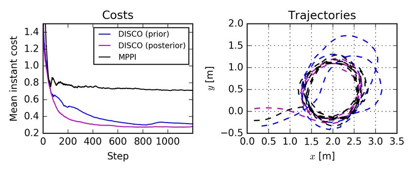
The control task was defined as following a circular path
at a constant tangential speed. Costs were set to make
p robot follow a circle of 0.75 m radius with c(xt ) =
the
Fig. 3: Results with physical robot
d2t + (st − s0 )2 , where dt represents the robot’s distance
to the edge of the circle and s0 = 0.2 m/s is a reference linear
speed. We performed experiments sampling from the uniform
prior over the parameters p(θ), sampling from the posterior the building blocks of an adaptive controller framework, more
q(θ|τ ), and using only a point estimate set to xICR = 0.12, resilient to issues arising from reality gap and covariate
rw = 0.06 and aw = 0.47, which was adjusted offline to shift. As shown in the robotic experiments, incorporating
reduce simulation error. For clarity, instead of thePnoisy raw uncertainty may lead to a more accurate assessment of the
t environment and increase the performance.
costs, we present the mean instant cost, i.e. ct = 1t i=1 c(xi )
and the executed trajectories in Figure 3. For the complete The unscented transform proved an efficient way to propa-
experiment parameters refer to the Appendix. gate uncertainty, reducing the burden of sampled trajectories.
We see that considering parameter uncertainty via DISCO When combined with the ability to impose hard-penalties on
provides significant performance improvements over the the state cost, the result is similar to a chance constraint, where
baseline IT-MPC algorithm running with a point estimate. the resulting trajectories from sigma points that violate the
Although, in term of costs, both the prior and posterior soft constraints are heavily penalised. It is worth noticing, that
estimates offer similar performance, we see the advantages this deterministic method of estimating the moments of the
of using the parameter posterior estimates in the trajectories parameter distribution allow the task of sampling actions to be
plot, where we see overshooting happening on some portions parallelised asynchronously and aggregated when computing
of the path. The latter can be explained by the prior allowing the final cost. In future work we intend to explore further
kinematic parameters candidates that are too far from the possibilities of uncertainty propagation in a principled way.
true values. Additionally, refining the posterior distribution More importantly, we showed how LFI is a powerful tool
allows the system to adapt to new configurations or drift in to refine the estimation of the posterior distribution. As the
the model parameters. Lastly, a noisier speed control explains inference is based on the same transition function fθ of the
the gap between the baseline MPPI and the DISCO methods, controller, it may compensate overly simplified models of
despite the similar performances in terms of path tracking. the environment. Therefore, we want to explore pathways to
efficiently retrain this estimate online so practical experiments
VI. C ONCLUSION with time-variant parameters may be conducted. This is a
This paper is a first step towards incorporating model crucial step towards generalisation of control policies for
uncertainty and sophisticated Bayesian inference methods autonomous robots operating under varying environments and
to stochastic model based control. We showed how un- configurations. Crucially, by combining parameter estimation
certainty over parameters may be formally incorporated and gradient-free control methods, DISCO may also be
into an stochastic non-linear MPC controller and evaluated used with black-box simulators, such as data-driven function
methods of propagating the uncertainty into trajectory roll approximators, as long as we are able to sample efficiently
outs. This extension to information theoretical MPC provides from them. This is a promising direction for future research.R EFERENCES [14] F. Ramos, R. Possas, and D. Fox, “BayesSim: Adaptive Domain
Randomization Via Probabilistic Inference for Robotics Simulators,” in
[1] L. de Oliveira and E. Camponogara, “Multi-agent model predictive Proceedings of Robotics: Science and Systems, Jun. 2019, event-place:
control of signaling split in urban traffic networks,” Transportation FreiburgimBreisgau, Germany.
Research Part C: Emerging Technologies, vol. 18, no. 1, 2010. [15] C. Andrieu, N. De Freitas, A. Doucet, and M. I. Jordan, “An
[2] D. Q. Mayne, “Model predictive control: Recent developments and introduction to MCMC for machine learning,” Machine Learning,
future promise,” Automatica, vol. 50, no. 12, pp. 2967–2986, Dec. 2003, arXiv: 1109.4435v1 ISBN: 0885-6125.
2014. [Online]. Available: http://www.sciencedirect.com/science/article/ [16] M. Simchowitz, H. Mania, S. Tu, M. I. Jordan, and B. Recht,
pii/S0005109814005160 “Learning Without Mixing: Towards A Sharp Analysis of Linear
[3] A. Mesbah, “Stochastic Model Predictive Control: An Overview and System Identification,” arXiv:1802.08334 [cs, math, stat], Feb. 2018,
Perspectives for Future Research,” IEEE Control Systems Magazine, arXiv: 1802.08334. [Online]. Available: http://arxiv.org/abs/1802.08334
vol. 36, no. 6, pp. 30–44, Dec. 2016. [17] S. Schaal, “Learning from Demonstration,” in Advances in Neural
[4] B. Recht, “A Tour of Reinforcement Learning: Tutorial,” 2018 ICML Information Processing Systems 9, M. C. Mozer, M. I. Jordan, and
Tutorial, p. 80, 2018. T. Petsche, Eds. MIT Press, 1997, pp. 1040–1046. [Online]. Available:
[5] E. Bradford and L. Imsland, “Stochastic Nonlinear Model Predictive http://papers.nips.cc/paper/1224-learning-from-demonstration.pdf
Control with State Estimation by Incorporation of the Unscented [18] P. Abbeel, A. Coates, and A. Y. Ng, “Autonomous Helicopter
Kalman Filter,” arXiv:1709.01201 [math], Sep. 2017, arXiv: Aerobatics through Apprenticeship Learning,” The International
1709.01201. [Online]. Available: http://arxiv.org/abs/1709.01201 Journal of Robotics Research, vol. 29, no. 13, pp. 1608–1639, Nov.
[6] G. Williams, N. Wagener, B. Goldfain, P. Drews, J. M. Rehg, 2010. [Online]. Available: http://journals.sagepub.com/doi/10.1177/
B. Boots, and E. Theodorou, “Information theoretic MPC for 0278364910371999
model-based reinforcement learning,” in 2017 IEEE International [19] T. Ganegedara, L. Ott, and F. Ramos, “Online Adaptation of Deep
Conference on Robotics and Automation. Singapore, Singapore: Architectures with Reinforcement Learning,” in Proceedings of the
IEEE, May 2017, pp. 1714–1721. [Online]. Available: http: Twenty-second European Conference on Artificial Intelligence, ser.
//ieeexplore.ieee.org/document/7989202/ ECAI’16. IOS Press, 2016, pp. 577–585, tex.acmid: 3305659
[7] G. Williams, P. Drews, B. Goldfain, J. M. Rehg, and E. A. Theodorou, tex.numpages: 9 event-place: The Hague, The Netherlands. [Online].
“Information-Theoretic Model Predictive Control: Theory and Applica- Available: https://doi.org/10.3233/978-1-61499-672-9-577
tions to Autonomous Driving,” IEEE Transactions on Robotics, vol. 34, [20] Y. Chebotar, A. Handa, V. Makoviychuk, M. Macklin, J. Issac,
no. 6, pp. 1603–1622, Dec. 2018. N. Ratliff, and D. Fox, “Closing the Sim-to-Real Loop:
[8] S. J. Julier and J. K. Uhlmann, “Unscented filtering and nonlinear Adapting Simulation Randomization with Real World Experience,”
estimation,” Proceedings of the IEEE, vol. 92, no. 3, pp. 401–422, Mar. arXiv:1810.05687 [cs], Oct. 2018, arXiv: 1810.05687. [Online].
2004. Available: http://arxiv.org/abs/1810.05687
[9] B. Houska, H. J. Ferreau, and M. Diehl, “ACADO toolkit—An open- [21] R. van der Merwe, “Sigma-point Kalman filters for probabilistic
source framework for automatic control and dynamic optimization,” inference in dynamic state-space models,” PhD, Oregon Health &
Optimal Control Applications and Methods, vol. 32, no. 3, pp. Science University, Beaverton, Oregon, Jan. 2004.
298–312, 2011. [Online]. Available: https://onlinelibrary.wiley.com/ [22] S. Julier, “The scaled unscented transformation,” in Proceedings of
doi/abs/10.1002/oca.939 the 2002 American Control Conference (IEEE Cat. No.CH37301).
[10] T. Erez, K. Lowrey, Y. Tassa, V. Kumar, S. Kolev, and E. Todorov, “An Anchorage, AK, USA: IEEE, 2002, pp. 4555–4559 vol.6. [Online].
integrated system for real-time model predictive control of humanoid Available: http://ieeexplore.ieee.org/document/1025369/
robots,” in 2013 13th IEEE-RAS International Conference on Humanoid [23] G. Brockman, V. Cheung, L. Pettersson, J. Schneider, J. Schulman,
Robots (Humanoids), Oct. 2013, pp. 292–299. J. Tang, and W. Zaremba, “OpenAI Gym,” arXiv:1606.01540
[cs], Jun. 2016, arXiv: 1606.01540. [Online]. Available: http:
[11] S. V. Rakovic, B. Kouvaritakis, M. Cannon, C. Panos, and R. Findeisen,
//arxiv.org/abs/1606.01540
“Parameterized Tube Model Predictive Control,” IEEE Transactions on
[24] K. Kozłowski and D. Pazderski, “Modeling and Control of a 4-wheel
Automatic Control, vol. 57, no. 11, pp. 2746–2761, Nov. 2012.
Skid-steering Mobile Robot,” Int. J. Appl. Math. Comput. Sci., vol. 14,
[12] S. Thangavel, S. Lucia, R. Paulen, and S. Engell, “Robust nonlinear
no. 4, pp. 477–496, 2004.
model predictive control with reduction of uncertainty via dual control,”
[25] J. Yi, H. Wang, J. Zhang, D. Song, S. Jayasuriya, and J. Liu,
in 2017 21st International Conference on Process Control (PC), Jun.
“Kinematic Modeling and Analysis of Skid-Steered Mobile Robots With
2017, pp. 48–53.
Applications to Low-Cost Inertial-Measurement-Unit-Based Motion
[13] E. Arruda, M. J. Mathew, M. Kopicki, M. Mistry, M. Azad, and
Estimation,” IEEE Transactions on Robotics, vol. 25, no. 5, pp. 1087–
J. L. Wyatt, “Uncertainty averse pushing with model predictive path
1097, Oct. 2009, conference Name: IEEE Transactions on Robotics.
integral control,” in 2017 IEEE-RAS 17th International Conference on
Humanoid Robotics (Humanoids). Birmingham: IEEE, Nov. 2017,
pp. 497–502. [Online]. Available: http://ieeexplore.ieee.org/document/
8246918/A PPENDIX
PARAMETERS USED IN THE EXPERIMENTAL RESULTS
A comprehensive list of parameters used in the experimental section are listed on Table I and Table II. For both experiments,
the unscented transform secondary scaling (κ) and minimum control (β) were set to zero. Note that, as the random seeds were
not controlled, slight variations are expected when reproducing the results. Similarly, the update of the posterior distribution
approximation, qφ (θ|τ ), will depend on τ and therefore will vary in every execution.
TABLE I: Parameters for the inverted pendulum experiment.
Parameter Inverted Pendulum
Sampled actions (K) 500
Control horizon (T ) 30
Inverse temperature (λ) 10
Control authority (Σ) 1
Instant state cost (c) 50 cos(θ − 1)2 + θ̇2
Terminal state cost (φ) 0
Sigma points (L) 5
UT Spread (α) 0.5
UT scalar (ξ) 2
Prior distribution (p(θ))
- over pole length l U (0.1, 5)
- over pole mass m U (0.1, 5)
Posterior distribution (qφ (θ|τ ))
- over pole length l N (0.89, 0.01)
- over pole mass m N (0.9, 0.03)
TABLE II: Parameters for the skid-steer experiment.
Parameter Skid-steer Robot
Sampled actions (K) 400
Control horizon (T ) 50
Inverse temperature (λ) 0.1
Control authority (Σ) 0.25 q
Instant state cost (c) c(xt ) = d2t + (st − s0 )2
Terminal state cost (φ) 0
Sigma points (L) 7
UT Spread (α) 0.5
UT scalar (ξ) 2
Prior distribution (p(θ))
- over xICR U (0, 0.5)
- over rw U (0, 0.5)
- over aw U (0.1, 0.5)
Posterior distribution (qφ (θ|τ ))
- [xICR , rw , aw ]T N (µ, Σ)
T
-µ 0.238 0.061 0.415
0.13 −0.03 −0.04
- Σ × 10−3 −0.03 0.15 0.03
−0.04 0.03 0.09You can also read