Nonstationary Analysis for Bivariate Distribution of Flood Variables in the Ganjiang River Using Time-Varying Copula - MDPI
←
→
Page content transcription
If your browser does not render page correctly, please read the page content below
water
Article
Nonstationary Analysis for Bivariate Distribution of
Flood Variables in the Ganjiang River Using
Time-Varying Copula
Tianfu Wen 1,2 , Cong Jiang 3, *        and Xinfa Xu 2
 1   State Key Laboratory of Water Resources and Hydropower Engineering Science, Wuhan University,
     Wuhan 430072, China; wen-tianfu@whu.edu.cn
 2   Jiangxi Provincial Institute of Water Sciences, Nanchang 310029, China; xuxinfa3893@126.com
 3   School of Environmental Studies, China University of Geosciences, Wuhan 430074, China
 *   Correspondence: jiangcong@cug.edu.cn

 Received: 11 March 2019; Accepted: 8 April 2019; Published: 10 April 2019

 Abstract: Nonstationarity of univariate flood series has been widely studied, while nonstationarity
 of some multivariate flood series, such as discharge, water stage, and suspended sediment
 concentrations, has been studied rarely. This paper presents a procedure for using the time-varying
 copula model to describe the nonstationary dependence structures of two correlated flood variables
 from the same flood event. In this study, we focus on multivariate flood event consisting of peak
 discharge (Q), peak water stage (Z) and suspended sediment load (S) during the period of 1964–2013
 observed at the Waizhou station in the Ganjiang River, China. The time-varying copula model
 is employed to analyze bivariate distributions of two flood pairs of (Z-Q) and (Z-S). The main
 channel elevation (MCE) and the forest coverage rate (FCR) of the basin are introduced as the
 candidate explanatory variables for modelling the nonstationarities of both marginal distributions
 and dependence structure of copula. It is found that the marginal distributions for both Z and S are
 nonstationary, whereas the marginal distribution for Q is stationary. In particular, the mean of Z is
 related to MCE, and the mean and variance of S are related to FCR. Then, time-varying Frank copula
 with MCE as the covariate has the best performance in fitting the dependence structures of both
 Z-Q and Z-S. It is indicated that the dependence relationships are strengthen over time associated
 with the riverbed down-cutting. Finally, the joint and conditional probabilities of both Z-Q and Z-S
 obtained from the best fitted bivariate copula indicate that there are obvious nonstationarity of their
 bivariate distributions. This work is helpful to understand how human activities affect the bivariate
 flood distribution, and therefore provides supporting information for hydraulic structure designs
 under the changing environments.

 Keywords: nonstationary; flood; main channel elevation; forest cover rate; time-varying copula; the
 Ganjiang River

1. Introduction
     Flood has been one of most common natural hazards, increasingly posing a significant risk
to human life and environment [1]. Flood events can be described in terms of the multivariate
characteristic variables of peak discharge, water stage and suspended sediment load, which
are all relevant to risk analyses. Univariate frequency analysis for these hydrological variables
mentioned above can be found in many literatures [2–5]. Unlike the common frequency distribution,
theoretically derived distributions of flood peak are constructed based on dominant runoff generation
mechanisms [6]. Flood frequency curves can also be established by use of a continuous simulation

Water 2019, 11, 746; doi:10.3390/w11040746                                    www.mdpi.com/journal/water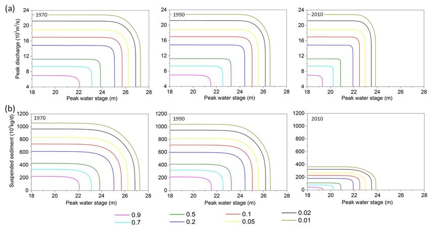
Water 2019, 11, 746                                                                                2 of 17

model [7,8]. Yet, the designs of hydraulic structures (e.g., dam spillways, dikes, and river channels),
cross drainage structures (e.g., culverts and bridges) and urban drainage systems require not only
peak discharge (Q) value but also peak water stage (Z) and suspended sediment load (S). In fact,
the multivariate frequency analysis can provide more comprehensive understanding of the flood event
than simple univariate analysis [9–13].
      Human intervention in river basins (e.g., urbanization), the effect of climatic variability (e.g.,
Pacific Decadal Oscillation), and increased greenhouse gasses have been suggested to cause the changes
in the magnitude and frequency of extreme floods [14]. Therefore, statistical characteristics (e.g., mean
and variance) of univariate flood variables as well as their dependence structure could be time-varying
under changing environments (climate change and/or human activities) [15]. To better adapt such
background, it is essential to identify a reasonable distribution framework to dynamically capture
the evolution of statistical characteristics [16]. Under the time-varying moments model, distribution
parameters can be expressed as functions of some physical variables including atmospheric and land
cover indices [17–19]. Thus, it is a feasible way to describe the external effects in the construction
of dependence structures. Copulas [20] allow researchers to easily construct the distribution by
estimating marginal distributions and their dependence separately [21]. The method could provide a
more convenient statistical tool for more flexibility in modeling the marginal distributions and their
dependence [22]. In recent years, copula function has become a popular tool for multivariate flood
frequency analysis [23–29].
      In this study, we focus on Q, Z and S observed at Waizhou station in the Ganjiang River basin,
which has undergone extensive urban and suburban development over the past 50 years. The mean
elevation of the main channel dominated by sediment supply deficit or surplus at the bed can exert
a direct influence on water stage [30]. The section-cross elevation in the downstream of Ganjiang
River displays a change process over the past decades [31]. Forest cover rate is a valuable indicator
of forests in a country or region, controlling runoff processes and sediment generation [32]. Forest
coverage rate of the Ganjiang River basin has increased from 41% to 69% due to large-scale forest
planting of the basin. Given the aforementioned physical correlations, the main channel elevation
(MCE) and forest cover rate (FCR) are chosen as explanatory variables for modeling the time variations
of Q, Z, and S of the Ganjiang River. Using time-varying copula model with the covariates MCE and
FCR, the nonstationary bivariate joint distributions of different flood variables (i.e., Z-Q and Z-S) are
constructed to analyze the evolution of the bivariate relationships of both Z-Q and Z-S, including their
joint probabilities and conditional probabilities of Q and S given water stage.
      This paper is organized as follows. The study region and the available data used in this study
are described in the next section. Then, the methodologies including marginal distribution and
copula model with time-varying parameters are presented. Based on deriving the best fitted marginal
distributions and copulas, the results about the time-variation of joint and conditional probability for
both Z-Q and Z-S are calculated. Finally, the main conclusions of the case study are summarized.

2. Study Region and Data
     The Ganjiang River, which is the largest tributary of the Poyang Lake basin, is situated in Jiangxi
Province (in Southeastern China) with a drainage area of 83,500 km2 (Figure 1). This study area belongs
to hilly region with the main land use type of woodland [33]. The Ganjiang River basin is located in
the subtropical humid monsoon climate zone with distinct seasonal variations, where the annual mean
precipitation is about 1680 mm. The heaviest rainfall occurs in the main flood season from April and
June, and often lasts 15 to 20 days due to monsoon and typhoon rainstorms [34].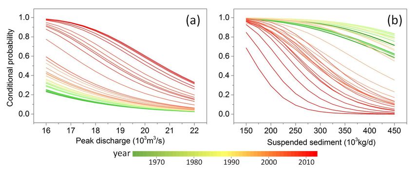
suspended sediment load (S) is calculated by multiplication between the daily discharge and the
corresponding suspended sediment rate. Then, the hydrological series of Q, Z and S are extracted
from the same flood event in each year with the maximum discharge value criterion. Besides, the
annual forest cover rates of the region are obtained from the book of China Compendium of Statis-
tics 1949–2008 [35] and Jiangxi provincial statistical yearbook from 1983 to 32014
Water 2019, 11, 746                                                                         of 17
(http://www.jxstj.gov.cn/).

       Figure 1.
       Figure    Topography and
              1. Topography and river
                                river channel
                                      channel of
                                              of the
                                                 the Ganjiang
                                                     Ganjiang River
                                                              River basin
                                                                    basin (GRB)
                                                                          (GRB) above
                                                                                above Waizhou
                                                                                      Waizhou station.
                                                                                               station.

      The catchment area upstream of the Waizhou station (115◦ 500 E, 28◦ 380 N) accounts for about
3. Methodology
97% of the total basin area of the Ganjiang River, and covers an area of 80,948 km2 (Figure 1).
      The time-varying
The hydrological      data copula
                            used inmodel,     in which
                                       this study         bothdaily
                                                    include     marginal
                                                                      river distributions
                                                                             discharge, dailyparameters     and copula
                                                                                                   water stage,   daily
suspended sediment rate and yearly section-cross elevation at the hydrological station fromthe
parameter     are  expressed   as  functions   of explanatory    variables,   is  constructed    to  describe      time
                                                                                                                1964  to
variations   of both  marginal   distribution   and  dependence     structure    of bivariate  flood
2013. These data are provided by the Hydrological Bureau of Jiangxi province (http://www.jxsw.cn/).    variables. Then,
joint
To    probability
    reflect          and conditional
            the capacity   of suspended probability
                                            sediment  that are derived
                                                        transport        from time-varying
                                                                    in a flood   event, suspended bivariate  copulaload
                                                                                                        sediment     are
illustrated
that  measuresto present  nonstationarity
                   the absolution   amountofofbivariate
                                                  sediment flood  variables
                                                              appears   to beover
                                                                                moretime.
                                                                                       reasonable than suspended
sediment rate, since the latter is a relative value for sediment. The daily suspended sediment load (S) is
3.1. Calculation of Explanatory Variables
calculated by multiplication between the daily discharge and the corresponding suspended sediment
rate. Change
      Then, theinhydrological
                    the main channel     of Q, Z and
                                  series elevation   ofSalluvial
                                                          are extracted
                                                                  rivers from    the same
                                                                          is a normal       flood
                                                                                         result     eventthe
                                                                                                 about     in hydraulic
                                                                                                              each year
with  the maximum
adjustments             discharge
                 to adapt           value criterion.
                           the variations              Besides,
                                             of discharge    andthe   annual forest
                                                                   sediment     load. cover
                                                                                       In thisrates   of the
                                                                                                 study,   theregion  are
                                                                                                              observed
obtained    from   the book  of  China   Compendium        of Statistics  1949–2008     [35]  and
cross-section elevation data for each year are tabulated and graphed as the profiles of the river   Jiangxi  provincial
statistical yearbook
cross-section.    Then,from   1983 to
                         the main      2014 (http://www.jxstj.gov.cn/).
                                     channel   elevations of 20 points are extracted from the cross-section

3. Methodology
     The time-varying copula model, in which both marginal distributions parameters and copula
parameter are expressed as functions of explanatory variables, is constructed to describe the time
variations of both marginal distribution and dependence structure of bivariate flood variables. Then,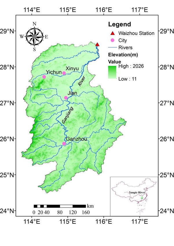
Water 2019, 11, 746                                                                                       4 of 17

joint probability and conditional probability that are derived from time-varying bivariate copula are
illustrated to present nonstationarity of bivariate flood variables over time.

3.1. Calculation of Explanatory Variables
     Change in the main channel elevation of alluvial rivers is a normal result about the hydraulic
adjustments to adapt the variations of discharge and sediment load. In this study, the observed
cross-section elevation data for each year are tabulated and graphed as the profiles of the river
cross-section. Then, the main channel elevations of 20 points are extracted from the cross-section
digitized graph from left to right bank [36]. To weaken the influence of some distortion/variability
points, the point elevations are divided into four quartiles and the 2nd quartile value is considered as
the main channel mean elevation (MCE) as follow:

                                              MCEt = Me(Ht )                                                 (1)

where Me(·) refers to the median of vector value Ht = (h1t , h2t , . . . , h20
                                                                            t
                                                                               ), which represents the bed
elevation value of the selected point.
      The forest landscape structure usually contains of the six forest cover classes (i.e., coniferous forest,
broadleaf forest, bamboo forest, mixed forest, economic forest, and shrubbery land). Each forest cover
with crown cover percent (cp) bigger than 20% has good effects on soil and water conservation [37].
Here, the criterion with this threshold value used in national forest definition is employed to calculate
forest area. Thus, the forest cover rate (FCR) is the percentage of six forest cover area to total land area
in a region and can be expressed as follow:

                                                6     Ait (cp > 0.2)
                                     FCRt =    ∑            AL
                                                                     × 100%                                  (2)
                                               i =1

where Ait (cp > 0.2) (i = 1,2, . . . , 6) is the six forest cover classes area with crown cover percent bigger
than 20%. AL stands for the total land area of the study region.

3.2. Marginal Distribution with Time-Varying Parameters
      To construct the dependence structure of bivariate hydrological variables by copulas, marginal
distribution of each variable should be determined firstly. In this study, five probability distributions,
including four two-parameter distributions (i.e., Lognormal, Weibull, Logistic, and Gamma) and
one three-parameter distributions (Pearson type III distribution) are selected as candidate marginal
distributions for Q, Z and S. These distributions have been widely applied in flood frequency
analysis [38,39]. The marginal distribution of a flood variable denoted by Y can be specified through a
parametric cumulative distribution function (CDF) FY (y|µ, σ, ν), where µ, σ and ν represent location,
scale and shape parameters, respectively, and are denoted by the vector θ = (µ, σ, ν) [40].
      The Generalized Additive Models for Location Scale and Shape (GAMLSS) introduced by Rigby
and Stasinopoulos [40] has been widely employed in nonstationary hydrological frequency analysis
for its flexibility [15,18,19,41]. If candidate marginal distribution function FY yt |θt is chosen to fit the


distribution of the variable yt at any time t, parameters of marginal distribution can be expressed as a
function of explanatory variables as follow:

                                      g(θ t ) = α0 + α1 MCEt + α2 FCAt                                       (3)

where g(·) represents the monotonic link function, which depends on the domain of statistical
parameter, i.e., if the domain of the distribution parameter θ t is θ t ∈ R, the link function is g θ t = θ t ,


or if θ t > 0, g θ t = ln θ t . θ t represents one of marginal distribution parameters (µt , σt , νt ). α0 , α1 ,


and α2 are the GAMLSS parameters. MCEt and FCAt represent two candidate explanatory variables.
In practice, the shape parameter νt (if it exists) is often treated as constant since it is quite unstable and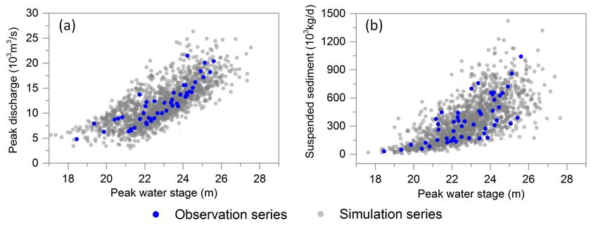
Water 2019, 11, 746                                                                                                 5 of 17

difficult to estimate [42], whereas time variations are considered only in location parameter µt and
scale parameter σt . What’s more, if the parameters are independent from the explanatory variables,
it would be a stationary distribution with constant parameters.
      The best fitted marginal distribution is determined by the Corrected Akaike Information Criterion
(AICc) [43], which is derived from the likelihood function with a penalty determined by the number
of model parameters. In addition, because of the potential drawbacks in the quality of the fitting of
AICc [44], the goodness-of-fit (GOF), which describes how well the selected distribution fits a set of
observations, for candidate distributions is assessed by the Kolmogorov–Smirnov (KS) test and Root
Mean Square Error (RMSE). Besides, visual assessment of the residual plot (QQ-plot) [45] is used to
examine the best fitted marginal distribution.

3.3. Time-Varying Bivariate Copula Model
     In practice, the implementation of the time-varying copula model could be divided into two
steps: fitting the time-varying marginal distribution of each variable firstly, and then estimating the
time-varying dependence structure of the copula. In other words, both the parameters of marginal
distribution and copula dependence parameter could be treated as time variation in building the
time-varying copula function. According to the definition of the copula [20], time-varying bivariate
copula function H (·) for the hydrological variable pairs of ( Z t , Qt ) and ( Z t , St ) at any time t can be
expressed as follows:
                               HZ,Q (zt , qt ) = C ( FZ (zt |θtz ), FQ (qt |θtq )|θzq
                                                                                    t )
                                                                                                             (4)
                               HZ,S (zt , st ) = C ( FZ (zt |θtz ), FS (st |θts )|θzs
                                                                                   t )

where C (·) represents bivariate copula function with time-varying dependence parameter θzq                          t or
  t
θzs . FZ (·), FQ (·) and FS (·) represent marginal cumulative distribution functions with corresponding
time-varying parameter vectors θtz = (µtz , σzt , νz ), θtq = (µtq , σqt , νq ), and θts = (µts , σst , νs ), respectively.
The joint distribution can be constructed by three Archimedean copula functions (i.e., Clayton,
Gumbel–Hougaard, and Frank, as shown in Table 1).

                         Table 1. The applied time-varying bivariate copulas in this study.

         Copula                 Cumulative Distribution Function with Time-Varying Parameters               Parameters
                                                                     t       t
                                                                                   −1/θ t
         Clayton                                 C (u, ν|θ t ) = (u)−θ + (ν)−θ − 1                            θt > 0

                                                                           t
                                                                                        t
                                                                                      t 1/θ
   Gumbel–Hougaard                        C (u, ν|θ t ) = exp − (− ln u)θ + (− ln ν)θ                         θt > 1
                         C (u, ν|θ t ) = − θ1t ln 1 + exp −uθ t − 1 × exp −νθ t − 1 / exp −θ t − 1            θ t 6= 0

          Frank

     Because of the impacts of external forces on the Ganjiang River basin, the dependence structure of
both Z-Q and Z-S could be nonstationary. Similar to the formula expression in Equation (3), the copula
dependence parameter could be expressed as a function of the two explanatory variables (FCR and
MCE) to reflect the nonstationarity of dependence structure. The totally four scenarios for copula
dependence parameter in this paper are listed as follows:

                                                      gc θct = β 0

                                                                                                                         (5)

                                                gc θct = β 0 + β 1 FCRt

                                                                                                                         (6)

                                               gc θct = β 0 + β 1 MCEt

                                                                                                                         (7)

                                         gc θct = β 0 + β 1 FCRt + β 2 MCEt

                                                                                                                         (8)

where gc (·) depends on the domain of copula dependence parameter θct , i.e., if θct ∈ R, the link function
is gc θct = θct or if θct > 0, gc θct = ln θct . β 0 , β 1 and β 2 are the model parameters.
Water 2019, 11, 746                                                                                         6 of 17

      The dependence parameter of Archimedean copula family can be estimated by Inference Function
for Margins method (IFM) [46]. The IFM method estimates the parameters through maximization of
the log-likelihood function of a copula. The most fitted copula function with time-varying dependence
parameter is determined by AICc criterion. The Cramér-von Mises test (CM) [47] and RMSE are used
to test the GOF of the copula functions. In addition, similar with the test of the univariate distribution,
QQ plot is also used to examine the best fitted copula based on the joint probability derived by the
selected copula.

3.4. Joint and Conditional Probability under Nonstationary Framework
     Joint probability gives the probability that each component falls in any particular range or discrete
set of values specified for these variables. Referring to the multivariate frequency analysis, the joint
probability of two variables usually includes three cases in general (i.e., KEN, OR, AND). Take AND
for the further analysis in this study, AND (∧) means the space in which all the variables exceed
corresponding values simultaneously [48]. Under the time-varying copula framework, the joint
              ∧ and P∧ can be calculated based on the best fitted copula function as follows:
probability PZQ        ZS

                       ∧ = P( Z ≥ z∗ ∧ Q ≥ q∗ )
                      PZQ

                           = 1 − FZ (z∗ |θtz ) − FQ (q∗ |θtq ) + C FZ (z∗ |θtz ), FQ (q∗ |θtq )|θzq
                                                                                                 t
                                                                                                               (9)
                       ∧ = P( Z ≥ z∗ ∧ S ≥ s∗ )
                      PZS
                          = 1 − FZ (z∗ |θtz ) − FS (s∗ |θts ) + C FZ (z∗ |θtz ), FS (s∗ |θts )|θzs
                                                                                                t


where z∗ , q∗ , and s∗ are the threshold values of Z, Q and S, respectively. In fact, a given joint probability
can correspond infinite data couples, among which there exist the most likely combination with the
largest probability density [49]. The most likely combinations conditioned on the given joint probability
k can be expressed as follows:

                       (z, q) = argmaxc FZ (z|θtz ), FQ (q|θtq )|θ ZQ
                                                                    t     · f Z z|θtz · f Q q|θtq
                                 H (z,q)=k
                                                                                                             (10)
                         (z, s) = argmaxc FZ (z|θtz ), FS (s|θts )|θ ZS
                                                                     t    · f Z z|θtz · f S s|θts

                                   H (z,s)=k

where c(·) represents copula density function. f Z (·), f Q (·) and f S (·) represent the marginal distribution
density functions of Z, Q and S, respectively. argmax stands for argument of the maxima, which is the
                                                              H (·)=k
set of points, (z, q) or (z, s), for which the function c(·) attains the function’s largest value conditioned
on H (·) = k.
      To display the time variation of flood variables with given water stage, the conditional probability
of peak discharge or suspended sediment load could be derived from the joint probability as Equation
(9). The conditional probability based on nonstationary bivariate copula can be expressed as follows:

                                                                               P( Z ≥z∗ ,Q≥q∗ )
                               P Q| Z = P ( Q ≥ q∗ | Z ≥ z∗ ) = 1 −                 P( Z ≥z∗ )

                                   1− FZ (z∗ |θtz )− FQ (q∗ |θtq )−C FZ (z∗ |θtz ),FQ (q∗ |θtq )|θ ZQ
                                                                                                   t
                               =
                                                              1− FZ (z∗ |θtz )
                                                                                         ∗       ∗           (11)
                               PS| Z = P(S ≥         s∗ | Z  ≥ z∗ ) = 1 − P(ZP≥(Zz≥,Sz∗≥)s )
                                   1− FZ (z∗ |θtz )− FS (s∗ |θts )−C ( FZ (z∗ |θtz ),FS (s∗ |θts )|θ ZS
                                                                                                     t
                                                                                                        )
                               =
                                                              1− FZ (z∗ |θtz )

4. Results
     The temporal trends of peak discharge, peak water stage and suspended sediment load are
investigated for selection of explanatory variables. Then, the marginal distributions of three flood
variables are described by time-varying distributions, and time-varying copulas are applied to construct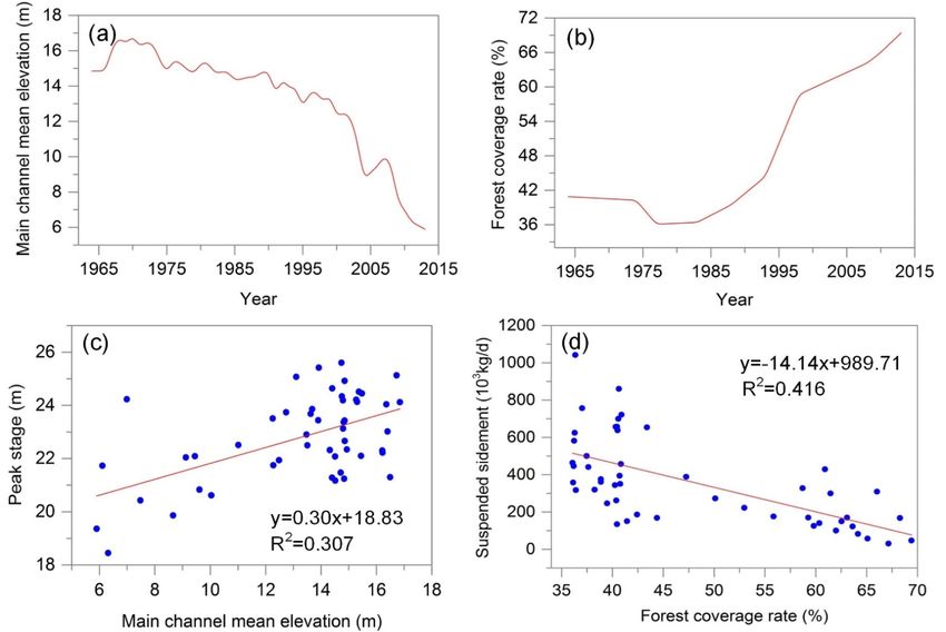
Water 2019, 11, 746 7 of 17
joint distributions of both Z-Q and Z-S. Finally, joint probability and conditional probability of bivariate
flood variables are estimated to display time variation of their joint distributions over time. The details
of the results are provided in the following sub-sections.
4.1. Temporal Trend Analysis
The nonstationarities of the flood series Q, Z and S at Waizhou station are examined by three
trend analysis methods, including the MK test, Spearman test and Kendall test. Results of the trend
analysis for Q, Z, and S are shown in Table 2. It is seen that the series of Z and S have undergone
significant decreasing trends at the 1% significance level during 1964–2013. Peak discharge Q has
presented some degree of negative trends, but cannot pass the trend tests at the 5% significance level.
The change of forest cover does not have strong effects on flood peak discharge during large storm
events, especially for large basins [50].
Table 2. Trend analysis of the three flood peak series at the Waizhou station during 1964–2013.
Annual Mean
Series MK Spearman Kendall
1964–2003 2004–2013
Q 12.01 10.47 −1.33 −0.16 −0.12
Z 23.25 20.96 −2.92 ** −0.41 ** −0.29 **
S 418.23 123.90 −5.33 ** −0.70 ** −0.52 **
Note: Q: peak discharge (103 m3 /s); Z: peak water stage (m); S: suspended sediment load (103 kg/d). –: delineates
negative trends; * and ** delineate significant trend at 0.05, 0.01 significance level, respectively.
The suspended sediment load has undergone significant decreasing trend, particularly after 2003
because of projects implementation about afforestation and conservation measures [51]. The river
elevation has undergone significant decrease due to river sand mining [31], which has intensified
obviously since 2003. In order to display the sharp changes of Q, Z, and S in the period of last decades,
the year of 2003 is chosen as a separated point from the inherent physical cause-effect connection.
The annual mean values of Z and S are about 23.25 m and 418.22 × 10³ kg/day from 1964 to 2003, and
then decrease to 20.96 m and 123.90 × 10³ kg/day for the last decade. Through the aforementioned
analysis, it is reasonable to conclude that both Z and S display significant nonstationarity during the
period from 1964 to 2013, whereas Q is stationary. The trend identification of Q, Z and S are consistent
with some previous research conclusions [52,53].
4.2. Nonstationary Marginal Distributions
According to the cause-effect analysis, MCE and FCR could be two potential physical driving
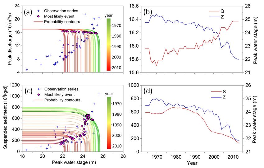
forces for the nonstationarity of Z and S. MCE series (Figure 2a) at Waizhou station have presented an
obvious decreasing trend from 1964 to 2013, especially during last ten years. FCR series (Figure 2b) of
Ganjiang River basin displays a slight decreasing trend before 1980s, but it expands rapidly from 1980s
to 2010s due to artificial afforestation and forest conservation in Jiangxi province. Figure 2c,d illustrate
significant positive correlation between Z and MCE, and significant negative correlation between S
and FCR, respectively. Considering their inherent physical connection as well as statistical correlation,
MCE and FCR are separately used as explanatory variables of the nonstationarity of Z and S.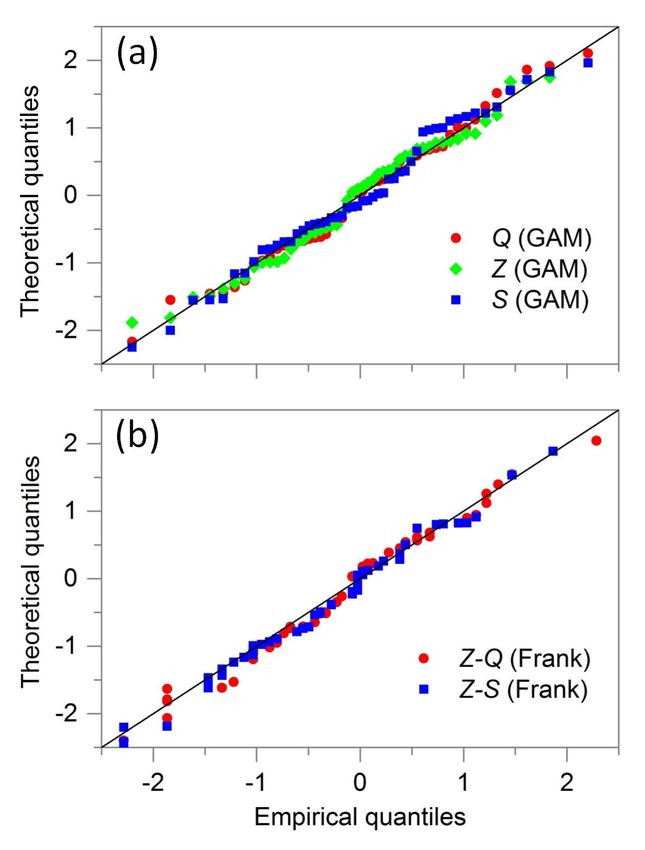
2b) of Ganjiang River basin displays a slight decreasing trend before 1980s, but it expands rapidly
from 1980s to 2010s due to artificial afforestation and forest conservation in Jiangxi province. Figure
2c,d illustrate significant positive correlation between Z and MCE, and significant negative correla-
tion between S and FCR, respectively. Considering their inherent physical connection as well as
statistical
Water correlation,
2019, 11, 746 MCE and FCR are separately used as explanatory variables of the nonstation-
8 of 17
arity of Z and S.
Figure 2.2. Data analyses of four variable series in the Ganjiang River basin (GRB) during 1964–2013. 1964–2013.
(a) is
is evolution
evolution of the
the main
main channel
channel mean elevation (MCE) at Waizhou station, (b) is evolution of
forest coverage
coveragerate
rate(FCR)
(FCR)ofofthe
theGRB,
GRB,and two
and twocorrelation
correlationplots areare
plots between peak
between water
peak stagestage
water (Z) and
(Z)
MCE
and MCE(c) and suspended
(c) and sediment
suspended load
sediment (S) (S)
load FCR
andand FCR(d),(d),
respectively. R2Rvalue
respectively. 2 valueisisthe
thesquare
square of
of the
correlation coefficient.
coefficient.
Since
Since annual
annual peak peakdischarge
dischargedisplays
displaysstationarity
stationarityduring
during 1964–2013,
1964–2013, Q is
Q fitted
is fittedby five candidate
by five candi-
distributions
date distributions withwithall parameters
all parameterstreated as constants.
treated as constants. InIn fittingZZand
fitting andSSseries
series by by nonstationary
nonstationary
models,
models, there
there are are three
three main
main possible
possible situations
situations for
for each
each candidate
candidate distribution:
distribution: (1)(1) only
only the
the location
location
parameter
parameter is time-varying, (2) only the scale parameter is time-varying and (3) both the location and
is time-varying, (2) only the scale parameter is time-varying and (3) both the location and
scale
scale parameters
parametersare aretime-varying.
time-varying.The The final distribution
final distribution modelmodel for each candidate
for each is determined
candidate is determinedfrom
the
from three models
the three aboveabove
models by the byselection criterion
the selection of AICc
criterion (i.e., (i.e.,
of AICc model withwith
model the minimum
the minimum AICc is the
AICc is
best). For the three flood variables Q, Z and S,
the best). For the three flood variables Q, Z and S, the estimated parameters and the results ofGOF
the estimated parameters and the results of the the
test
GOFoftestall candidate
of all candidatemarginal distributions
marginal are summarized
distributions are summarizedin Tablein3.Table
The P-value of the KSoftest
3. The P-value thewasKS
simulated using the Monte Carlo method. All the distributions pass the KS
test was simulated using the Monte Carlo method. All the distributions pass the KS test at the 0.01 test at the 0.01 significance
level. According
significance level. to AICc, thetomost
According AICc,appropriate marginal distributions
the most appropriate of Q, Z and
marginal distributions S are
of Q, Z andGammaS are
Gamma distribution. The location parameter μ of the Gamma distribution for describing Z is pos-
distribution. The location parameter µ of the Gamma distribution for describing Z is positively related
to MCE,related
itively whereas to the
MCE,scale parameter
whereas σ is constant.
the scale parameter σ is constant.
Meanwhile, both location and scale
Meanwhile, bothparameters
location and of
the
scaleGamma distribution
parameters for describing
of the Gamma S are positively
distribution related
for describing to FCR.
S are The QQ
positively plot (Figure
related to FCR.3a) The of QQ
the
best fitted distribution indicates that these selected distributions have a quite good
plot (Figure 3a) of the best fitted distribution indicates that these selected distributions have a quite fitting quality.
good fitting quality.Water 2019, 11, 746 9 of 17
Table 3. Parameters and goodness-of-fit of the candidate marginal distributions fitted to Q, Z, and S at
the Waizhou station during 1964–2013, respectively.
KS-Test
Variable Distribution Estimated Parameters AICc
Statistic p-Value
LNO m = 9.309, σ = 0.346 970.57 0.083 0.881
WEI µ = 13090, σ = 3.154 973.81 0.101 0.683
Q LOG µ = 11451, σ = 2305 976.57 0.108 0.602
GAM µ = 11703, σ = 0.339 970.48 0.097 0.737
PIII µ = 11694, σ = 0.350, γ = 0.474 971.89 0.080 0.910
LNO µ = exp (1.081 + 0.004MCEt ) 177.31 0.084 0.843
σ = 0.059
WEI µ = exp (3.005 + 0.011MCEt ) 181.46 0.101 0.646
σ = exp (2.123 + 0.061MCEt )
LOG µ = 18.461 + 0.326MCEt 179.09 0.081 0.873
Z
σ = 0.782
GAM µ = exp (2.946 + 0.014MCEt ) 177.24 0.089 0.793
σ = 0.059
PIII µ = exp(2.936+0.014MCEt ) 178.67 0.093 0.745
Σ = 0.060, γ = 0.251
LNO µ = exp (2.150 − 0.886FCRt ) 646.40 0.097 0.701
σ = exp (-1.332 + 1.378FCRt )
WEI µ = exp (8.072 − 4.544FCRt ) 648.35 0.136 0.285
σ = exp (1.476 − 1.448FCRt )
LOG µ=950.510 − 12.693FCRt 657.23 0.131 0.332
S
σ = exp (6.137 − 3.412FCRt )
GAM µ = exp (7.943 − 4.530FCRt ) 645.95 0.113 0.515
σ = exp (−1.336 + 1.291FCRt )
PIII µ = exp (8.098 − 4.854FCRt ) 646.05 0.084 0.845
σ = 0.537, γ = 0.702
Note: LNO, WEI, LOG, GAM and PIII are the abbreviations of Lognormal, Weibull, Logistic, Gamma and Pearson
type III distribution, respectively. MCE and FCR stand for the main channel mean elevation (m) and forest coverage
rate (%), respectively. µ, σ and ν represent location, scale and shape parameters of marginal distribution, respectively.
The best appropriate distribution marked with bold fonts.
Due to the balance of riverbed erosion and deposition during 1964–1994, the mean value of Z at
Waizhou station is about 23.26 m. In the period of 1995–2013, the value of MCE has underwent a sharp
decrease from 12.74 to 5.90 m, thus the variable value for Z has dropped obviously as well. Similarly,
the mean and coefficient of variation (Cv) of the suspended sediment load at Waizhou station are
469.81 × 10³ kg/day and 0.47 during 1964–1994. After 1995, the mean and Cv of S are getting smaller
significantly, because massive afforestation activities have been implemented in the study basin with
growth rate of forest cover at 1.17% year by year.
4.3. Nonstationary Dependence of Bivariate Flood Variables
Bivariate copulas under stationary and nonstationary conditions are constructed based on the
estimated marginal distributions. In modelling time-varying copula, selection of the explanatory
variables (i.e., MCE and FCR) is determined by the two corresponding marginal variables. In detail,
about the link function of copula parameter, MCE is selected as covariate expressed in Equation (6) for
Z-Q, while MCE and/or FCR are chosen as covariates described in Equations (7) and (8) for Z-S.
The results of the estimated parameters and GOF are summarized in Table 4. The P-value of the
CM test is simulated using the Monte Carlo method. All the applied copula functions pass the CM test
at the significance level of 0.01. Then, RMSE and AICc, which claim that the model with smaller values
is the better, are used as selected criteria [54]. Performances of the candidate copulas are not different
obviously from RMSE because of a little difference between them. But the optimum time-varying
copulas perform better than stationary ones for Z-Q and Z-S in terms of AICc. Frank is found to beWater 2019, 11, 746 10 of 17
t , θ t expressed in
the more appropriate bivariate copula for both Z-Q and Z-S, and parameters θ ZQ ZS
Equations (12) and (13), respectively, as below:
t
θ ZQ = 41.713 − 1.747MCEt (12)
t
θ ZS = 16.169 − 0.782MCEt (13)
Table 4. Parameters and goodness-of-fit of the candidate bivariate copulas fitted to Z-Q and Z-S at the
Waizhou station during 1964–2013, respectively.
CM-Test
Copula Parameter (θ) AICc RMSE
Statistic p-Value
5.702 −103.91 0.031 0.053 0.457
Clayton
exp (1.811 − 0.005MCEt ) −101.93 0.031 0.053 0.458
4.008 −94.76 0.039 0.056 0.426
Z-Q GH
exp (1.743 − 0.026MCEt ) −93.33 0.039 0.055 0.433
17.683 −102.79 0.035 0.055 0.434
Frank
41.713 − 1.747MCEt −104.25 0.035 0.054 0.448
1.250 −22.70 0.040 0.048 0.538
exp (−1.760 + 0.063FCRt ) −25.11 0.039 0.038 0.716
Clayton
exp (1.739 − 0.114MCEt ) −24.01 0.040 0.044 0.596
exp (−5.025 + 0.118FCRt − 0.113MCEt ) −23.48 0.040 0.052 0.479
1.796 −28.04 0.038 0.050 0.506
exp (0.350 + 0.007FCRt ) −26.25 0.039 0.047 0.541
Z-S GH
exp (1.195 − 0.045MCEt ) −27.40 0.038 0.047 0.556
exp (3.563 − 0.039FCRt − 0.128MCEt ) −26.76 0.039 0.057 0.410
5.319 −28.77 0.032 0.035 0.759
−1.528 + 0.226FCRt −28.79 0.032 0.029 0.855
Frank
16.169 − 0.782MCEt −30.29 0.031 0.028 0.870
24.186 − 0.132FCRt − 1.072MCEt −28.45 0.032 0.030 0.840
Figure 3b shows the QQ plot of the two bivariate copulas above. It displays a good agreement
between empirical distribution and theoretical distribution. In addition, graphical GOF of the selected
Frank copulas for both Z-Q and Z-S are shown in Figure 4. The simulation series of Q, Z, and S, which
are 30 scatters per year from 1964 to 2013, are generated by Monte Carlo method. Data are transformed
to the real space by use of the corresponding marginal distributions. This graphical GOF also
demonstrates that the selected time-varying copula functions have satisfactory fitting performances.Water 2019,11,
Water2019, 11,746 11 of
of 17
Water 2019, 11, xx FOR
FOR PEER
PEER REVIEW
REVIEW 11
11 of 17
17
Figure
Figure 3.Quantiles–Quantiles
Figure3.3. Quantiles–Quantiles
(QQ)
Quantiles–Quantiles plotplot
(QQ)
(QQ)
of the
of selected
plot of
marginal
the selected
the selected distributions
marginal
marginal
(a) and(a)
distributions
distributions
bivariate copula
and bivariate
(a) and bivariate
(b).
copula (b).
copula (b).
Figure
Figure 4.Scatter
Figure4.
4. Scatterplots
Scatter plotsof
plots ofZ-Q
of Z-Q(a)
Z-Q (a) andZ-S
(a)and
and Z-S(b)
Z-S (b)shown
(b) showncomparison
shown comparisonof
comparison ofobserved
of observed data
observed datawith
data withsets
with setsof
sets of1500
of 1500
1500
generated random
generated random samples
random samples based
samples based
based onon the
on the selected
the selected bivariate
selected bivariate copulas.
bivariate copulas. Solid
copulas. Solid circles
Solid circles in
circles in blue
in blue color
color are
blue color are
generated are
observed data
observed data and
data and gray
and gray dots
gray dots are
dots are simulated
are simulated samples.
simulated samples.
samples.
observed
Therefore, evolutions of the correlation parameters (i.e., θ ZQ t , θ t ) present the overall upward
(i.e., θ tt , θ tt )present the overall upward
ZS
Therefore,
trendTherefore,
evolutions
evolutions
significantly from 1964
of the
of the correlation
correlation
to 2013,
parameters
which parameters
can demonstrate θZQ
(i.e.,that , θZS
ZQthe ZS )present the
dependence overall upward
structures of Z-Q
trend
trend
and significantly
significantly
Z-S from 1964
from
are nonstationary. 1964 to 2013,
to
These 2013, which
which
results can demonstrate
can demonstrate
demonstrate that the
that
that riverbed thedown-cutting
dependence structures
dependence structures
instead ofofof Z-Q
Z-Q
forest
and Z-S
coverage are
is nonstationary.
the main externalThese
effect results
for both demonstrate
and that
at riverbed
Waizhou down-cutting
and Z-S are nonstationary. These results demonstrate that riverbed down-cutting instead of forest
Z-Q Z-S station. It is instead
possible to of forest
analyze
coverage
coverage
the is the
is the main
multivariate main
flood external
external effect
effect
frequency for
infor both
theboth Z-Qthrough
Z-Q
future and Z-S
and Z-Sthe
at Waizhou
at Waizhou
prediction station.
station. It is
It is possible
possible
of explanatory to analyze
to analyze
variables at
the multivariate
the multivariate flood
flood frequency
frequency in in the
the future
future through
through the
the prediction
prediction of of explanatory
explanatory variables
variables atatWater 2019, 11, 746 12 of 17
Water 2019, 11, x FOR PEER REVIEW 12 of 17
Waizhou stationbased
Waizhou station basedonontheir
their relationships
relationships [55,56].
[55,56]. Furthermore,
Furthermore, it give
it can can supporting
give supporting infor-
information
mation for the flood control design of hydraulic structures under the changing environments
for the flood control design of hydraulic structures under the changing environments [14,39]. [14,39].
4.4.
4.4. Temporal
Temporal Variation in Joint and Conditional Probabilities
Contours
Contours forfor various
various joint
joint probabilities
probabilities denoted
denoted in in Figure
Figure 55 are
are calculated
calculated by by using
using the
the selected
selected
copulas
copulas with
with parameters
parameters in in the
the years
years of
of 1970,
1970, 1990
1990 and
and 2010.
2010. With
With the
the same
same probability,
probability, Z maintains
maintains
generally higher and
generally higher andalmost
almostequivalent
equivalentvalue
value before
before 1990,
1990, whereas
whereas moves
moves downward
downward greatly
greatly fromfrom
1990
1990
to 2010to 2010
due toduethetodecrease
the decrease in mean
in mean of theofpeak
the peak
waterwater
stage.stage. Similarly,
Similarly, the value
the value of Srapidly
of S falls falls rap-
in
idly in last ten years due to the significant decrease in mean and Cv of S after 1995.
last ten years due to the significant decrease in mean and Cv of S after 1995. For example, the contoursFor example, the
contours
for 0.2 in for 0.2for
2010 in both
2010 Z
forand
both Z and
S are S are
lower lower
than than
lines for lines
0.7 infor 0.7and
1970 in 1970
1990,and 1990,indicates
which which indicates
that the
that the nonstationarity
nonstationarity playinfluence
play a great a great influence on joint probability
on joint probability in the last in the last
decade. decade.
Upon Upon
closer closer
inspection,
inspection, due to the strengthening in dependence for both Z-Q and Z-S, the
due to the strengthening in dependence for both Z-Q and Z-S, the corner of contour with the same corner of contour with
the
jointsame joint probability
probability becomesespecially
becomes angular, angular, especially for the
for the lower lower probability.
probability.
Figure 5.
Figure Jointprobability
5. Joint probabilitycontours
contourswith
withthe
thegiven P∧∧ (AND)
given P of Z-Q
(AND) of Z-Q (a) and Z-S
(a) and (b) using
Z-S (b) using the
the best
best
fitted bivariate copulas at the Waizhou station in the years of 1970, 1990 and 2010.
fitted bivariate copulas at the Waizhou station in the years of 1970, 1990 and 2010.
As shown in Figure 6, the temporal variations of joint probability as Equation (9) are assessed
As shown in Figure 6, the temporal variations of joint probability as Equation (9) are assessed
for each time step from 1964 to 2013. Meanwhile, the magenta dots on the probability contours
for each time step from 1964 to 2013. Meanwhile, the magenta dots on the probability contours rep-
represent the corresponding the most likely combination derived from Equation (10). The probability
resent the corresponding the most likely combination derived from Equation (10). The probability
contours cover a broad range, with marginal values ranging from 22.12 m to 25.06 m for Z and
contours cover a broad range, with marginal values ranging from 22.12 m to 25.06 m for Z and 721.78
721.78 × 10³ kg/day to 151.58 × 10³ kg/day for S. It can be seen that the suspended sediment load is
× 103 kg/day to 151.58 × 10³ kg/day for S. It can be seen that the suspended sediment load is more
more sensitive to flood event than the peak water stage from comparison of their value ranges. For the
sensitive to flood event than the peak water stage from comparison of their value ranges. For the
most likely combination, the peak discharge at Waizhou station in the Ganjiang River displays a slight
most likely combination, the peak discharge at Waizhou station in the Ganjiang River displays a
increasing trend from 15.97 × 10³ m3 /s3to 16.41 × 10³ m3 /s over time, while the values of peak water
slight increasing trend from 15.97 × 10 m /s to 16.41 × 10 m3/s over time, while the values of peak
3 3
stage and suspended sediment load have obviously decreased, especially in the last decade. As shown
water stage and suspended sediment load have obviously decreased, especially in the last decade.
in Figure 6b,d, it is indicated that Z and S in the most likely combination are obviously affected by
As shown in Figure 6b,d, it is indicated that Z and S in the most likely combination are obviously
riverbed down-cutting and the change of forest cover, respectively. Moreover, since the dependence
affected by riverbed down-cutting and the change of forest cover, respectively. Moreover, since the
structure of Z-Q is nonstationary as Equation (12), Q in the most likely combination is impacted by
dependence structure of Z-Q is nonstationary as Equation (12), Q in the most likely combination is
riverbed down-cutting as well.
impacted by riverbed down-cutting as well.Water 2019, 11, x FOR PEER REVIEW 13 of 17
Water 2019, 11, 746 13 of 17
Water 2019, 11, x FOR PEER REVIEW 13 of 17
Figure 6. Time variation of joint probability contours P∧ =0.1 for Z-Q (a) and Z-S (c) and corre-
sponding
Figure the most
6. Time likely
variation ofcombinations forcontours
joint probability Z-Q (b) P
and
∧ =Z-S∧ (d)
0.1 for derived from
Z-Q (a) and the
Z-S (c)best
and fitted bivariate
corresponding
Figure 6. Time variation of joint probability contours P =0.1 for Z-Q (a) and Z-S (c) and corre-
copula
the mostatlikely
the Waizhou station
combinations forfrom
Z-Q 1964 to 2013.
(b) and Z-S (d) derived from the best fitted bivariate copula at the
sponding the most likely combinations
Waizhou station from 1964 to 2013. for Z-Q (b) and Z-S (d) derived from the best fitted bivariate
copula
The at the Waizhou
conditional station from
probability 1964 to 2013.
as Equation (11) is calculated by the best fitted copula function for
both TheZ-Qconditional
and Z-S. In probability
practice, flood as Equation (11) is calculated
control planners and managers by the best fitted
usually focuscopula
on thefunction
water stage for
both The
ratherZ-Q thanconditional
anddischarge probability
Z-S. In practice, as Equation
flood control
and suspended (11)
planners
sediment is calculated
load and managers
in severe by the best
floodusually fitted copula
focus the
flow. Given on the function
water water
warning stagefor
both Z-Q thanand Z-S. In practice, flood control planners and managers
flood usually focustheon warning
the
Q|Z water S|Z stage
rather
stage (23.5 discharge
m) at Waizhouand suspended
station, thesediment load in
time variations severe
of conditional flow. Given
probability ( P , P )water from
stage (23.5 m) at Waizhou station, the time variations of conditional probability (P , P ) fromwater
rather than discharge and suspended sediment load in severe flood flow. Given Q the
| Z warning
S | Z 1964
1964 to 2013 are presented in Figure 7. The result can be of great important and noteworthy Q|Z S|Z for
to 2013(23.5
stage are presented
m) at Waizhou in Figure 7. The
station, theresult
time can be of great
variations important probability
of Qconditional
|Z
and noteworthy ( P ,
forP spillway
) from
spillway
design design and flood control. It can be | Z forthat
PQseen P discharge
for the fixed discharge hastime,increased
1964 toand flood
2013 arecontrol.
presented It caninbe seen
Figure that
7. The resultthe
canfixed has increased
be of great important andover noteworthy while for
P S | Z S | Z
has decreasedPduring last fifty years. That’s to say, evenQif|Z Z maintains the same value at Waizhou
over time,design
spillway while and flood has control.
decreased during
It can last fifty
be seen P That’s
that years. for thetofixed
say, discharge
even if Z maintains
station, the fact should attract more attention that probabilities of inundation and riverbed erosion are
has increased the
same value at Waizhou S |Z station, the fact should attract more attention that probabilities of inundation
getting
over time,higher fromP1964
while to 2013.
has decreased during last fifty years. That’s to say, even if Z maintains the
and riverbed erosion are getting higher from 1964 to 2013.
same value at Waizhou station, the fact should attract more attention that probabilities of inundation
and riverbed erosion are getting higher from 1964 to 2013.
Figure 7. Time variation of conditional probability P Q| Z Q(a)
|Z and P
S| Z (b) with the given warning water
S |Z
Figure 7. Time variation of conditional probability P (a) and P (b) with the given warning
stage (Z ≥ 23.5 m) at the Waizhou station from 1964 to 2013.
water stage (Z ≥ 23.5 m) at the Waizhou station from 1964 to 2013.
Q|Z S |Z
Figure 7. Time variation of conditional probability P (a) and P (b) with the given warning
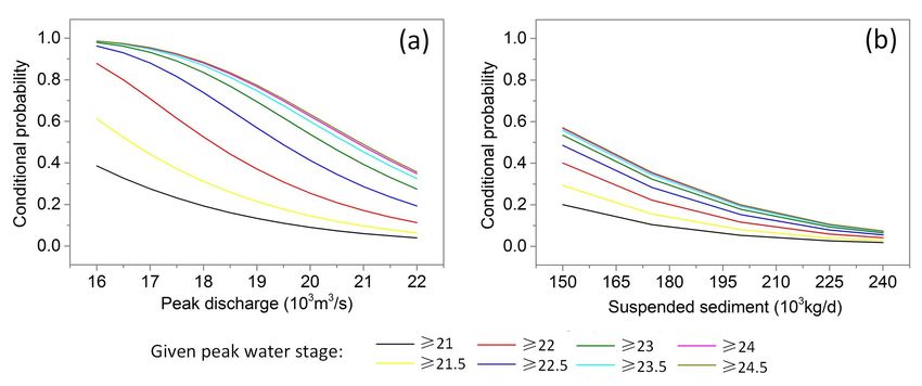
What is more, the proposed method also allows us to obtain more information concerning the
water stage
What (Z ≥the
is more, 23.5proposed
m) at the Waizhou
methodstation from 1964
also allows us to to obtain
2013. more information concerning the
conditional probabilities under various given water stages. Figure 8 has shown the results, where MCE
conditional probabilities under various given water stages. Figure 8 has shown the results, where
and FCR are assumed to be 6 m and 70%, respectively. The conditional probabilities become bigger for
MCE What is more,
and FCR the proposed
are assumed to be method
6 m andalso allows
70%, us to obtain
respectively. more information
The conditional concerning
probabilities the
become
both Q and S with the higher peak water stage. When values of Q and S become bigger, the differences
conditional probabilities under various given water stages. Figure 8 has shown the results,
bigger for both Q and S with the higher peak water stage. When values of Q and S become bigger, where
of conditional
MCE and FCRprobabilities
are assumedareto getting
be 6 m smaller under
and 70%, various given
respectively. water stages,
The conditional especially for
probabilities PS| Z
become
bigger for both Q and S with the higher peak water stage. When values of Q and S become bigger,Water 2019, 11, x FOR PEER REVIEW 14 of 17
the differences of conditional probabilities are getting smaller under various given water stages,
Water 2019, 11, 746 14 of 17
especially for P S |Z (Figure 8b). In addition, the conditional probability PQ|Z is more sensitive
S |Z
than P on condition of various water stages at Waizhou station. Those results can give us
(Figure 8b). In addition, the conditional probability PQ| Z is more sensitive than PS| Z on condition of
quantitative
various waterinformation about temporal
stages at Waizhou station. variation of flood
Those results variables
can give under the information
us quantitative changing environ-
about
ments in the Ganjiang River basin.
temporal variation of flood variables under the changing environments in the Ganjiang River basin.
Figure 8. Conditional probability P Q| ZQ|Z(a) and PS| Z (b)
S |Z with various given water stages when main
Figure 8. Conditional probability P (a) and P (b) with various given water stages when
channel elevation and forest coverage rate are assumed to be 6 m and 70%, respectively.
main channel elevation and forest coverage rate are assumed to be 6 m and 70%, respectively.
5. Conclusions
5. Conclusions
This study employs time-varying copula model to investigate the evolution of the relationships
of Z-Q and
This Z-S depending
study on main channel
employs time-varying copulaelevation
model to(MCE) and forest
investigate coverageofratio
the evolution (FCR) in the
the relationships
Ganjiang River basin during 1964–2013. The main conclusions are presented as follows:
of Z-Q and Z-S depending on main channel elevation (MCE) and forest coverage ratio (FCR) in the
Ganjiang River basin during 1964–2013. The main conclusions are presented as follows:
1. It is obvious that both the mean and variance of S have significantly decreased, while only the
1. Itmean
is obvious that both
has reduced for the mean and variance
Z, particularly of S have
in the recent significantly
decades. decreased,
Furthermore, Gamma while only the
distribution
mean has reduced for Z, particularly in the recent decades. Furthermore,
with location parameter expressed as a function of MCE is best fitted distribution for Z, and Gamma distribution
with
Gamma location parameter expressed
with parameters of locationasand a function of MCEasisfunctions
scale expressed best fittedofdistribution
FCA is for S,for Z, and
while the
Gamma with parameters of location and scale expressed
best fitted distribution of Q is the Gamma with constant parameters. as functions of FCA is for S, while the
2. best
It is fitted
found distribution
that the mostof Q fitted
is the Gamma
bivariatewith constant
copulas for parameters.
both Z-Q and Z-S are Frank copula,
2. Ittheis parameters
found that of the most fitted bivariate copulas for
which are expressed as the function of MCE. both Z-Q and Z-S riverbed
Therefore, are Frank copula, the
down-cutting
parameters of which are expressed as the function of MCE. Therefore, riverbed
at Waizhou station plays the dominant role in strengthening dependences of both Z-Q and Z-S down-cutting at
Waizhou
from 1964station
to 2013.plays the dominant role in strengthening dependences of both Z-Q and Z-S
3. from
The results of2013.
1964 to joint probability and conditional probability show that the corner of contour lines
3. The results of joint
enhanced more greatly probability
due to theandstrengthening
conditional probability
dependences show that
over the especially
time, corner of contour lines
for the lower
enhanced
probability.more greatly itdue
In addition, cantobe the
seenstrengthening
that values of dependences over time,
Z and S fall rapidly in theespecially
last ten yearsfor due
the
lower probability. In addition, it can
to the decreasing mean of these two variables. be seen that values of Z and S fall rapidly in the last ten
years due to the decreasing mean of these two variables.
Author Contributions: Data curation, T.W. and X.X.; Methodology, C.J. and T.W.; Software, T.W.; Formal
Author Contributions: Data curation, T.W. and X.X.; Methodology, C.J. and T.W.; Software, T.W.; Formal analysis,
analysis,
T.W.; T.W.;review
Writing, Writing,
andreview and
editing, editing,
T.W. T.W.
and C.J.; and C.J.;
Funding Funding C.J.
acquisition, acquisition, C.J.reviewed
All authors All authors
thereviewed the
manuscript.
manuscript.
Funding: This research is financially supported jointly by the National Natural Science Foundation of China
(NSFC Grant
Funding: This51809243),
research isWater Resources
financially Science
supported and Technology
jointly Project
by the National of Jiangxi,
Natural China
Science (201821ZDKT07,
Foundation of China
KT201704, KT201601, KT201508, KT201501), Science and Technology Project of Jiangxi, China
(NSFC Grant 51809243), Water Resources Science and Technology Project of Jiangxi, China (201821ZDKT07,(2015ZBBF60006),
the Fundamental Research Funds for the Central Universities (Grant CUG170679), Natural Science Foundation of
KT201704, KT201601, KT201508, KT201501), Science and Technology Project of Jiangxi, China (2015ZBBF60006),
Hubei Province (Project NO. 2018CFB270), all of which are greatly appreciated.
the Fundamental Research Funds for the Central Universities (Grant CUG170679), Natural Science Foundation
Conflicts of Interest:
of Hubei Province The authors
(Project declare no conflict
NO. 2018CFB270), of interest.
all of which are greatly appreciated.
Conflicts of Interest: The authors declare no conflict of interest.Water 2019, 11, 746 15 of 17
References
1. Zhong, Y.X.; Guo, S.L.; Liu, Z.J.; Wang, Y.; Yin, J.B. Quantifying differences between reservoir inflows and
dam site floods using frequency and risk analysis methods. Stoch. Environ. Res. Risk Assess. 2017, 32, 1–15.
[CrossRef]
2. Tena, A.; Batalla, R.J.; Vericat, D.; Lopez-Tarazon, J.A. Suspended sediment dynamics in a large regulated
river over a 10-year period (the lower Ebro, NE Iberian Peninsula). Geomorphology 2011, 125, 73–84. [CrossRef]
3. Ahn, J.; Cho, W.; Kim, T.; Shin, H.; Heo, J.-H. Flood frequency analysis for the annual peak flows simulated
by an event-based rainfall-runoff model in an urban drainage basin. Water 2014, 6, 3841–3863. [CrossRef]
4. Benkhaled, A.; Higgins, H.; Chebana, F.; Necir, A. Frequency analysis of annual maximum suspended
sediment concentrations in Abiodwadi, Biskra (Algeria). Hydrol. Process. 2014, 28, 3841–3854. [CrossRef]
5. Xu, W.T.; Jiang, C.; Yan, L.; Li, L.Q.; Liu, S.N. An adaptive metropolis-hastings optimization algorithm of
Bayesian estimation in non-stationary flood frequency analysis. Water Resour. Manag. 2018, 32, 1343–1366.
[CrossRef]
6. Blazkova, S.; Beven, K. Flood frequency prediction for data limited catchments in the Czech Republic using
a stochastic rainfall model and TOPMODEL. J. Hydrol. 1997, 195, 256–278. [CrossRef]
7. Iacobellis, V.; Fiorentino, M.; Gioia, A.; Manfreda, S. Best fit and selection of theoretical flood frequency
distributions based on different runoff generation mechanisms. Water 2010, 2, 239–256. [CrossRef]
8. Gioia, A.; Manfreda, S.; Iacobellis, V.; Fiorentino, M. Performance of a theoretical model for the description
of water balance and runoff dynamics in Southern Italy. J. Hydrol. Eng. 2014, 19, 1123–2014. [CrossRef]
9. Volpi, E.; Fiori, A. Design event selection in bivariate hydrological frequency analysis. Hydrol. Sci. J. 2012, 57,
1506–1515. [CrossRef]
10. Shafaei, M.; Fakheri-Fard, A.; Dinpashoh, Y.; Mirabbasi, R.; De Michele, C. Modeling flood event
characteristics using D-vine structures. Theor. Appl. Climatol. 2017, 130, 713–724. [CrossRef]
11. Salvadori, G.; Durante, F.; De Michele, C.; Bernardi, M. Hazard assessment under multivariate distributional
change-points: Guidelines and a flood case study. Water 2018, 10, 751. [CrossRef]
12. De Michele, C.; Salvadori, G.; Vezzoli, R.; Pecora, S. Multivariate assessment of droughts: Frequency analysis
and dynamic return period. Water Resour. Res. 2013, 49, 6985–6994. [CrossRef]
13. Vezzoli, R.; Salvadori, G.; Michele, C.D. A distributional multivariate approach for assessing performance of
climate-hydrology models. Sci. Rep. 2017, 7, 12071. [CrossRef]
14. Salas, J.D.; Obeysekera, J. Revisiting the concepts of return period and risk for nonstationary hydrologic
extreme events. J. Hydrol. Eng. 2014, 19, 554–568. [CrossRef]
15. Jiang, C.; Xiong, L.H.; Xu, C.-Y.; Guo, S.L. Bivariate frequency analysis of nonstationary low-flow series
based on the time-varying copula. Hydrol. Process. 2014, 29, 1521–1534. [CrossRef]
16. Gilroy, K.L.; Mccuen, R.H. Anonstationary flood frequency analysis method to adjust for future climate
change and urbanization. J. Hydrol. 2012, 414, 40–48. [CrossRef]
17. Steinschneider, S.; Brown, C. Influences of North Atlantic climate variability on low-flows in the Connecticut
River Basin. J. Hydrol. 2011, 409, 212–224. [CrossRef]
18. López, J.; Francés, F. Non-stationary flood frequency analysis in continental Spanish rivers using climate and
reservoir indices as external covariates. Hydrol. Earth Syst. Sci. 2013, 17, 3189–3203. [CrossRef]
19. Ahn, K.-H.; Palmer, R.N. Use of a nonstationary copula to predict future bivariate low flow frequency in the
Connecticut River basin. Hydrol. Process. 2016, 30, 3518–3532. [CrossRef]
20. Nelsen, R.B. An Introduction to Copulas; Springer: New York, NY, USA, 2006.
21. Kwon, H.H.; Lall, U. A copula-based nonstationary frequency analysis for the 2012–2015 drought in
California. Water Resour. Res. 2016, 52, 5662–5675. [CrossRef]
22. Grimaldi, S.; Serinaldi, F. Asymmetric copula in multivariate flood frequency analysis. Adv. Water Resour.
2006, 29, 1155–1167. [CrossRef]
23. Bezak, N.; Mikoš, M.; Šraj, M. Trivariate frequency analyses of peak discharge, hydrograph volume and
suspended sediment concentration data using copulas. Water Resour. Manag. 2014, 28, 2195–2212. [CrossRef]
24. Xing, Z.Q.; Yan, D.H.; Zhang, C.; Wang, G.; Zhang, D.D. Spatial Characterization and Bivariate Frequency
Analysis of Precipitation and Runoff in the Upper Huai River Basin, China. Water Resour. Manag. 2015, 29,
3291–3304. [CrossRef]You can also read