RF Loss Model for Tree Canopies with Varying Water Content
←
→
Page content transcription
If your browser does not render page correctly, please read the page content below
Journal of Electromagnetic Analysis and Applications, 2021, 13, 83-101
                                                                                                https://www.scirp.org/journal/jemaa
                                                                                                              ISSN Online: 1942-0749
                                                                                                                ISSN Print: 1942-0730

RF Loss Model for Tree Canopies with Varying
Water Content

Sonam Peden1,2*, Ronald C. Bradbury1, David William Lamb1,3, Mark Hedley4
1
 Precision Agriculture Research Group, University of New England, Armidale, NSW, Australia
2
 College of Science and Technology, Royal University of Bhutan, Rinchending, Bhutan
3
 Food Agility Cooperative Research Centre, University of New England, Armidale, NSW, Australia
4
 CSIRO Data61, Marsfield, NSW, Australia

How to cite this paper: Peden, S., Brad-        Abstract
bury, R.C., Lamb, D.W. and Hedley, M.
(2021) RF Loss Model for Tree Canopies          Detection of plant water status is important for monitoring plant physiology.
with Varying Water Content. Journal of          Previous studies showed that radio waves are attenuated when passing
Electromagnetic Analysis and Applications,
                                                through vegetation such as trees, and models (both empirical and analytical)
13, 83-101.
https://doi.org/10.4236/jemaa.2021.136006       were developed. However, for models to be more broadly applicable across a
                                                broad range of vegetation types and constructs, basic electrical properties of
Received: June 3, 2021                          the vegetation need to be characterised. In our previous work, a model was
Accepted: June 27, 2021
Published: June 30, 2021
                                                developed to calculate the RF loss through vegetation with varying water
                                                content. In this paper, the model was extended to calculate RF loss through
Copyright © 2021 by author(s) and               tree canopies with or without an air gap. When the model was compared with
Scientific Research Publishing Inc.
                                                the actual RF loss acquired using Eucalyptus blakelyi trees (with and without
This work is licensed under the Creative
Commons Attribution International               leaves), there was a systematic offset equivalent to a residual moisture content
License (CC BY 4.0).                            of 13% that was attributed to bound water. When the model was adjusted for
http://creativecommons.org/licenses/by/4.0/     the additional water content, the effective water path (EWP) was found to ex-
               Open Access
                                                plain 72% of the variance in the measured RF loss.

                                                Keywords
                                                Radio Attenuation, Water Content, Vegetation Thickness, Permittivity, Path
                                                Loss

                                              1. Introduction
                                              Eucalypts are iconic Australian forest trees. The Eucalyptus forest type is by far
                                              the most common forest type in Australia covering 101 million hectares, which
                                              is 77% of Australia’s total native forest area [1]. The prolonged drought experi-
                                              enced in southern Australia between 1996 and 2010 (the Millennium Drought)

DOI: 10.4236/jemaa.2021.136006         Jun. 30, 2021               83            Journal of Electromagnetic Analysis and Applications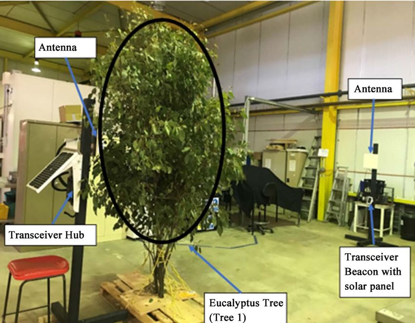
S. Peden et al.

                                 caused widespread mortality and secondary insect attack in both eucalypt native
                                 forests and pine plantations [2]. Species composition has also changed in re-
                                 sponse to prolonged lower rainfall [3]. Since the mid-1990s, mainland southeast
                                 Australia has experienced an 11 percent reduction in April-October rainfall.
                                 Drought makes vegetation more flammable, and therefore more likely to sup-
                                 port extreme bushfire behaviour [4].
                                   Water stress affects plant growth and development due to reduction in pho-
                                 tosynthetic activities [5] [6] [7] and hence affects forest productivity [8] [9].
                                 Canopy leaf wilting is considered an important visible symptom of drought,
                                 when water loss by transpiration is greater than absorption by the roots [10]
                                 [11]. The detection of plant water status is important for monitoring the
                                 physiological status of plants, and the assessment of drought and fire risk in
                                 natural plant communities, and the irrigation scheduling of crops [12] [13]. Al-
                                 though field sampling of single leaves and shoots provides the most accurate as-
                                 sessment of plant water status, such methods are not feasible when estimates are
                                 required for large areas of vegetation [14].
                                   Radio signals are attenuated when passing through vegetation due to absorp-
                                 tion and scattering by the discrete elements such as the branches, stems and
                                 leaves [15] [16] [17]. The so-called RF loss has been measured for specific fre-
                                 quencies in particular situations (forest, apple orchard & coconut garden for
                                 example) and empirical models have been developed from such measurements
                                 [16] [18] [19] [20] [21] [22]. Analytical models have also been developed but the
                                 more accurate Radiative Energy Transfer (RET) models depend on experimental
                                 measurements for their formulation and validation [23]. For a model to be ac-
                                 curate across a broad range of vegetation however, the relevant electrical char-
                                 acteristics of the vegetation need to be incorporated into the model.
                                   Radio waves interact strongly with water [24] and eucalyptus trees are no ex-
                                 ception. While RF loss measurements at any radio frequency would be related to
                                 water content, some frequency bands are more suitable than others. Below about
                                 600 MHz, the main RF loss mechanism involves the movement of ions. RF loss
                                 then is highly dependent on the medium’s electrical conductivity and hence the
                                 concentration of dissolved ions. Such information would be difficult to obtain
                                 for different species of vegetation which presents a hurdle for practical estima-
                                 tion of water content. Above about 1 GHz and up to 100 GHz, the main RF loss
                                 mechanism is the rotation of water molecules resulting from interaction between
                                 the radio signal electric field and the molecular electric dipole [25] [26]. Fre-
                                 quencies above 1 GHz have an advantage in that electrical conductivity does not
                                 play a significant part hence avoiding the need to characterize the highly-variable
                                 constituents of electric conductivity in leaves. The higher frequency also offers
                                 another advantage; namely directional antennas that can be used to facilitate lo-
                                 cation-specific measurements are smaller.
                                   Le Vine and Karam [27] calculated the attenuation associated with a vegeta-
                                 tion canopy using a discrete scatter model, where the vegetation canopy is pre-

DOI: 10.4236/jemaa.2021.136006                         84           Journal of Electromagnetic Analysis and Applications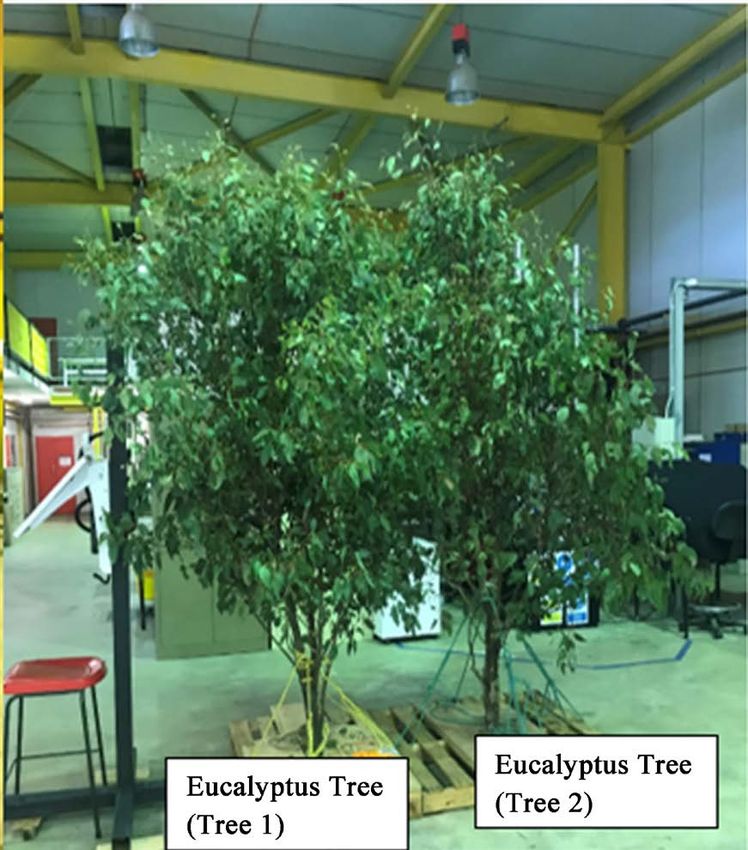
S. Peden et al.

                                 sented by a sparse layer of discrete, randomly oriented particles such as leaves,
                                 stalks, branches, etc over a homogeneous ground plane (soil). They found that
                                 for frequencies up to 5 GHz the attenuation varies approximately linearly with
                                 plant water content over the range 0.2 to 0.5 (by volume). Nakajima, et al. [28]
                                 measured the RF attenuation of individual leaves at 5, 10 and 20 GHz in a
                                 waveguide. They also investigated the effect in a living tree by measuring RF at-
                                 tenuation at 10.5 GHz. They asserted that “Microwave attenuation by tree foliage
                                 should have a strong link to water content in the leaves”. The dependency of at-
                                 tenuation on water content is through the dielectric constant which itself is
                                 highly dependent on the water content inside the material.
                                   The water inside vegetation (leaves and stems) can be divided into free water
                                 and bound water. Free water is the liquid water found in cell lumen and is rela-
                                 tively easy to remove [29]. Bound water is the water molecules that penetrate the
                                 cell walls and are chemically bound to cellulose molecules. Bound water cannot
                                 always be expelled by heat without damaging the material [30] and the removal
                                 of bound water also depends on the temperature and relative humidity of the
                                 environment [31].
                                   Previous studies showed that the RF loss through vegetation is strongly de-
                                 pendent on the water content in vegetation through its dielectric constant. Ulaby
                                 and El-Rayes [32] describe the relationship between water content and dielectric
                                 constant, detailed later in this paper. The relationship between RF loss and water
                                 content, however, has not been quantified.
                                   In our previous paper, we developed a model to calculate the RF loss through
                                 packed Eucalyptus leaves [33]. In this work, we extend our previous model to
                                 calculate the radio frequency (RF) signal loss through tree canopies (combina-
                                 tion of vegetation and air) and the model was compared against experimental
                                 measurements of RF loss for Eucalyptus tree canopies at 2.4 GHz. The key things
                                 are 1) to derive a model relating RF loss and water content; 2) using cut trees so
                                 that water content could be found by weighing; 3) air-drying to vary the water
                                 content while keeping the structure of the tree intact; 4) done inside to reduce
                                 environmental changes (rain, wind, temperature) that might otherwise affect
                                 measurements.

                                 2. Model
                                 In the following model derivation, the radio wave electric field is first related to
                                 the intrinsic impedance and complex propagation constant of each medium in
                                 the path. Those two parameters are then related to the corresponding complex
                                 permittivity of each medium. Permittivity, in turn, is related further to the vol-
                                 ume fractions of the substances (especially water) within the media.

                                 2.1. Wave Propagation
                                 We assume a plane wave travels through a set of slabs. In the case of a packed
                                 canopy (a group of trees with no space in between), each slab in the model

DOI: 10.4236/jemaa.2021.136006                        85            Journal of Electromagnetic Analysis and Applications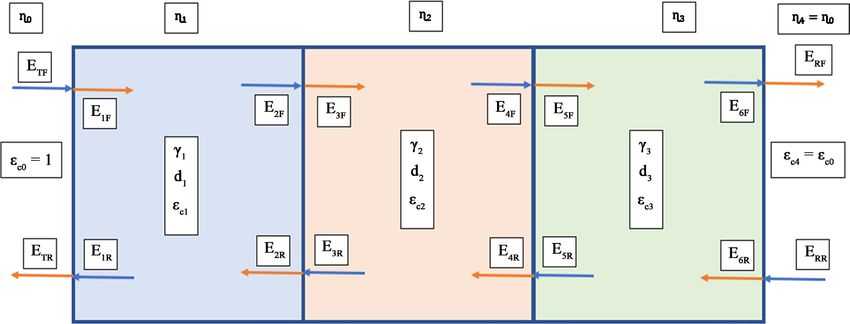
S. Peden et al.

                                         represents one tree. For an open canopy on the other hand, each tree and each
                                         space between the trees is represented by a slab in the model (refer Figure 1).
                                           Each tree is assumed to be a homogenous, lossy medium. Also, we assume
                                         that the material is non-magnetic.
                                           In Figure 2, we suppose that a radio wave is emitted from a transmitting an-
                                         tenna on the left, travels from left-to-right through the media and proceeds to a
                                         receiving antenna on the right. We are interested in the RF loss in intensity
                                         above the free-space loss. The model considers three components to the RF loss:
                                         1) partial transmission at the interfaces; 2) partial reflection at the interfaces and
                                         3) absorption by the lossy media.
                                           When an incident electromagnetic wave with electric field phasor, ETF is inci-
                                         dent at the first interface, it is partially transmitted and partially reflected. The
                                         transmitted wave, E1F propagates through first lossy medium with a complex

                                      Figure 1. Model when transmitted wave propagates through (a) N number of trees placed
                                      in series without an air gap in between the trees and (b) N number of trees placed in series
                                      with N-1 air gaps in between the trees.

        Figure 2. Structure of 3 lossy medium slabs and 4 interfaces. Symbols for the electromagnetic properties of the materials
        are defined. When a plane radio wave travelling left-to-right meets the medium it is partially transmitted and partially re-
        flected at the first interface. The transmitted wave propagates through the lossy medium with a complex propagation con-
        stant γ1. At the second interface it is again partially transmitted and partially reflected, the transmitted wave propagates
        through second medium and so on until it transmits back in to the air.

DOI: 10.4236/jemaa.2021.136006                                  86             Journal of Electromagnetic Analysis and Applications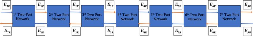
S. Peden et al.
propagation γ1, intrinsic impedance η1 and thickness d1 in metres. At the second
interface it is again partially transmitted and partially reflected, the transmitted
wave again passes through second lossy medium and so on until it transmits
through the last interface into the air as ERF. As a result of the reflections there is
a reverse-travelling wave also, denoted with subscript R.
In Figure 2, γ1, γ2, γ3 are the complex propagation constants in the 3 different
media with thicknesses d1, d2, d3, intrinsic impedances η1, η2, η3 and complex
permittivity εc1, εc2, εc3 respectively.
We consider Figure 2 to be cascaded two-port networks and the number of
two-port networks with their terminals according to Figure 2 are shown in Fig-
ure 3.
2.1.1. First Two-Port Network
The combined effect of cascaded two-port networks is found by multiplying the
individual T-parameter matrices, but S-parameters are more intuitive. The
S-parameter matrix equation is found first and then converted to a T-parameter
equation.
The first two-port network represents the interaction of the radio waves at the
left-most interface in Figure 2. The incoming phasors, ETF and E1R, are related to
the outgoing phasors, ETR and E1F, by an S-parameter matrix [34] as
ETR Γ 01 t10 ETF
E = t , (1)
1F 01 Γ10 E1R
where, t01 and t10 are the transmission coefficients of a forward and reverse trav-
elling waves through the first interface respectively, Γ10 and Γ01 are the re-
verse-to-forward and forward-to-reverse reflection coefficients when waves are
reflected from the first interface (air-to-first lossy medium interface). The
transmission coefficients, t01 and t10 are complex and these represent both the
amplitude change and the radio signal phase shift that occurs when the wave
passes through the interfaces. Likewise, the reflection coefficients, Γ10 and Γ01 are
complex and represent the amplitude and phase shift from reflection. These
terms are expressed in the following Equations (2)-(5) [35]:
η0 − η1 ε c1 − ε c 0
=
Γ10 = , (2)
η0 + η1 ε c1 + ε c 0
η − η0 ε − ε c0
Γ 01 = 1 =− c1 , (3)
η0 + η1 ε + ε
c1 c0
Figure 3. Cascade connection of Two-port networks for the model shown in Figure 2.
DOI: 10.4236/jemaa.2021.136006 87 Journal of Electromagnetic Analysis and Applications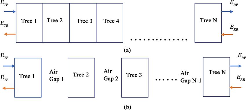
S. Peden et al.
2η1 2 ε c0
=t01 = , (4)
η0 + η1 ε c1 + ε c 0
2η0 2 ε c1
=t10 = , (5)
η0 + η1 ε c1 + ε c 0
where, η0 and η1 are the intrinsic impedances of air and the first lossy medium
respectively, and εc0 is the relative permittivity of air (=1).
Converting the S-parameter matrix to T-parameter matrix [34], Equation (1)
can be written as
1 Γ 01
t01 E1R
ETR t01
E = −Γ . (6)
TF 10 1 E1F
t
01 t01
2.1.2. Second Two-Port Network
The output electric field phasor, E1F of first two-port network travels through the
first lossy medium and comes out of the medium attenuated as E2F. Similarly, E2R
enters the lossy medium and exits attenuated as E1R. The S-parameter for this
two-port network can be written as
E1R 0 e −γ1d1 E1F
E = −γ1d1 , (7)
2 F e 0 E2 R
where, γ1 is the complex propagation constant of the first lossy medium. Com-
plex propagation constant of a sinusoidal electromagnetic wave is a measure of
the change undergone by the amplitude and phase of the wave as it propagates
in a given direction. The real part of γ is the attenuation constant, α in Np/m
(Nepers per m) and the imaginary part is the phase constant, β in rad/m [35].
The complex propagation constant can be expressed as [35]:
γ 1 = jω µ0ε 0ε c1 , (8)
where, ε0 and µ0 are the permittivity and permeability of vacuum respectively, ω
is the angular frequency in rad/sec and εc1 is the complex permittivity of the first
lossy medium. Complex permittivity, εc1 is expressed as
ε=
c1 ε c′1 − jε c′′1 , (9)
where, the real part, ε c′1 represents the relative permittivity and the imaginary
part, ε c′′1 represents the dielectric loss [30].
Converting the S-parameter matrix to T-parameter matrix, Equation (7) can
be written as
E1R e −γ 1d1 0 E2 R
E = γ 1d1 . (10)
1F 0 e E2 F
The output electric field phasor, E2F of second two-port network transmits
through the second interface, travels through the second lossy medium and it
continues until it transmits into the air through the last interface, which is the
DOI: 10.4236/jemaa.2021.136006 88 Journal of Electromagnetic Analysis and ApplicationsS. Peden et al.
seventh two-port network as per Figure 3.
The electric field phasor on the left-hand side of the cascaded 7 two-port net-
works can be written as simple multiplication of the T-parameter matrices and
the electric field phasor on the right-hand side as
1 Γ 01 1 Γ12
t12 e −γ 2 d2
ETR t01 t01 e
− γ 1d1
0 t12 0
E = −Γ γ 1d1
TF 10 1 0 e −Γ 21 1 0 γ 2 d2
e
t01 t01 t12 t12
(11)
1 Γ 23 1 Γ34
t
t23 e t34 ERR
− γ 3 d3
0 t34
×
23
−Γ32
1 0 eγ 3d3 −Γ 43 1 ERF
t23 t23 t34 t34
where the incident wave at the rightmost interface ERR = 0. If there are N number
of lossy media then Equation (11) can be written as
1 Γ 01 1 Γ N −1, N
ETR ERF t01 t01 e −γ1d1
0 t N −1, N t N −1, N
E = γ 1d1
TF ERF −Γ10 1 0 e −Γ N , N −1 1
t01 t01 t N −1, N t N −1, N
(12)
1 Γ N , N +1
e −γ N d N t
0 N , N +1 t N , N +1 0
×
0 eγ N d N −Γ N +1, N 1 1
t N , N +1 t N , N +1
Then the total loss for N lossy homogenous slabs in dB is
ETF
Lslab = 20 log10 . (13)
ERF
Equation (12) in this paper simplifies to Equation (7) in Peden, et al. [33], in
the special case of N = 1 medium.
2.2. Complex Permittivity of a Tree Canopy
If the lossy homogenous medium mentioned in Section 2.1 is a tree canopy, then
the permittivity εc in Equation (8) and (9) is the permittivity of a tree canopy. A
canopy of a tree consists of leaves, branches/twigs and air, and all these will con-
tribute to the total permittivity of a tree canopy given by,
ε c vv ε v + va ε a ,
= (14)
where, εv and εa are the permittivity of the vegetation (leaves and
branches/twigs) and air in the canopy respectively. vv and va are the volume frac-
tions of the vegetation and air in the canopy envelope respectively.
Ulaby and El-Rayes [32] developed a dielectric model to calculate the dielec-
tric constant of vegetation. They modelled the dielectric constant of vegetation,
εv as a simple addition of three components: a nondispersive residual component
DOI: 10.4236/jemaa.2021.136006 89 Journal of Electromagnetic Analysis and ApplicationsS. Peden et al.
(εr), free-water component (vfwεf) and the bulk vegetation-bound water compo-
nent (vbεb), expressed as
ε v =+
ε r v fwε f + vbε b , (15)
where, vfw is the volume fraction of free water, εf is the dielectric constant of free
water, vb is the volume fraction of the bulk vegetation-bound water mixture and
εb is its dielectric constant. Assuming that εr is a nondispersive residual compo-
nent is supported by Hasted [30] who states that the dielectric loss of many dry
materials is low in the microwave band, having values between 10−1 and 10−3.
Free water may contain dissolved salt and the frequency dependent dielectric
constant of bulk saline water is given by the Debye equation [36],
ε fs − ε f ∞ σ
ε f =ε ′f − jε ′′f =ε f ∞ + −j , (16)
f 2πf ε 0
1+ j
ff0
where, f is the operating frequency in Hz, ff0 is the relaxation frequency in Hz,
and εfs and εf∞ are the dimensionless static and high frequency limits of ε ′f . The
salinity, S of a solution is defined as the total mass of salt in grams dissolved in a
solution of 1 kg and is expressed as parts per thousand on a weight basis. The sa-
linity for vegetation is taken to be 10‰ [37]. For salinity, S ≤ 10‰ and at room
temperature, Equation (16) could be approximated as,
75 σ 18
ε f =+
4.9 −j , (17)
f f
1+ j
18
where, f is in GHz. The conductivity σ (siemen/metre) may be related to S (‰)
by,
σ ≅ 0.16S − 0.0013S 2 . (18)
For bound water, Ulaby and El-Rayes [32] conducted dielectric measurements
on sucrose-water mixture and data was fitted to Cole-Cole dispersion equation.
The complex dielectric constant of bound water is given by
55
ε=
b 2.9 + 0.5
, (19)
jf
1+
0.18
where, f is in GHz. Equation (17) includes a loss term associated with the conduc-
tivity of the free water and dissolved ions in the medium. In contrast, Equation
(19) has no corresponding conductivity term as the water molecules are bound to
other substances and do not contribute to bulk conductivity of the medium.
By inserting Equations (17) and (19) in Equation (15), the dielectric constant
of a vegetation can be written as
75 σ 18 55
εv =
ε r + v fw 4.9 + −j + vb 2.9 + .
(20)
f f jf
0.5
1+ j
18 1 +
0.18
DOI: 10.4236/jemaa.2021.136006 90 Journal of Electromagnetic Analysis and ApplicationsS. Peden et al.
The variation of εr, vfw and vb with gravimetric moisture content, Mg were de-
rived by Ulaby and El-Rayes [32] by fitting their model (Equation (20)) to com-
plex permittivity measurements acquired using corn leaves and verified against
corn stalks, soybean leaves, aspen leaves, balsam fir trunk, potatoes, apples, and
other types of vegetation material. The empirical equations are as follows:
εr =
1.7 − 0.74 M g + 6.16 M g2 , (21)
=v fw M g ( 0.55M g − 0.076 ) , (22)
4.64 M g2
vb = , (23)
1 + 7.36 M g2
where, Mg is calculated from the weight measurement of tree before and after
drying as follows
weight of dry tree
M g = 1 − . (24)
weight of tree ( different stages of drying )
By inserting Equation (20) in Equation (14), the dielectric constant of a tree
canopy can be written as
75 σ 18 55
ε c = ε r + v fw 4.9 + −j +
b v 2.9 +
0.5
× v
v + va ε a . (25)
f f jf
1+ j 1+
18 0.18
3. Material and Method
3.1. Experimental Site and Equipment Used
All the experiments were conducted in an indoor facility at The University of
New England main campus located in Armidale, New South Wales, Australia.
Two flat-panel, phased-array directional antennas (ARC Wireless Solutions,
USA, PA2419B01, 39.1 cm × 39.1 cm × 4.3 cm) were used, one as a transmitter
connected to a transceiver Beacon (Dosec Design, Australia, EnviroNode Bea-
con) and the other as a receiver connected to a transceiver hub (Dosec Design,
Australia, EnviroNode Hub) operated at a frequency of 2.4331 GHz. The an-
tenna had a gain of 19 dBi, front-to-back ratio of >30 dB and 3 dB beamwidth of
±9˚. The antennas were placed facing each other at a separation of 6.15 metres.
A constant transmitted power of 100 milliwatts was used. The hub measured and
logged the RSSI (received signal strength indicator, dBm) to a removable SD
card at 1-minute intervals. The experimental set-up is shown in Figure 4.
A Eucalyptus blakelyi (also known as Blakely’s red gum) tree about 2.6 m in
height (Tree 1) was cut and was mounted on a wooden pallet. The RSSI (dBm)
for no obstruction between the transceivers was measured for 4 minutes and
then the tree was placed in front of one antenna. The difference between the
time-average RSSI with and without the tree in place was converted to a
time-averaged RF loss associated with the tree. The sequence of tree and no tree
DOI: 10.4236/jemaa.2021.136006 91 Journal of Electromagnetic Analysis and ApplicationsS. Peden et al.
Figure 4. Experimental set-up within the indoor facility. Two flat-panel antennas were
mounted facing each other 6.15 m apart. A tree was placed immediately in front of one
antenna. The RSSI (dBm) was recorded to a removable SD card inside the transceiver
Hub every minute. The tree canopy can be approximated as an ellipse (black annotation).
measurements was repeated three times to provide a measurement average. The
RF loss (L) associated with the tree canopy was then calculated using,
L ( dB ) RSSI ( no tree ) − RSSI ( tree ) .
= (26)
Following the RSSI measurements with and without the tree in place, the tree
was left to dry for one hour and the measurement RF loss was repeated.
The process of drying and remeasuring the RSSI was repeated until no further
weight loss from drying was achieved (i.e. tree was considered dry). At this end
point the mass of the water (mw) in the tree canopy and subsequently each par-
tially-dried tree canopy was retrospectively calculated from the known mass of
the tree during drying and the final dry weight of the tree.
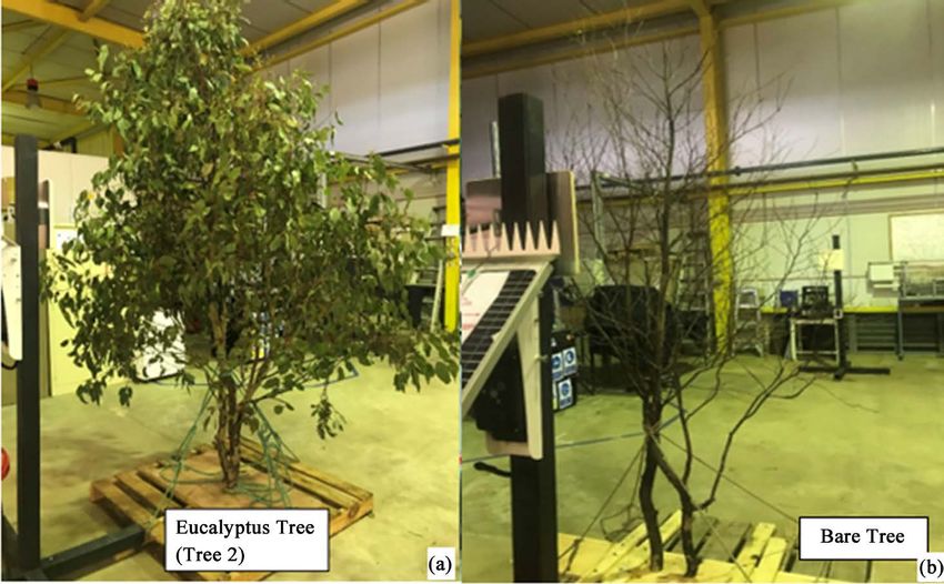
The measurement sequence was repeated for another tree with leaves (Tree 2)
and a third, bare tree without leaves (Bare tree) as shown in Figure 5. Note that
the bare tree was left to dry for a day rather than an hour before the measure-
ment was repeated. The measurement sequence was also repeated for two trees
positioned in series as shown in Figure 6.
3.2. Calculation of Volume Fractions
The tree canopy was considered as an ellipsoid (refer Figure 4) and the volume
of the tree canopy envelope was calculated as follows
π
V= × A× B × C , (27)
6
where, A, B and C are the lengths of the principal axes and these lengths were
measured using a measuring tape for each tree. A, B and C of the trees used for
DOI: 10.4236/jemaa.2021.136006 92 Journal of Electromagnetic Analysis and ApplicationsS. Peden et al.
the experiments are listed in Table 1.
Figure 5. (a) Tree 2 with leaves and (b) Bare tree positioned in between the transceivers.
Figure 6. Two trees (Tree 1, Tree 2) positioned in series in between the transceivers.
Table 1. Dimensions of a tree to calculate the volume of the tree. The tree canopy was
considered as an ellipsoid and A, B and C are the three lengths of the principle axes of an
ellipsoid in metres.
Eucalyptus Tree A (m) B (m) C (m)
1 Tree 1 with leaves 1.30 1.70 2.10
2 Tree 2 with leaves 1.55 1.80 2.15
3 Bare tree 1.36 1.40 2.10
DOI: 10.4236/jemaa.2021.136006 93 Journal of Electromagnetic Analysis and ApplicationsS. Peden et al.
The volume fraction of vegetation, vv is a summation of volume fraction of the
leaves in the canopy, vL and the volume fraction of the woody part (branches) in
the canopy, vwood are given by,
v=
v vL + vwood , (28)
vL = VL V , (29)
vwood = Vwood V , (30)
where, VL and Vwood are the volume of leaves and woody part of the canopy re-
spectively. Then the volume fraction of air, va is given by
va = 1 − vv . (31)
The volume of leaves and woody part of the canopy are calculated using their
mass and density as shown below
VL = mL ρ L , (32)
Vwood = mwood ρ wood , (33)
where mL and mwood are the weight of the leaves and woody part in the canopy
respectively. The leaves were taken off from the (third) tree and weighed, and
the tree was weighed separately in order to yield the values for mL and mwood. The
densities of the leaves, ρL = 876 kg/m3 and woody parts, ρwood = 1110 kg/m3 were
determined from the measurements of weight and volume of fresh leaves and
fresh woody parts respectively. The volume was measured using a displacement
method in water. An assumption was made here that the leaves do not shrink
when the tree canopy dries out and the volume remains the same throughout the
measurement period.
3.3. Calculation of Effective Water Path (EWP)
The radio wave passes through a tree with vegetation thickness, d containing a
distributed mass, mw of water (kg), we introduce the effective water path (EWP)
in mm expressed as
m ×d
EWP w
= × 1000 , (34)
ρw ×V
where, V is the volume of the tree canopy envelope in m3 (refer Equation (27)),
ρw is the density of pure water (1000 kg/m3) and d in our experiment is equal to
the dimension A mentioned in Table 1.
For N number of trees, EWP is a summation of EWP of each tree as follows
= EWP1 + EWP2 + EWP3 + + EWPN .
EWP (35)
4. Results and Discussion
The measured 2.4 GHz RF loss through the tree canopies for Tree 1, Tree 2, Bare
tree (after leaves were removed by hand) and Trees 1 and 2 in series are depicted
in Figure 7. The RF loss in dB is maximum when the leaves are fresh and the RF
loss trends down with the reduction of EWP associated with drying. The modelled
DOI: 10.4236/jemaa.2021.136006 94 Journal of Electromagnetic Analysis and ApplicationsS. Peden et al. DOI: 10.4236/jemaa.2021.136006 95 Journal of Electromagnetic Analysis and Applications
S. Peden et al.

                                 Figure 7. Plots of measured and modelled (Equation (13)) RF loss (dB) as functions of
                                 EWP (mm) for Eucalyptus blakelyi trees ((a) Tree 1; (b) Tree 2; (c) Bare tree; (d) Trees 1
                                 & 2 in series).

                                 values of the RF loss versus EWP (Equation (13)) is also depicted in the graphs
                                 of Figure 7 (red curves).
                                   The volume fractions were calculated using the equations mentioned in Sec-
                                 tion 3.2. The tree canopy consisted of 0.6% vegetation (vv) and the remainder is
                                 air (va). The vegetation (0.6%) subdivides to 0.2% leaves (vL) and 0.4% woody
                                 parts (vwood) of the tree canopy. For the bare tree, vL = 0%, vwood = 0.4% and the
                                 remainder is air. An assumption here was made that these volume fractions re-
                                 main unchanged throughout the experimental period.
                                   The measured RF loss is generally higher than modelled in all the cases shown
                                 in Figure 7 irrespective of whether the tree canopy had leaves or not, or whether
                                 there was a single tree or two trees in series in between the transceivers. The
                                 consistent offset between the measured and modelled values, we believe, is at-
                                 tributable to not adequately accounting for the residual water in estimating EWP
                                 using Equation (34). The method we used to dry the leaves may not have re-
                                 moved the water completely, especially the bound water [30] [31]. When dried
                                 to a constant weight, vegetation is in an equilibrium state with the drying air
                                 [31]. Moreover, the tree may then re-absorb water from the air when the ex-
                                 periment was being carried out.
                                   Quantifying the bound water in leaves, on the other hand, is difficult although
                                 it can be estimated using a calorimetric methodology [38] [39] [40]. Note this
                                 methodology refers to the notion of unbound and bound water as being, respec-
                                 tively, “freezable” and “unfreezable”. Assuming they are related, we were unable
                                 to discern this value for eucalyptus leaves using available literature. However,
                                 Whitman [41] provides an insight into at least the possible orders of magnitude
                                 of this value on the basis of his work on a range of Prairie grasses in the U.S.
                                 during the summer season. Sagebrush, for example, has a bound water content

DOI: 10.4236/jemaa.2021.136006                          96            Journal of Electromagnetic Analysis and Applications
S. Peden et al. DOI: 10.4236/jemaa.2021.136006 97 Journal of Electromagnetic Analysis and Applications
S. Peden et al.

                                 Figure 8. Plots of measured and modelled (Equation (13) with additional water content
                                 of 13%) RF loss (dB) as functions of EWP (mm) for Eucalyptus blakelyi trees ((a) Tree 1,
                                 (b) Tree 2; (c) Bare tree; (d) Trees 1 & 2 in series).

                                 in its leaves ranging from 10% - 30% (dry-weight basis) with other grass species
                                 exhibiting similar ranges and sometimes higher. In this earlier work, however,
                                 the bound water content is measured from freshly-sourced leaves which were
                                 not subjected to further desiccation. Here the values would be influenced by ex-
                                 ternal factors such as soil moisture content, etc. [41].
                                   An empirical approach available in this work is to identify the value of bound
                                 water that would elevate the modelled data values in Figure 7 to the measured
                                 values, effectively considering the actual water content of our trees to be higher
                                 (by this additional, bound contribution). We identified this value by finding the
                                 minimum total variance between measured and modelled values. To this end,
                                 the residual water was varied from 1% to 25% in 0.1% increments. The best fit
                                 between the modelled and the measured values is achieved by assuming that the
                                 tree canopies contained an additional water content of 13% when dried to con-
                                 stant weight. Residual water of this order of magnitude is plausible when com-
                                 pared against measurements of other leaf types [41]. Of course, what remains
                                 unclear is whether or not the “unfreezable” and “freezable” components of water
                                 identified by Whitman and others [38] [39] [40] is accessible through the leaf
                                 desiccation process in this work (or not) and whether the bound component is a
                                 contributor to the RF losses observed in this work.
                                   Nevertheless, and with the new adjustment in the dry weight, the offset be-
                                 tween the modelled and measured data collapses (refer Figure 8), reducing the
                                 RMSE by 31% - 42% compared to the unadjusted model.

                                 5. Conclusions
                                 A plane wave model, including an estimation of the bound water content of tree

DOI: 10.4236/jemaa.2021.136006                         98            Journal of Electromagnetic Analysis and Applications
S. Peden et al.
canopies, was developed to calculate the RF loss through eucalyptus tree canopy
as a function of EWP at a frequency of 2.4 GHz. There was a positive non-linear
relationship between RF loss in dB and the water content of the tree when the
latter is expressed as EWP in mm. When the model was adjusted for additional
water content of 13%, EWP was found to explain 66% and 90% of the variance
in the observed RF loss for single tree canopies with leaves and single tree with-
out leaves respectively. It was also found to explain 75% of the variance when
two trees with leaves were positioned in series.
The model developed in this research is compared against eucalyptus leaves
and trees of some species. To generalize this model for wide range of tree types,
the model needs to be compared against experiments acquired using other types
of trees and other species of Eucalyptus. Verification of the model could also be
done by using other parts of the tree as the lossy medium.
Acknowledgements
The first author acknowledges receipt of a Tuition Fee-Wavier Scholarship from
the University of New England. One of us (DWL) acknowledges the support of
Food Agility CRC Ltd, funded under the Commonwealth Government CRC
Program. The CRC Program supports industry-led collaborations between in-
dustry, researchers, and the community. All authors gratefully acknowledge the
contribution of Derek Schneider and Antony McKinnon from UNE for their
help in setting up the experiment, and Prof. Jeremy Bruhl from UNE for helping
us identify the eucalyptus species used for the experiment.
Conflicts of Interest
The authors declare no conflicts of interest regarding the publication of this pa-
per.
References
[1] Boland, D.J., et al. (2006) Forest Trees of Australia. 5th Edition, Victoria CSIRO
Publishing, Victoria.
[2] Matusick, G., Ruthrof, K., Brouwers, N., Dell, B. and Hardy, G. (2013) Sudden For-
est Canopy Collapse Corresponding with Extreme Drought and Heat in a Mediter-
ranean-Type Eucalypt Forest in Southwestern Australia. European Journal of Forest
Research, 132, 497-510. https://doi.org/10.1007/s10342-013-0690-5
[3] ABARES (2018) Australia’s State of the Forests Report. Department of Agriculture
and Water Resources, Australia.
[4] Allen, C.D., et al. (2010) A Global Overview of Drought and Heat-Induced Tree
Mortality Reveals Emerging Climate Change Risks for Forests. Forest Ecology and
Management, 259, 660-684. https://doi.org/10.1016/j.foreco.2009.09.001
[5] Belyazid, S. and Giuliana, Z. (2019) Water Limitation Can Negate the Effect of
Higher Temperatures on Forest Carbon Sequestration. European Journal of Forest
Research, 138, 287-297. https://doi.org/10.1007/s10342-019-01168-4
[6] Kirkham, M.B. (2016) Elevated Carbon Dioxide: Impacts on Soil and Plant Water
Relations. CRC Press, Boca Raton. https://doi.org/10.1201/b10812
DOI: 10.4236/jemaa.2021.136006 99 Journal of Electromagnetic Analysis and ApplicationsS. Peden et al.
[7] Osakabe, Y., Osakabe, K., Shinozaki, K. and Tran, L.S. (2014) Response of Plants to
Water Stress. Frontiers in Plant Science, 5, 86.
https://doi.org/10.3389/fpls.2014.00086
[8] Pallardy, S., Pereira, J. and Parker, W. (1991) Measuring the State of Water in Tree
Systems. In: Lassoie, J.P. and Hinckley, T.M., Eds., Techniques and Approaches in
Forest Tree Ecophysiology, CRC Press, Boca Raton, 28-76.
[9] Pereira, J. and Pallardy, S. (1989) Water Stress Limitations to Tree Productivity. In:
Biomass Production by Fast-Growing Trees, Springer, Berlin, 37-56.
https://doi.org/10.1007/978-94-009-2348-5_3
[10] Zhou, J., Zhou, J., Ye, H., Ali, M.L., Nguyen, H.T. and Chen, P. (2020) Classification
of Soybean Leaf Wilting Due to Drought Stress Using UAV-Based Imagery. Com-
puters and Electronics in Agriculture, 175, Article ID: 105576.
https://doi.org/10.1016/j.compag.2020.105576
[11] Resh, H.M. (2015) Signs of Plant Nutritional and Physiological Disorders and Their
Remedies. In: Hydroponics for the Home Grower, CRC Press, Boca Raton, 76-89.
https://doi.org/10.1201/b18069-16
[12] Peñuelas, J., Filella, I., Serrano, L. and Save, R. (1996) Cell Wall Elasticity and Water
Index (R970 nm/R900 nm) in Wheat under Different Nitrogen Availabilities. In-
ternational Journal of Remote Sensing, 17, 373-382.
https://doi.org/10.1080/01431169608949012
[13] Peñuelas, J., Filella, I., Biel, C., Serrano, L. and Save, R. (1993) The Reflectance at the
950-970 nm Region as an Indicator of Plant Water Status. International Journal of
Remote Sensing, 14, 1887-1905. https://doi.org/10.1080/01431169308954010
[14] Datt, B. (1999) Remote Sensing of Water Content in Eucalyptus Leaves. Australian
Journal of Botany, 47, 909-923. https://doi.org/10.1071/BT98042
[15] LaGrone, A.H. (1960) Forecasting Television Service Fields. Proceedings of the IRE,
48, 1009-1015. https://doi.org/10.1109/JRPROC.1960.287501
[16] Balachander, D., Rao, T.R. and Mahesh, G. (2013) RF Propagation Experiments in
Agricultural Fields and Gardens for Wireless Sensor Communications. Progress in
Electromagnetics Research C, 39, 103-118. https://doi.org/10.2528/PIERC13030710
[17] Hristos, T.A., et al. (2014) A Computational Model for Path Loss in Wireless Sensor
Networks in Orchard Environments. Sensors, 14, 5118-5135.
https://doi.org/10.3390/s140305118
[18] Weissberger, M.A. (1982) An Initial Critical Summary of Models for Predicting the
Attenuation of Radio Waves by Trees.
[19] Seville, A. and Craig, K. (1995) Semi-Empirical Model for Millimetre-Wave Vegeta-
tion Attenuation Rates. Electronics Letters, 31, 1507-1508.
https://doi.org/10.1049/el:19951000
[20] Al-Nuaimi, M.O. and Stephens, R.B.L. (1998) Measurements and Prediction Model
Optimisation for Signal Attenuation in Vegetation Media at Centimetre Wave Fre-
quencies. IEE Proceedings—Microwaves, Antennas and Propagation, 145, 201-206.
https://doi.org/10.1049/ip-map:19981883
[21] Adegoke, A.S. (2014) Measurement of Propagation Loss in Trees at SHF Frequen-
cies. Ph.D. Thesis, Department of Engineering, University of Leicester, Leicester.
[22] Guo, X.-M. and Zhao, C. (2014) Propagation Model for 2.4 GHz Wireless Sensor
Network in Four-Year-Old Young Apple Orchard. International Journal of Agri-
cultural and Biological Engineering, 7, 47-53.
[23] Rogers, N.C., et al. (2002) A Generic Model of 1-60 GHz Radio Propagation through
DOI: 10.4236/jemaa.2021.136006 100 Journal of Electromagnetic Analysis and ApplicationsS. Peden et al.
Vegetation—Final Report. Radio Agency, UK.
[24] Jiang, S. and Georgakopoulos, S. (2011) Electromagnetic Wave Propagation into
Fresh Water. Journal of Electromagnetic Analysis and Applications, 3, 261-266.
https://doi.org/10.4236/jemaa.2011.37042
[25] Da Silva, M.J. (2008) Impedance Sensors for Fast Multiphase Flow Measurement
and Imaging. Ph.D. Thesis, Electrical and Computer Engineering Department, Tech-
nische Universität Dresden, Dresden.
[26] Lunkenheimer, P., et al. (2017) Electromagnetic-Radiation Absorption by Water.
Physical Review E, 96, Article ID: 062607.
https://doi.org/10.1103/PhysRevE.96.062607
[27] Le Vine, D.M. and Karam, M.A. (1996) Dependence of Attenuation in a Vegetation
Canopy on Frequency and Plant Water Content. IEEE Transactions on Geoscience
and Remote Sensing, 34, 1090-1096. https://doi.org/10.1109/36.536525
[28] Nakajima, I., Ohyama, F., Juzoji, H. and Ta, M. (2019) Developing a Scanner for
Assessing Foliage Moisture. Journal of Multimedia Information System, 6, 155-164.
https://doi.org/10.33851/JMIS.2019.6.3.155
[29] Shmulsky, R. and Jones, P.D. (2011) Wood and Water. In: Forest Products and Wood
Science: An Introduction, 6th Edition, John Wiley & Sons, Hoboken, 141-174.
https://doi.org/10.1002/9780470960035.ch7
[30] Hasted, J.B. (1973) Aqueous Dielectrics. Chapman and Hall Ltd., London.
[31] Yang, W. and Siebenmorgen, T. (2003) Drying Theory. In: Encyclopedia of Agri-
cultural, Food, and Biological Engineering, Marcel Dekker, New York, 231-241.
[32] Ulaby, F.T. and El-Rayes, M.A. (1987) Microwave Dielectric Spectrum of Vegeta-
tion Part II: Dual-Dispersion Model. IEEE Transactions on Geoscience and Remote
Sensing, GE-25, 550-557. https://doi.org/10.1109/TGRS.1987.289833
[33] Peden, S., Bradbury, R.C., Lamb, D.W. and Hedley, M. (2021) A Model for RF Loss
through Vegetation with Varying Water Content. Journal of Electromagnetic Anal-
ysis and Applications, 13, 41-56. https://doi.org/10.4236/jemaa.2021.133003
[34] Frickey, D.A. (1994) Conversions between S, Z, Y, H, ABCD, and T Parameters
Which Are Valid for Complex Source and Load Impedances. IEEE Transactions on
Microwave Theory and Techniques, 42, 205-211. https://doi.org/10.1109/22.275248
[35] Balanis, C.A. (2012) Advanced Engineering Electromagnetics. John Wiley & Sons,
Hoboken.
[36] Ulaby, F.T., Moore, R.K. and Fung, A.K. (1986) Microwave Remote Sensing: Active
and Passive. Volume 3 From Theory to Applications. Artech House, Norwood.
[37] El-Rayes, M.A. (1987) The Measurement and Modeling of the Dielectric Behavior of
Vegetation Materials in the Microwave Region (0.5-20.4 GHZ). Ph.D. Thesis, De-
partment of Electrical and Computer Engineering, University of Kansas, Lawrence.
[38] Robinson, W. (1931) Free and Bound Water Determinations by the Heat of Fusion
of Ice Method. Journal of Biological Chemistry, 92, 699-709.
https://doi.org/10.1016/S0021-9258(17)32613-3
[39] Sayre, J.D. (1932) Methods of Determining Bound Water in Plant Tissue. Journal of
Agricultural Research, 44, 669-688.
[40] Stark, A.L. (1932) An Apparatus and Method for Determining Bound Water in Plant
Tissue. Proceedings of the American Society for Horticultural Science, 29, 384-388.
[41] Whitman, W.C. (1941) Seasonal Changes in Bound Water Content of Some Prairie
Grasses. Botanical Gazette, 103, 38-63. https://doi.org/10.1086/335024
DOI: 10.4236/jemaa.2021.136006 101 Journal of Electromagnetic Analysis and ApplicationsYou can also read