Revised Model of Abrasive Water Jet Cutting for Industrial Use
←
→
Page content transcription
If your browser does not render page correctly, please read the page content below
materials
Article
Revised Model of Abrasive Water Jet Cutting for Industrial Use
Libor M. Hlaváč

                                          Department of Physics, VSB–Technical University of Ostrava, 17. listopadu 15/2172,
                                          708 00 Ostrava, Czech Republic; libor.hlavac@vsb.cz; Tel.: +420-59-732-3102

                                          Abstract: Research performed by the author in the last decade led him to a revision of his older
                                          analytical models used for a description and evaluation of abrasive water jet (AWJ) cutting. The
                                          review has shown that the power of 1.5 selected for the traverse speed thirty years ago was influ-
                                          enced by the precision of measuring devices. Therefore, the correlation of results calculated from a
                                          theoretical model with the results of experiments performed then led to an increasing of the traverse
                                          speed exponent above the value derived from the theoretical base. Contemporary measurements,
                                          with more precise devices, show that the power suitable for the traverse speed is essentially the
                                          same as the value derived in the theoretical description, i.e., it is equal to “one”. Simultaneously, the
                                          replacement of the diameter of the water nozzle (orifice) by the focusing (abrasive) tube diameter
                                          in the respective equations has been discussed, because this factor is very important for the AWJ
                                          machining. Some applications of the revised model are presented and discussed, particularly the
                                          reduced forms for a quick recalculation of the changed conditions. The correlation seems to be very
                                          good for the results calculated from the present model and those determined from experiments. The
                                          improved model shows potential to be a significant tool for preparation of the control software with
                                          higher precision in determination of results and higher calculation speed.

                                Keywords: abrasive water jet; modelling; cutting; process control; industrial application


Citation: Hlaváč, L.M. Revised
Model of Abrasive Water Jet Cutting
for Industrial Use. Materials 2021, 14,   1. Introduction
4032. https://doi.org/10.3390/ma
                                                The period of extensive use of water jet and abrasive water jet industrial application
14144032
                                          started more than 50 years ago. The first models for water jets were presented in the
                                          1970s [1,2]. During the 1980s, Hashish presented his studies of abrasive water jets [3,4].
Academic Editor: Pawel Pawlus
                                          More recently, in the beginning of the 1990s, Hlaváč presented his theoretical model pre-
Received: 25 June 2021
                                          pared for both water and abrasive water jets [5]. Later on, during the 1990s and in the
Accepted: 16 July 2021                    beginning of the 21st century, many researchers all over the world continued modelling ac-
Published: 19 July 2021                   tivities aimed at abrasive water jet machining. Regression-based models were prepared [6]
                                          and the first models for 3D machining were published [7,8]. Models aimed at including
Publisher’s Note: MDPI stays neutral      inherent phenomena have been prepared, namely, those describing processes in the mixing
with regard to jurisdictional claims in   chamber and the focusing tube [9], in the interaction area [10,11] and some geometrical
published maps and institutional affil-   phenomena of the cutting processes. The research teams focused on processes with sub-
iations.                                  stantial impact on product geometry: origin of the cutting surface [12–14], formation of
                                          the striations [15–17] and the taper [18,19], determination of the jet lag inside kerf [20] and
                                          influence of the cutting parameters on the kerf geometry [21,22].
                                                In recent years, many specific research applications have grown in importance. First
Copyright: © 2021 by the author.
                                          of all, there are investigations aimed at some specific materials like thick metals [23] and
Licensee MDPI, Basel, Switzerland.        titanium alloys for aerospace [24,25]. Some other interesting materials are glass [26] or
This article is an open access article    composites [27]. Very interesting research was performed by Akkurt [28], who studied
distributed under the terms and           the front characteristics in applications of the AWJ on brass. Some recent investigations
conditions of the Creative Commons        focused on a suppression of the negative impact of the trailback and the taper on the
Attribution (CC BY) license (https://     product quality [29], namely, in machining of composites [30,31]. Other researchers focus
creativecommons.org/licenses/by/          on various mathematical—numerical methods and their applications in AWJ processes.
4.0/).

Materials 2021, 14, 4032. https://doi.org/10.3390/ma14144032                                               https://www.mdpi.com/journal/materials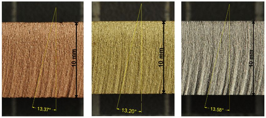
Materials 2021, 14, 4032                                                                                            2 of 16

                           These methods are, namely, finite element methods (FEM) [32,33], smoothed particle
                           hydrodynamics (SPH) [34] and computational fluid dynamics (CFD) [35].
                                The investigation of AWJ machining cannot be adequate without research of abrasive
                           materials. Some researchers focused on investigations of the disintegration of abrasive
                           particles in the mixing process [36], others searched for new types of abrasive materials [37],
                           others studied the recycled ones [38,39] or try to apply ice particles [40], as the most
                           environmentally friendly abrasive. Some special applications like using the AWJ for
                           sculpturing [41], micro-piercing [42] or micro-machining [43] bring new challenges for
                           researchers dealing with water jetting. However, the studies of applications of AWJ on
                           the “classical” materials like tiles [44], wood [45] or Hardox [46] can also bring about
                           new knowledge. The problem of surface quality is often closely tied in with the surface
                           roughness. Therefore, many investigations were performed to assess, predict or monitor
                           this parameter [47–50]. A few publications were also addressed at the reliability and safety
                           problems of water jet technologies [51] or other related problems. However, preparation of
                           the theoretical and more complex models is quite rare in the last decade. Therefore, partial
                           models focused on either the mixing processes [52], modelling of the abrasive particles
                           energy [53], or on the preparation of some superstructures for previous models [54,55],
                           or in combination, have been presented. Recent research effort is focused on numerical
                           modelling of abrasive water jets, e.g., the impact on material and the respective kerf
                           shapes [56] or modelling of the micro-machining process imprint shapes [57]. However,
                           the upgraded analytical model of the abrasive water jet that is presented in this article can
                           be a new direction for the innovation of control systems for abrasive water jetting facilities
                           and the development of some new devices, improved software systems, or in combination.

                           2. Plain Waterjet—Material Interaction: Summary of the Initial Physical Model
                                The model of water jet (WJ) interaction with material has been derived by applying the
                           analytical physical description of the interaction process and it was presented in [58]. The
                           derivation of this initial model was based on application of basic physical principles—the
                           energy conservation law and the momentum conservation law. The resulting two equations
                           are necessary for a development of the subsequent abrasive water jet model. Therefore, the
                           most important forms presented in [58] are summarized here:
                                                                q
                                                                                        ∗ ∗
                                                         π do  2ρo µ3 γ3p p3o e−5(ξ L + ξ hn ) (1 − α2n ) cos θ
                                             h n +1   =            ρo                                                (1)
                                                                                        ∗ ∗
                                                        8 χ ρ M vePM α2n e−2(ξ L + ξ hn ) µ γ p po + ρ Mo σ
                                                                  ρ                                      ρ

                                                                         q
                                                                      C2f 2µ3 γ3p p3o ρ∗M k∗
                                                          αn    = 1 − √                    ∗ ∗                         (2)
                                                                     8 ρo η σs a e3(ξ L + ξ hn )
                                                       h∗n = h1 + h2 + h3 + . . . + hn−1 + hn                          (3)
                                The first equation describes the depths of penetration of the pure water jet into a
                           material in the (n + 1)-th pass along the same trace. The axis of the impinging jet is tilted
                           from the perpendicular to the surface in the “plane of cut” for the angle θ. The “plane
                           of cut” is determined by the traverse speed vector and the jet axis. The second equation
                           calculates the energy absorption coefficient α after the n-th pass of the jet along the same
                           trace. The third equation summarizes the penetrations of the individual passes to the
                           total depth of penetration. The equations have been used in the expression for one pass
                           and without tilting for the basic preparation of the AWJ model through the principles of
Materials 2021, 14, 4032 3 of 16
similarity. Therefore, the AWJ derivation starts from the application of these two equations
for calculations of the pure water jet’s impact on materials:
q
π do 2ρo µ3 γ3p p3o e−5ξ L (1 − α2 )
h = ρo (4)
ρ
vePM α2 e−2ξ L µ γ p po + ρ Mo σ
ρ
8 χ ρM
q
C2f 2µ3 γ3p p3o ρ∗M k∗
α = 1 − √ (5)
8 ρo η σs a e3ξ L
However, several additional specific phenomena typical for AWJ must be introduced
into the model to prepare fairly reliable equations, as is described in the next sections.
3. Differentness in Description of the Abrasive Water Jet Regarding Pure Water Jet
The most important difference between the AWJ and the pure water jet is the presence
of solid-state abrasive particles inside the resulting jet (flow). This contribution is aimed
at the injection AWJ, but some resulting formulas can be applied even for the slurry jets.
Nevertheless, the process of abrasive mixing with the water jet, specific for the injection
jets, needs deeper analysis, because, contrary to the slurry jets, abrasive particles undergo
a substantial size change during the mixing process. The abrasive particle size change has
been studied many times for various purposes in the past, e.g., as a tool for the intended
disintegration of some minerals or coal [59,60]. These studies have shown a substantial
reduction of the particle size in the mixing process. Therefore, the equation for calculation
of the abrasive particle size change needs to be included into the system of equations
applied in the control loop of the cutting system. It can be used in this form (see [59]):
ao
an = (6)
CD πd2o µ2o p2o γo2
1+ 24ρEP ao co c
The next specific parameters modifying efficiency of the AWJ are connected with the
energy losses and the momentum changes inside the mixing chamber and the focusing
tube. To define these phenomena more precisely, Hlaváč introduced four coefficients
modifying velocity of the mixture [9]. The first one modifies velocity according to the
suction capacity when the number of incoming particles exceeds the limit for the proper
mixing and particles acceleration (C1 ):
π ρ a vi a3o 3 qa v
C1 = For ≤ i ⇒ C1 = 1 (7)
3 do q a π ρ a a3o do
The second coefficient (C2 ) indicates smooth flow, as the number of disintegrated
particles passing through the focusing tube cross-section is limited:
da √
C2 = √ For d a > 6 an ⇒ C2 = 1 (8)
6 an
Modification of the velocity due to the friction inside the focusing tube with respect to
the material of the tube indicates coefficient C3 :
C3 = (1 − f la ) (9)
The fourth coefficient (C4 ) modifies the mixture velocity according to the size relations
in the system “orifice diameter—abrasive particle size—focusing tube diameter”. Consid-Materials 2021, 14, 4032 4 of 16
ering the non-zero number of the original sized particles in the mixture and their smooth
flowing through the system, the coefficient C4 can be determined as:
( a o + a n + d o )2
C4 = 1 − for d a > 0 (10)
d2a
Equations (7)–(10) are presented here for better understanding of the final model
preparation. The equations determine the coefficients applied for calculation of the resulting
mixture velocity from the momentum conservation law.
qw
v a = C1 C2 C3 C4 vi (11)
qw + q a
It is evident that Equation (11) is similar to the one already presented in the beginning
of the modelling attempts [61]. It is because it is derived in the same manner, from the
momentum conservation law. The coefficient of momentum transfer efficiency η used by
Hashish in [61] is replaced here by the product of four coefficients being calculated or set
by the logical mathematical operations according to the actual state of the cutting process
variables and the mixing conditions.
4. Model of the AWJ Transformed from the WJ Model
The AWJ model prepared by a direct transformation from the pure water jet model
is based on analogy presumption. It is supposed that by transforming the liquid density
and pressure and using the appropriate quantities in Equations (4) and (5) it is possible to
obtain the equation for the depth of the AWJ penetration into material [9]. The first step is
to determine the density of the mixed flow (water with abrasive)—this is determined by
Equation (12).
4ρ a (qw + q a )
ρj = (12)
πρ a vi d2o + 4q a
The next step is to determine the respective pressure of the mixed flow, i.e., liquid with
the density determined using Equation (12). This pressure is calculated from Equation (13).
1 2
pj = ρv (13)
2 j a
Once these most important quantities are determined, the subsequent substitution is
applied in Equations (4) and (5): ρo → ρ j , µγ p po → p j , ξ → ξ j , α → αe . Other variables,
especially the material properties like the density, the grain size, the strength (both the
compressive/tensile and the shear) remain identical for the AWJ as for the pure water jet.
The only specific characteristic is the permeability (used in the case of the pure water jet),
because it is necessary to select some appropriate property instead for the AWJ cutting,
particularly for steels and other metals, carbons, carbides and other materials with low
water absorption and penetration. The material hardness K (or HV) was selected as the
proper variable for the AWJ machining and the respective equations were transformed into
the forms presented in Equations (14) and (15), see also the citation [14], or Equation (16),
see [55]. The exponent used for the traverse speed (number 1.5 instead of the ratio of the jet
and the cut material densities) has been determined from the regressions of a huge amount
of experimental data obtained on many cut materials in the late 1980s and during the 1990s.
q
C A S p π do 2ρ j p3j e−5ξ j L (1 − α2e )
hlim = (14)
8 (v P + v Pmin )1.5 ρm p j α2e e−2ξ j L + ρ j σm
q
2p3j K ti
α e = 1− √ (15)
8 ρ j σm amMaterials 2021, 14, 4032 5 of 16
q 23
C A SP πd0 2ρ j p3j e−5ξ j L 1 − α2e
v Plim = − v Pmin (16)
2 −2ξ j L
8H ρm p j αe e + ρj σ
Nevertheless, problems with determination of the proper interaction time ti in the
efficiency coefficient αe during the real time calculations in new control software being
prepared in the last few years lead to the repeated detailed analysis of the process. This
analysis uncovered the very important detail. During preparation of the original model of
the AWJ [9] the above-mentioned substitutions were input. Subsequently, the correlation
between experimental data and results calculated from that theory led to the introduction
of the power 1.5 for the traverse speed. All further works were influenced by these
decisions. Nevertheless, the experiments used for correlation were influenced by lower
efficiency of the system generating the AWJ accompanied by the low accuracy of the devices
measuring the pressure inside the high-pressure part of the system. The results were also
influenced by less information about the abrasive material and its disintegration during
the mixing process. All analyses, performed in the last few years, show that exponent
applied at the traverse speed (1.5) is too high and the proper exponent is much closer
to the value resulting from the original theoretical physical derivations, i.e., to “one”.
Therefore, the exponent has been decreased from the value 1.5 to the value “one” (derived
originally from the basic equations for the energy and the momentum conservation laws).
Another possible substitution related to the change from pure water to the abrasive mixture,
do → d a , needs to be largely discussed. Although it seems logical that the focusing tube
diameter should be used instead of the nozzle/orifice diameter, this substitution needs
to be evaluated from the physical point of view. Provided that the diameter of the nozzle
represents the amount of energy delivered to the interaction area, it cannot be replaced
by the focusing tube diameter, because this change does not increase the energy portion
(better said it reduces it). Nevertheless, if the diameter of the nozzle represents the amount
of destroyed material, it could be replaced by the focusing tube diameter. Therefore, the
actual equations for calculation of the jet penetration limit into the material, Equation (17),
or the traverse speed limit for cutting of the selected thickness of material, Equation (18),
have the subsequent forms:
q
CA S p π da 2ρ j p3j e−5ξ j L (1 − α2e )
hlim = (17)
8 (v P + v Pmin ) ρm p j α2e e−2ξ j L + ρ j σm
q
C A SP πd a 2ρ j p3j e−5ξ j L 1 − α2e
v Plim = − v Pmin (18)
8H ρm p j α2e e−2ξ j L + ρ j σ
Supplementary equation for calculation of the efficiency coefficient αe from the cut-
ting process parameters, the material properties and other factors remains unchanged,
commonly expressible in this form:
q
2p3j Kti
αe = 1 − √ (19)
8 ρ j am σs
Equation (17) or Equation (18), together with Equation (19) and, of course, with the
preceding ones, (6)–(13), are directly applicable in practice, both for predictive or analytical
calculations. They can be also used for a preparation of the operating and control software
for machining systems with AWJ (as was proved in the past with their older forms).
Calculation of the coefficient αe is much more convenient in practice from evaluation
of the experimental cut made in material, especially when machining of materials withMaterials 2021, 14, 4032 6 of 16
the untrustworthy material information. The appropriate relation for calculation of the
coefficient αe is then expressed as Equation (20):
v q
C A S p πd a 2ρ j p3j e−5ξ j L − 8h(v P + v Pmin )ρ j σm
u
u
αe = t (20)
u
q
C A S p πd a 2ρ j p3j e−5ξ j L + 8h(v P + v Pmin )ρm p j e−2ξ j L
In the case of machining processes other than cutting, additional equations may be nec-
essary, describing some specific factors and the specific behavior of the jet in the respective
processes. It is also important to add some equations describing the compensation of the
jet delay and the taper during the cutting process [19,55]. The modification of the traverse
speed, for meeting the requirements of a certain surface quality, can be calculated from
Equation (21), introduced, e.g., in [55] and completed by CQ relation to the cut material
behavior and the AWJ abrasive material type; the condition CQ ∈ (0 ; 1i needs to be
fulfilled, because the traverse speed needs to fulfil condition v P ∈ (0 ; v Pmin i .
v PQ = CQ v Plim (21)
Similarly, an analogous equation can be derived for a determination of the depth in
material with a selected quality of the side walls securable at the set traverse speed. How-
ever, the proper relation between the wall quality parameters and the respective traverse
speed and other machining parameters needs further investigation for each material and
its thickness. The values hlim or v Plim are determined from the actual v P and h applying
Equation (22) or Equation (23).
2
ϑlim 3
hlim = h (22)
ϑ
2
ϑlim 3
v Plim = v P (23)
ϑ
Respective declination angles determining the cutting wall quality are calculated from
Equation (24) or Equation (25) within the scope of the jet energy proportionate to the
material thickness.
h 1.5
ϑ = ϑlim (24)
hlim
v P 1.5
ϑ = ϑlim (25)
vlim
The usual angle limit for materials with the thickness correlating with the jet energy
has a value of 45◦ , because both the cutting and the deformation wear of material are
present during the jet–material interaction. However, if the material thickness exceeds
the jet energy capacity, the deformation removal of material (the deformation wear) is
impossible. The jet reflects from the kerf bottom in such a case. Therefore, the angle
limit corresponds to the maximum angle for the cutting mode, i.e., approximately 22.5◦ .
Very thick material pieces can also be cut, but it is necessary to set the traverse speed so
low that the uncertainties in the cutting conditions (pressure, abrasive mass flow rate,
material properties local change) cannot induce conditions for deformation wear (then the
jet immediately starts to reflect from the kerf). Therefore, the declination angle limit further
decreases to only 15◦ or less. This limitation needs to be taken into consideration and it can
depend on the material brittleness, hardness, toughness and strength [54]. The angle limit
value can even decrease to 10◦ for the most wear resistant materials cut by the standard
abrasive materials (garnet, olivine). More intense studies of this problem are proceeding
now and will be presented in future. The usual results for equipment and settings used in
the Laboratory of Liquid Jet at the VSB—Technical University of Ostrava (see next sections)
can be summarized in this way: the thickness limit for the declination angle 45◦ is aboutMaterials 2021, 14, 4032 7 of 16
30 mm, for the angle 22.5◦ it is 60 mm and for the angle 15◦ it is approximately 120 mm.
Over the thickness of 120 mm it is necessary to use traverse speed producing the declination
angle below 10◦ , otherwise the cutting process is disrupted and the jet rebounds from the
kerf bottom.
The model was used for determination of the product deformation presented, namely,
in [55] and the influence of the taper presented in [19]. The diameter of the cylindrical
sample can then be calculated from this equation:
s
2
2 2
D = 2 H tan ϑ + R2 + H tan ϕ − d a (26)
5 5
The main benefit of the presented theoretical base is quite simple and relatively precise
transformation of knowledge from the known and proven stages into new ones. Such
transformations were presented during precision investigations in [62–64]. One of the most
important is the transformation of the traverse speed limit for the different pressure and
the abrasive mass flow rate. The subsequent equation can be used for this operation:
q
ρ j2 p3o2
v Plim2 = q v Plim1 (27)
ρ j1 p3o1
Calculations of the traverse speed limits for the different jet parameters are very useful for
comparison of results among workplaces with different experimental (manufacturing) facilities.
5. Simplification of the Model for Implementation to the Control Systems
In spite of the fact that the above presented model is derived by applying physical and
mathematical procedures describing the objective phenomena and processes, its application
in practice may appear too complicated and demanding. Therefore, the reduced form for
rapid application is presented in this part of the article. The simplification is based on the
fact that a very limited number of all the parameters, factors and characteristics influencing
the machining process are actually changed in the AWJ applications in practice.
First of all, the important statement needs to be noted. The operation parameters like
the nozzle/orifice diameter, the mixing chamber configuration, the focusing tube diameter,
used liquid (predominantly water), used abrasive including its sizing as well as the oper-
ating pressure and the stand-off distance are very often constant for any applications in
the given workplace in practice. Therefore, the simplified forms of the equations can be
prepared by implementing the preset parameters in their numerical expressions. The very
often used combination of these parameters in our laboratory/workplace is presented here
as an example:
Operating pressure 380 MPa
Stand-off distance 2 mm
Nozzle (orifice) diameter 0.25 mm
Focusing tube diameter 1.02 mm
Focusing tube length 76.2 mm
Used liquid water
Used abrasive Australian garnet
Abrasive sizing 80 mesh (0.25 mm) *
Abrasive mass flow rate 0.25 kg·min−1
* Comment: Average grain size of Australian garnet 80 mesh has been measured in laboratories at the
VSB—Technical University of Ostrava several times on different measuring devices for particle size
anal-yses. The average value 0.25 mm has been determined and, therefore, it is used now in our
calculations, although some conversion tables present lower values (often below 0.2 mm).Materials 2021, 14, 4032 8 of 16
Using these data and the usual geometry of the water nozzle, the mixing chamber and
the focusing tube (Paser II), the subsequent fixed values, summarized in Table 1, can be
determined (e.g., in Excel).
Table 1. Variables determined for the tested configuration of the injection abrasive water jet.
Variable Value Unit Variable Value Unit Variable Value Unit
µo 0.5981 - CA 0.0033 - co 1484 m ·s−1
γo 0.8993 - SP 1.0000 - c 4600 m ·s−1
CD 0.2000 - f 0.1000 - vo 640 m ·s−1
C1 0.7926 - la 0.0762 m va 378 m ·s−1
C2 1.0000 - ao 0.2500 mm ρj 1095 kg·m−2
C3 0.9238 - an 24.951 µm pj 78.19 MPa
C4 0.9136 - EP 2.8350 J ·m−2 ξj 1.142 m−1
Examples of calculation of both the depth limit of penetration and the traverse speed
limit are presented for selected metal materials (high strength steel, tool steel, stainless
steel, very abrasive resistant Hardox 500 steel, copper, brass and duralumin) and rock
materials (hard sandstone, limestone, marble, granite and strong granite). Mild sandstone
was not used for these experiments, because it is so easily disintegrated that it can be cut
very efficiently even by an almost pure water jet. Respective material characteristics are
summarized in Tables 2 and 3.
Table 2. Parameters of metals; all samples were 10 mm thick.
Response to AWJ Response to AWJ
Material Yield Density
for the Water for the Focusing
(WRN/DIN Norm) Strength MPa kg·m−3
Nozzle Diameter Tube Diameter
High strength steel
880 7746 120 39
(1.7131/16 MnCr 5)
Tool steel
656 7674 108 36
(1.2436/X210 CrW 12)
Stainless steel
515 7521 100 34
(1.4541/X6 CrNiTi 18 10)
Hardox 500
1679 7524 171 50
trademark of the SSAB
Copper
211 8687 67 29
(2.0060/E-Cu57)
Brass
393 8364 73 30
(2.0402/CuZn40Pb2)
Duralumin
419 2784 45 15
(3.1325/AlCu4MgSi)
Table 3. Parameters of rocks; all samples were 30 mm thick.
Compressive Response to AWJ Response to AWJ
Grain Size Density
Material Strength for the Nozzle for the Focusing
µm kg·m−3
MPa Diameter Tube Diameter
Sandstone 150 0.52 2590 183 80
Limestone 85 0.51 2420 156 70
Marble 100 0.52 2650 165 75
Granite 188 0.69 2557 201 83
Strong granite 291 0.40 3041 376 129
As can be seen, the higher the value of the “response” to the AWJ the more difficult
the cutting. However, it is also evident that the “response” factor is also dependent
on the thickness of material used for the testing cut. Therefore, such a modification ofMaterials 2021, 14, 4032 9 of 16
the theoretical model was sought, which will allow excluding of the influence of the
absolute size of the “response” of the AWJ. Recent results show that it is not necessary to
apply the whole presented theoretical model. It can be accepted as the proven theoretical
background and the practical applications can be based on the most recent knowledge
expressed through Equations (21)–(25) and (27) or others derived on the base of similarity.
Demonstration of this proposition is a content of the subsequent section.
6. Comparison of Model Results with Experiments and Discussion
Experimental works were performed in the Laboratory of Liquid Jet at the VSB—
Technical University of Ostrava. The equipment consisted of the commercial x-y table with
manually handled z-axis PTV WJ 1020-1Z-EKO (PTV s.r.o., Hostivice, Czech Republic) and
the Flow X5 pump (Flow Int., Seattle, WA, USA). Special research devices for studying of
the tilted jets and turning were added over the years. However, none of them allows a
controlled change of the jet impact angle on the material and stand-off distance from the
material. The pump maximum flow rate of 1.9 L/min does not allow using orifices with
diameters greater than 0.25 mm.
Practical applications can be demonstrated in two main ways. The first one is based
on a comparison of the measured sample deformation (caused by the trailback and the
taper) with the calculated one. This comparison was presented in publications aimed
at the deformation of samples prepared by AWJ machining, namely, [63,64]. Some new
results demonstrating the calculation results are summarized in Table 4. Tilting is just
compensating of the trailback, because the experimental equipment in the Laboratory of
Liquid Jet at the VSB—Technical University of Ostrava is prepared for cutting of column
samples, this enables tilting in only the tangential plane to the cylindrical sample shell,
not in the radial direction. However, it can be assumed that the influence of the trailback
is compensated for, and, therefore, the input diameter Dit is equal to the output one
without influence of the “taper”. The total theoretical diameter is then the sum of the
theoretical input diameter Dit and the difference caused by the “taper” T (both these values
were calculated from the theoretical model summarizing the deformation of the sample—
Equation (26)). Because the combined uncertainty of the sample measurements is 1.6%, it
is evident that the deviation of the respective experimental and theoretical values lies in
this interval.
Table 4. Comparison of the theoretical calculations and the respective experimental data for the tilted cutting head.
vPtilt Die Doe Dit T Dot Relative
Material
mm/min mm mm mm mm mm Difference Di ; Do
High strength steel 128 9.33 9.72 9.29 0.36 9.65 0.43%; 0.72%
Tool steel 93 9.34 9.66 9.31 0.36 9.67 0.32%; 0.10%
Stainless steel 116 9.32 9.63 9.28 0.37 9.65 0.43%; 0.21%
Hardox 500 105 9.32 9.62 9.33 0.35 9.68 0.11%; 0.62%
Copper 221 9.30 9.72 9.29 0.37 9.66 0.11%; 0.62%
Brass 219 9.31 9.71 9.30 0.36 9.66 0.11%; 0.52%
Duralumin 443 9.30 9.69 9.28 0.37 9.65 0.22%; 0.41%
The second demonstration is based on the comparison presented in Table 5. The
respective experiments were performed with the AWJ facility installed in the Laboratory of
Liquid Jet at the VSB—Technical University of Ostrava.Materials 2021, 14, 4032 10 of 16
Table 5. Comparison of the theoretical calculations and the respective experimental data.
vPlimB vPlimN Theoretical Experimental Relative
Material
mm/min mm/min Angle (◦ ) Angle (◦ ) Difference
High strength steel 220 262 10.60 10.55 ± 0.37 0.5%
Tool steel 160 191 17.10 16.86 ± 0.54 1.4%
Stainless steel 200 238 12.23 12.36 ± 0.25 1.0%
Hardox 500 180 214 14.33 14.37 ± 0.15 0.3%
Copper 380 453 13.21 13.37 ± 0.17 1.2%
Brass 376 448 13.42 13.20 ± 0.03 1.7%
Duralumin 760 906 13.21 13.58 ± 0.11 2.7%
All presented calculations are based on transformations of the traverse speed limits
from the proven measured ones into the new states determined for the different conditions
only through calculations from the presented model. The basic traverse speed limit v PlimB
is determined for the settings presented in the beginning of Section 5 (the classical settings).
The samples demonstrating the strength of the theoretical model were cut with just one
change in these settings: instead of the focusing tube with diameter d a = 1.02 mm the one
with diameter d aC = 0.76 mm was used. The changed traverse speed limit v PlimN was then
determined. The new traverse speed limit was calculated from this equation, prepared
from the theoretical model:
d a anC
v PlimN = v PlimB , (28)
d aC an
where v PlimB is the traverse speed limit for the basic set of experimental conditions and
v PlimN is the traverse speed limit after changing the focusing tube; da and daC are the
respective diameters of the original and the changed focusing tubes; an and anC are the
medium sizes of abrasive particles after mixing process for the original and the changed
focusing tubes, respectively (data based on the studies published in [36,65]—an = 24.95 µm,
anC = 22.15 µm).
Examples of the mean declination angles are presented on the photos of the experi-
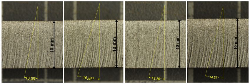
mental samples in Figures 1 and 2. These selected metal samples are ones from the series of
Materials 2021, 14, x FOR PEER REVIEW 12 of 17
three cuts performed under identical conditions. Respective values measured for all three
samples of selected metals are summarized in Table 6.
Figure 1. Steels and the respective average angles—the order from the left to the right right (WRN
(WRN norm):
norm): high strength steel
(1.7131), tool steel (1.2436), stainless steel (1.4541), Hardox 500 (trademark of the SSAB).
(1.7131), tool steel (1.2436), stainless steel (1.4541), Hardox 500 (trademark of the SSAB).Materials 2021, 14, 4032 11 of 16
Figure 1. Steels and the respective average angles—the order from the left to the right (WRN norm): high strength steel
(1.7131), tool steel (1.2436), stainless steel (1.4541), Hardox 500 (trademark of the SSAB).
Figure 2. Non-ferrous metals and the respective average angles—the order from the left to the right (WRN norm): copper
(2.0060), brass
(2.0060), brass (2.0402),
(2.0402), duralumin
duralumin (3.1325).
(3.1325).
Table 6. The declination angles measured for experimental samples in degrees (10 measurements for each case).
Table 6. The declination angles measured for experimental samples in degrees (10 measurements for each case).
Experiment Experiment Experiment Average Absolute Relative
Material
Material
Experiment Experiment Experiment Average Absolute Relative
I. I. II. II. III. III. Value
Value Uncertainty
Uncertainty Uncertainty
Uncertainty
High strength steel 10.62 10.97 10.06 10.55 ±0.37 3.6%
High strength steel 10.62 10.97 10.06 10.55 ±0.37 3.6%
Tool
Tool steel
steel 16.8616.86 16.2016.20 17.5317.53 16.86
16.86 ±0.54
±0.54 3.2%
3.2%
Stainless
Stainless steel
steel 12.2512.25 12.1212.12 12.7112.71 12.36
12.36 ±0.25
±0.25 2.0%
2.0%
Hardox
Hardox 500500 14.2214.22 14.3214.32 14.5914.59 14.37
14.37 ±0.15
±0.15 1.1%
1.1%
Copper 13.32 13.60 13.18 13.37 ±0.17 1.3%
Copper 13.32 13.60 13.18 13.37 ±0.17 1.3%
Brass 13.21 13.22 13.16 13.20 ±0.03 0.2%
Brass
Duralumin 13.4613.21 13.6013.22 13.5613.16 13.20
13.58 ±0.03
±0.11 0.2%
0.8%
Duralumin 13.46 13.60 13.56 13.58 ±0.11 0.8%
It can be seen that both the relative difference between the theoretical and the ex-
It can be seen that both the relative difference between the theoretical and the ex-
perimental values is below 5% (Table 5) and the relative uncertainty of measurement on
perimental values is below 5% (Table 5) and the relative uncertainty of measurement on
respective samples is also below 5% (Table 6). Therefore, the agreement of the theoretical
respective samples is also below 5% (Table 6). Therefore, the agreement of the theoretical
and the respective experimental results can be considered as very good.
and the respective experimental results can be considered as very good.
The presented model of the material cutting by AWJ is highly applicable on homo-
The presented model of the material cutting by AWJ is highly applicable on homo-
geneous and quasi-homogeneous materials—metals, rocks, concretes (if not reinforced or
geneous and quasi-homogeneous materials—metals, rocks, concretes (if not reinforced or
containing materials with extremely different mechanical properties), ceramics, glass and
containing materials with extremely different mechanical properties), ceramics, glass and
homogeneous plastics. The model needs additional “modification” for reinforced, sand-
homogeneous
wich, honeycomb plastics.
or otherThe model needs structures;
non-homogeneous additionalit “modification” for reinforced,
is applicable for these structures
when they are well described and both the position and influence of the inhomogeneity is
very predictable. The appropriate changes of the jet size when moving from one material
to another need to be calculated and the respective power loss needs to be evaluated and
taken into account.
The presented results indicate that use of the partial relations derived from the model
(theory) can be very effective in prediction of either the results of machining with certain
settings or calculation of the appropriate settings for achieving the required machining
results. Therefore, these partial equations, which can be derived from the basic theoretical
description and the respective model, can be used for preparation of control software with
very high precision.
7. Conclusions
The presented theoretical model includes almost all parameters of either the plain
water jet or the abrasive water jet, the machined material and other factors influencing
the quantity and the quality of the workpiece. The resulting equations yield many oppor-Materials 2021, 14, 4032 12 of 16
tunities to use only the partial relations among few parameters or factors for a transfer
of proven knowledge to the changed conditions. Some of these examples are presented
and the difference between the respective theoretical and experimental values is below
5%. Partial relations can be used in practice for preparation of control programs that can
calculate very exact settings of changeable parameters from the proven results obtained
with other settings or some “default settings”.
Funding: Experiments presented in this paper were partially supported by projects SP 2017/44, SP
2018/43, SP2019/26, SP2020/45 and SP2021/64 funded by the Ministry of Education, Youth and
Sports of the Czech Republic.
Institutional Review Board Statement: Not applicable.
Informed Consent Statement: Not applicable.
Data Availability Statement: Data sharing is not applicable to this article.
Conflicts of Interest: The author declares no conflict of interest.
Nomenclature
Coefficient of the velocity loss of the pure liquid jet in the interaction with material in a
α
solid state (energetic coefficient) . . . (–)
Experimentally determined coefficient of the abrasive water jet velocity loss in the
αe
interaction with material . . . (–)
Coefficient of the velocity loss of the pure liquid jet in the interaction with material in a
αn
solid state after the n-th pass of the jet through the same trace . . . (–)
γ Compressibility of the liquid for pressure po . . . (Pa−1 )
γo , γ p Shortened expression (1 − γpo ) . . . (–)
η Dynamic viscosity of the liquid . . . (N·s·m−2 )
Tilting angle of the cutting head measured in the plane containing the vector of the
θ traverse speed and stating the deviation of the jet axis and the perpendicular in the point
where the jet axis penetrates the inlet surface of material . . . (rad or ◦ )
Declination angle measured in the plane containing the vector of the traverse speed
ϑ and stating the deviation of the tangent to the striation at the outlet surface of material
and the inlet jet axis . . . (rad or ◦ )
Inclination angle measured in the plane perpendicular to the plane containing the vector
ϕ of the traverse speed and stating the deviation of the tangent to the side wall of the cut
and the inlet jet axis . . . (rad or ◦ )
Coefficient of the reflected liquid jet expansion due to the mixing with the disintegrated
χ
material (coefficient of the jet trace widening) . . . (–)
µ, µo Nozzle discharge coefficient . . . (–)
ρ, ρo Density of the liquid under the normal conditions . . . (kg·m−3 )
ρa Density of the abrasive material . . . (kg·m−3 )
ρj Density of the abrasive jet (conversion to homogeneous liquid) . . . (kg·m−3 )
ρm Density of material being machined . . . (kg·m−3 )
ρM Specific volume density of disintegrated material (including pores) . . . (kg·m−3 )
ρ∗M Specific mass density of the disintegrated material (excluding pores) . . . (kg·m−3 )
σ Strength of the target material (compressive, tensile or shear) . . . (Pa)
σm Strength of material being machined . . . (Pa)
σs Shear strength of the target material . . . (Pa)
Attenuation coefficient of the liquid jet between the nozzle outlet and the material
ξ
surface . . . (m−1 )
ξ∗ Attenuation coefficient of the liquid jet in the already formed kerf . . . (m−1 )
Attenuation coefficient of abrasive jet in the environment between the focusing tube outlet
ξj
and the material surface . . . (m−1 )
a Mean size of the element of material structure—the grain . . . (m)
an Mean size of abrasive particles formed in the mixing process . . . (m)
am Mean size of particles (elements) of material—grains or their chips . . . (m)Materials 2021, 14, 4032 13 of 16
ao Mean size of abrasive particles entering the mixing process . . . (m)
c Sound velocity inside the abrasive material . . . (m·s−1 )
Sound velocity inside the liquid used for preparation of the abrasive liquid jet (usually
co
water) . . . (m·s−1 )
Cf Friction coefficient of the liquid on the material element protruding to the jet flow . . . (–)
Coefficient modifying abrasive jet velocity in relation to the quantity of abrasive material
C1
input . . . (–)
Coefficient modifying abrasive jet velocity in relation to the ratio between the focusing
C2 tube diameter and the average abrasive particle size resulting from the mixing
process . . . (–)
Coefficient modifying abrasive jet velocity in relation to the friction inside the focusing
C3
tube . . . (–)
C4 Coefficient modifying abrasive jet velocity in relation to the focusing tube opening . . . (–)
Coefficient modifying abrasive water jet performance in relation to the changing content
CA of abrasive below the so-called saturation level (above this level the jet performance
increase is impossible and C A = 1) . . . (–)
Abrasive particle drag coefficient inside the liquid used for a preparation of the abrasive
CD
liquid jet (usually water) . . . (–)
do Water nozzle diameter (usually called orifice diameter) . . . (m)
da Focusing tube diameter . . . (m)
Resulting theoretical diameter of the outlet cylinder base of the sample cut by the abrasive
D water jet when the deformation caused by both the declination and the inclination angle is
calculated . . . (m)
Experimentally determined diameter of the cylindrical sample at the abrasive water jet inlet
Die
side . . . (m)
Experimentally determined diameter of the cylindrical sample at the abrasive water jet
Doe
outlet side . . . (m)
Diameter of the cylindrical sample at the abrasive water jet inlet side calculated from the
Dit
presented theoretical model . . . (m)
Diameter of the cylindrical sample at the abrasive water jet outlet side calculated from the
Dot
presented theoretical model . . . (m)
EP Specific surface energy of the abrasive material . . . (J)
f Friction coefficient of abrasive particle on the focusing tube wall . . . (–)
h Depth of material disintegration (depth of cut) . . . (m)
hlim Maximum depth of liquid jet penetration into material for the selected conditions . . . (m)
Depth of disintegration for the n-th pass of the jet through the same trajectory on the
hn
material surface . . . (m)
Summary depth of the jet penetration into material after the n-th pass of the jet trace in the
h∗n
case of multiple passes through the same trajectory on the material surface . . . (m)
H Material thickness . . . (m)
HV (Vickers’) material hardness . . . (N·m−2 )
k∗ “Dynamic” permeability of material . . . (m2 )
K Material hardness . . . (N·m−2 )
la Length of the focusing tube . . . (m)
Stand-off distance of the material surface or the investigated plane perpendicular to the
L
liquid jet axis from the nozzle or the focusing tube outlet . . . (m)
po Pressure of liquid before the nozzle (in the pump) . . . (Pa)
Pressure obtained from Bernoulli’s equation for a liquid with the density and the velocity of
pj
an abrasive jet . . . (Pa)
qa Abrasive mass flow rate . . . (kg·s−1 )
qw Water mass flow rate . . . (kg·s−1 )
Radius of the pre-set circle path of the jet axis intersection with surface of material plate
R
from which the sample is cut . . . (m)
Ratio between the quantity of non-damaged grains (i.e., not containing defects) and the total
SP
quantity of grains in the abrasive water jet . . . (–)
ti Interaction time . . . (s)
T Correction of the outlet edge of the sample caused by the taper angle . . . (m)
va Abrasive jet speed after the mixing process . . . (m·s−1 )Materials 2021, 14, 4032 14 of 16
vi Water jet speed before the mixing process . . . (m·s−1 )
vP Traverse speed of the jet trace on the material surface . . . (m·s−1 )
Traverse speed of the jet trace on the material surface modified by minimum traverse
veP
speed (v P + v Pmin ) . . . (m·s−1 )
Minimum traverse speed of cutting—correction for the zero traverse speed (the value
v Pmin should be equal to the average mean size of the abrasive particles after the mixing process
per minute, i.e., v Pmin = an /60) . . . (m·s−1 )
Limit traverse speed of the jet trace on the material surface calculated for the material
v Plim
thickness H . . . (m·s−1 )
Traverse speed of the jet trace on the material surface calculated for compensation of the
v Ptilt
deformation caused by the outlet declination angle 20◦ . . . (m·s−1 )
v PQ Traverse speed of the jet trace ensuring selected quality of cut walls . . . (m·s−1 )
References
1. Crow, S.C. A Theory of Hydraulic Rock Cutting. Int. J. Rock Mech. Min. 1973, 10, 567–584. [CrossRef]
2. Rehbinder, G. A Theory about Cutting Rock with Water Jet. Rock Mech. 1980, 12, 247–257. [CrossRef]
3. Hashish, M. A modeling study of metal-cutting with abrasive waterjets. J. Eng. Mater. Technol. 1984, 106, 88–100. [CrossRef]
4. Hashish, M. A model for abrasive—Waterjet (AWJ) machining. J. Eng. Mater. Technol. 1989, 111, 154–162. [CrossRef]
5. Hlaváč, L. Physical description of high energy liquid jet interaction with material. In Proceedings of the International Con-
ference Geomechanics, Hradec/Ostrava, Czechoslovakia, 24–26 September 1991; Rakowski, Z., Ed.; Balkema: Rotterdam,
The Netherlands, 1992; pp. 341–346.
6. Zeng, J.; Kim, T.J. An erosion model of polycrystalline ceramics in abrasive waterjet cutting. Wear 1996, 193, 207–217. [CrossRef]
7. Kovacevic, R.; Yong, Z. Modelling of 3D abrasive waterjet machining: Part 1—Theoretical basis. In Proceedings of the 13th
International Conference on Jetting Technology, Cagliari, Sardinia, Italy, 29–31 October 1996; Gee, C., Ed.; Mechanical Engineering
Publishing Ltd.: Bury St Edmunds, UK, 1996; pp. 73–82.
8. Yong, Z.; Kovacevic, R. Modelling of 3D abrasive waterjet machining: Part 2—Simulation of machining. In Proceedings of
the 13th International Conference on Jetting Technology, Cagliari, Sardinia, Italy, 29–31 October 1996; Gee, C., Ed.; Mechanical
Engineering Publishing Ltd.: Bury St Edmunds, UK, 1996; pp. 83–89.
9. Hlaváč, L.M. JETCUT—Software for prediction of high—Energy waterjet efficiency. In Proceedings of the 14th International
Conference on Jetting Technology, Brugge, Belgium, 21–23 September 1998; Louis, H., Ed.; Professional Engineering Publishing Ltd.:
London, UK, 1998; pp. 25–37.
10. Paul, S.; Hoogstrate, A.M.; van Luttervelt, C.A.; Kals, H.J.J. Analytical and Experimental Modeling of Abrasive Water Jet Cutting
of Ductile Materials. J. Mater. Process. Technol. 1998, 73, 189–199. [CrossRef]
11. Paul, S.; Hoogstrate, A.M.; van Luttervelt, C.A.; Kals, H.J.J. Analytical Modeling of the Total Depth of Cut in Abrasive Water Jet
Machining of Polycrystalline Brittle Materials. J. Mater. Process. Technol. 1998, 73, 206–212. [CrossRef]
12. Deam, R.T.; Lemma, E.; Ahmed, D.H. Modelling of the abrasive water jet cutting process. Wear 2004, 257, 877–891. [CrossRef]
13. Ma, C.; Deam, R.T. A correlation for predicting the kerf profile from abrasive water jet cutting. Exp. Therm. Fluid Sci. 2006, 30,
337–343. [CrossRef]
14. Hlaváč, L.M. Investigation of the abrasive water jet trajectory curvature inside the kerf. J. Mater. Process. Technol. 2009, 209,
4154–4161. [CrossRef]
15. Chen, F.L.; Wang, J.; Lemma, E.; Siores, E. Striation formation mechanisms on the jet cutting surface. J. Mater. Process. Technol.
2003, 141, 213–218. [CrossRef]
16. Orbanic, H.; Junkar, M. Analysis of striation formation mechanism in abrasive water jet cutting. Wear 2008, 265, 821–830.
[CrossRef]
17. Zhang, S.J.; Wu, Y.Q.; Wang, S. An exploration of an abrasive water jet cutting front profile. Int. J. Adv. Manuf. Technol. 2015, 80,
1685–1688. [CrossRef]
18. Shanmugam, D.K.; Wang, J.; Liu, H. Minimisation of kerf tapers in abrasive waterjet machining of alumina ceramics using a
compensation technique. Int. J. Mach. Tools Manuf. 2008, 48, 1527–1534. [CrossRef]
19. Hlaváč, L.M.; Hlaváčová, I.M.; Geryk, V.; Plančár, Š. Investigation of the taper of kerfs cut in steels by AWJ. Int. J. Adv. Manuf.
Technol. 2015, 77, 1811–1818. [CrossRef]
20. Wu, Y.Q.; Zhang, S.J.; Wang, S.; Yang, F.L.; Tao, H. Method of obtaining accurate jet lag information in abrasive water-jet
machining process. Int. J. Adv. Manuf. Technol. 2015, 76, 1827–1835. [CrossRef]
21. Srinivasu, D.S.; Axinte, D.A.; Shipway, P.H.; Folkes, J. Influence of kinematic operating parameters on kerf geometry in abrasive
waterjet machining of silicon carbide ceramics. Int. J. Mach. Tools Manuf. 2009, 49, 1077–1088. [CrossRef]
22. Alberdi, A.; Rivero, A.; de Lacalle, L.N.L.; Etxeberria, I.; Suarez, A. Effect of process parameter on the kerf geometry in abrasive
water jet milling. Int. J. Adv. Manuf. Technol. 2010, 51, 467–480. [CrossRef]
23. Hashish, M. Precision cutting of thick materials with AWJ. In Proceedings of the 17th International Conference on Water Jetting,
Mainz, Germany, 7–9 September 2004; Gee, C., Ed.; BHR Group: Cranfield, UK, 2004; pp. 33–45.
24. Hashish, M. AWJ Milling of Gamma Titanium Aluminide. J. Manuf. Sci. Eng. 2010, 132, 041005. [CrossRef]Materials 2021, 14, 4032 15 of 16
25. Boud, F.; Carpenter, C.; Folkes, J.; Shipway, P.H. Abrasive water jet cutting of a titanium alloy: The influence of abrasive
morphology and mechanical properties on workpiece grit embedment and cut quality. J. Mater. Process. Technol. 2010, 210,
2197–2205. [CrossRef]
26. Matsumura, T.; Muramatsu, T.; Fueki, S.; Hoshi, T. Abrasive water jet machining of glass with stagnation effect. CIRP Ann. 2011,
60, 355–358. [CrossRef]
27. Srinivas, S.; Babu, N.R. Penetration ability of abrasive waterjets in cutting of aluminum–silicon carbide particulate metal matrix
composites. Mach. Sci. Technol. 2012, 16, 337–354. [CrossRef]
28. Akkurt, A. Cut Front Geometry Characterization in Cutting Applications of Brass with Abrasive Water Jet. J. Mater. Eng. Perform.
2010, 19, 599–606. [CrossRef]
29. Chen, M.; Zhang, S.; Zeng, J.; Chen, B.; Xue, J.; Ji, L. Correcting shape error on external corners caused by the jet cut-in/cut-out
process in abrasive water jet cutting. Int. J. Adv. Manuf. Technol. 2019, 103, 849–859. [CrossRef]
30. Schwartzentruber, J.; Spelt, J.K.; Papini, M. Prediction of surface roughness in abrasive waterjet trimming of fiber reinforced
polymer composites. Int. J. Mach. Tools Manuf. 2017, 122, 1–17. [CrossRef]
31. Pahuja, R.; Ramulu, M.; Hashish, M. Surface quality and kerf width prediction in abrasive water jet machining of metal-composite
stacks. Compos. Part B Eng. 2019, 175, 107134. [CrossRef]
32. Anwar, S.; Axinte, D.A.; Becker, A.A. Finite element modelling of overlapping abrasive water jet milled footprints. Wear 2013,
303, 426–436. [CrossRef]
33. Wang, R.J.; Wang, C.Y.; Zheng, L.J.; Song, Y.X. Numerical simulation on the jet characteristics of abrasive jet. In Advances in
Materials Manufacturing Science and Technology XV, Special Edition Materials Science Forum; Zhu, R., He, N., Fu, Y., Yang, C.Y., Eds.;
Trans Tech Publications Ltd.: Zurich-Uetikon, Switzerland, 2014; Volume 770, pp. 257–262.
34. Wang, J.M.; Gao, N.; Gong, W.J. Abrasive waterjet machining simulation by SPH method. Int. J. Adv. Manuf. Technol. 2010, 50,
227–234.
35. Deepak, D.; Anjaiah, D.; Karanth, K.V.; Sharma, N.Y. CFD Simulation of Flow in an Abrasive Water Suspension Jet: The Effect of
Inlet Operating Pressure and Volume Fraction on Skin Friction and Exit Kinetic Energy. Adv. Mech. Eng. 2012, 186430. [CrossRef]
36. Hlaváč, L.M.; Hlaváčová, I.M.; Jandačka, P.; Zegzulka, J.; Viliamsová, J.; Vašek, J.; Mádr, V. Comminution of material particles by
water jets—influence of the inner shape of the mixing chamber. Int. J. Miner. Process. 2010, 95, 25–29. [CrossRef]
37. Hlaváčová, I.M.; Geryk, V. Abrasives for water-jet cutting of high-strength and thick hard materials. Int. J. Adv. Manuf. Technol.
2017, 90, 1217–1224. [CrossRef]
38. Aydin, G. Recycling of abrasives in abrasive water jet cutting with different types of granite. Arab. J. Geosci. 2014, 7, 4425–4435.
[CrossRef]
39. Aydin, G. Performance of recycling abrasives in rock cutting by abrasive water jet. J. Cent. South. Univ. 2015, 22, 1055–1061.
[CrossRef]
40. Jerman, M.; Orbanic, H.; Junkar, M.; Lebar, A. Thermal aspects of ice abrasive water jet technology. Adv. Mech. Eng. 2015,
1687814015597619. [CrossRef]
41. Borkowski, P.J. Application of abrasive-water jet technology for material sculpturing. Trans. Can. Soc. Mech. Eng. 2010, 34,
389–400. [CrossRef]
42. Schwartzentruber, J.; Papini, M. Abrasive water jet micro-piercing of borosilicate glass. J. Mater. Process. Technol. 2015, 219,
143–154. [CrossRef]
43. Haghbin, N.; Spelt, J.K.; Papini, M. Abrasive water jet micro-machining of channels in metals: Model to predict high aspect-ratio
channel profiles for submerged and unsubmerged machining. J. Mater. Process. Technol. 2015, 222, 399–409. [CrossRef]
44. Babu, M.N.; Muthukrishnan, N. Investigation of multiple process parameters in abrasive water jet machining of tiles. J. Chin. Inst.
Eng. 2015, 38, 692–700. [CrossRef]
45. Kvietkova, M.; Barcik, S.; Bomba, J.; Alac, P. Impact of chosen parameters on surface undulation during the cutting of agglomerated
materials with an abrasive water jet. Drewno 2014, 57, 111–123.
46. Servátka, M.; Fabian, S. Experimental research and analysis of selected technological parameters on the roughness of steel area
surface HARDOX 500 with thickness 40 mm cut by AWJ technology. Appl. Mech. Mater. 2013, 308, 13–18. [CrossRef]
47. Caydas, U.; Hascalik, A. A study on surface roughness in abrasive waterjet machining process using artificial neural networks
and regression analysis method. J. Mater. Process. Technol. 2008, 202, 574–582. [CrossRef]
48. Singh, R.; Singh, V.; Gupta, T.V.K. An experimental study on surface roughness in slicing tungsten carbide with abrasive water jet
machining. In Proceedings of the International Conference on Advances in Mechanical Engineering, ICAME 2020, Nagpur, India,
10–11 January 2020; Kalamkar, V.R., Monkova, K., Eds.; Springer: Singapore, 2021; pp. 353–359.
49. Jankovic, P.; Radovanovic, M.; Baralic, J.; Nedic, B. Prediction model of surface roughness in abrasive water jet cutting of
aluminium alloy. J. Balk. Tribol. Assoc. 2013, 19, 585–595.
50. Hreha, P.; Radvanska, A.; Knapcikova, L.; Królczyk, G.M.; Legutko, S.; Królczyk, J.B.; Hloch, S.; Monka, P. Roughness parameters
calculation by means of on-line vibration monitoring emerging from AWJ interaction with material. Metrol. Meas. Syst. 2015, 22,
315–326. [CrossRef]
51. Hlaváčová, I.M.; Mulicka, I. High-energy liquid jet technology—Risk assessment in practice. Int. J. Occup. Med. Env. 2012, 25,
365–374. [CrossRef] [PubMed]Materials 2021, 14, 4032 16 of 16
52. Fabian, S.; Salokyová, Š. AWJ cutting: The technological head vibrations with different abrasive mass flow rates. Appl. Mech.
Mater. 2013, 308, 1–6. [CrossRef]
53. Narayanan, C.; Balz, R.; Weiss, D.A.; Heiniger, K.C. Modelling of abrasive particle energy in water jet machining. J. Mater. Process.
Technol. 2013, 213, 2201–2210. [CrossRef]
54. Strnadel, B.; Hlaváč, L.M.; Gembalová, L. Effect of steel structure on the declination angle in AWJ cutting. Int. J. Mach. Tools
Manuf. 2013, 64, 12–19. [CrossRef]
55. Hlaváč, L.M.; Strnadel, B.; Kaličinský, J.; Gembalová, L. The model of product distortion in AWJ cutting. Int. J. Adv. Manuf.
Technol. 2012, 62, 157–166. [CrossRef]
56. Ahmed, D.H.; Naser, J.; Deam, R.T. Particles impact characteristics on cutting surface during the abrasive water jet machining:
Numerical study. J. Mater. Process. Technol. 2016, 232, 116–130. [CrossRef]
57. Lari, M.R.S.; Papini, M. Inverse methods to gradient etch three-dimensional features with prescribed topographies using abrasive
jet micro-machining: Part I—Modeling. Precis. Eng. 2016, 45, 272–284. [CrossRef]
58. Hlaváč, L.M. Application of water jet description on the de-scaling process. Int. J. Adv. Manuf. Technol. 2015, 80, 721–735.
[CrossRef]
59. Hlaváč, L.M.; Hlaváčová, I.M.; Vašek, J.; Jandačka, P.; Zegzulka, J.; Viliamsová, J.; Mádr, V.; Uhlář, R. Investigation Of Samples
From the High-Velocity Water Jet Driven Micro/Nano Particle Collider. Am. Soc. Mech. Eng. Press. Vessel. Pip. Div. 2010, 5,
119–126.
60. Galecki, G.; Sen, S.; Akar, G.; Li, Y.Q. Parametric Evaluation of Coal Comminution by Waterjets. Int. J. Coal Prep. Util. 2013, 33,
36–46. [CrossRef]
61. Hashish, M. Experimental studies of cutting with abrasive waterjets. In Proceedings of the 2nd U.S. Water Jet Conference, Rolla,
Missouri, 24–26 May 1983; Summers, D.A., Haston, F.F., Eds.; WJTA: St. Louis, MO, USA, 1983; pp. 379–389.
62. Hlaváč, L.M.; Krajcarz, D.; Hlaváčová, I.M.; Spadło, S. Precision comparison of analytical and statistical-regression models for
AWJ cutting. Precis. Eng. 2017, 50, 148–159. [CrossRef]
63. Hlaváč, L.M.; Hlaváčová, I.M.; Arleo, F.; Viganò, F.; Annoni, M.P.G.; Geryk, V. Shape distortion reduction method for abrasive
water jet (AWJ) cutting. Precis. Eng. 2018, 53, 194–202. [CrossRef]
64. Hlaváč, L.M.; Hlaváčová, I.M.; Plančár, Š.; Krenický, T.; Geryk, V. Deformation of products cut on AWJ x-y tables and its suppres-
sion. In Proceedings of the International Conference on Mechanical Engineering and Applied Composite Materials, MEACM
2017, Hong Kong, China, 23–24 November 2017; IOP Conference Series: Materials Science and Engineering; IOP Publishing:
Beijing, China, 2018; Volume 307, p. 0120152017.
65. Hlaváč, L.M.; Hlaváčová, I.M.; Vašek, J. Milling of materials by water jets—Acting of liquid jet in the cutting head. In TRANSACTIONS
of the VSB—Technical University of Ostrava; Engineering Series; VSB–Technical University of Ostrava: Ostrava, Czech Republic, 2007;
Volume LIII, pp. 73–84.You can also read