Simulation of Seawater Intrusion Area Using Feedforward Neural Network in Longkou, China - MDPI
←
→
Page content transcription
If your browser does not render page correctly, please read the page content below
water
Article
Simulation of Seawater Intrusion Area Using
Feedforward Neural Network in Longkou, China
Daiyuan Li 1,2,3 , Yongxiang Wu 1,2, *, Erkun Gao 2 , Gaoxu Wang 1,2 , Yi Xu 1,2 ,
Huaping Zhong 1,2 and Wei Wu 1,2
 1   State Key Laboratory of Hydrology-Water Resources and Hydraulic Engineering, Nanjing 210029, China;
     dyli@nhri.cn (D.L.); gxwang@nhri.cn (G.W.); xuyi@nhri.cn (Y.X.); hpzhong@nhri.cn (H.Z.);
     wwu@nhri.cn (W.W.)
 2   Hydrology and Water Resources Department, Nanjing Hydraulic Research Institute, Nanjing 210029, China;
     erkgao@mwr.gov.cn
 3   College of Hydrology and Water Resource, Hohai University, Nanjing 210098, China
 *   Correspondence: yxwu@nhri.cn

 Received: 7 June 2020; Accepted: 20 July 2020; Published: 24 July 2020

 Abstract: Reliable simulation of seawater intrusion (SI) is necessary for sustainable groundwater
 utilization. As a powerful tool, feedforward neural network (FNN) was applied to study seawater
 intrusion area (SIA) fluctuations in Longkou, China. In the present study, changes of groundwater
 level (GWL) were modeled by FNN Model 1. Then, FNN Model 2 was developed for fitting the
 relationship between GWL and SIA. Finally, two models were integrated to simulate SIA changes
 in response to climatic and artificial factors. The sensitivity analysis of each impact factor was
 conducted by the “stepwise” method to quantify the relative importance for SIA and GWL. The results
 from the integrated model indicated that this method could accurately reproduce SIA fluctuations
 when the Nash–Sutcliffe efficiency coefficient was 0.964, the root mean square error was 1.052 km2 ,
 the correlation coefficient was 0.983, and the mean absolute error was 0.782 km2 . The results of
 sensitivity analysis prove that precipitation and groundwater pumping for agriculture mainly affect
 fluctuations of SIA in the study area. It can be concluded that FNN is effectively used for modeling SI
 fluctuations together with GWL, which can provide enough support for the sustainable management
 of groundwater resources with consideration of crucial impact factors of seawater intrusion (SI).

 Keywords: seawater intrusion area; simulation; feedforward neural network; sensitivity analysis

1. Introduction
     Groundwater is easily accessible freshwater and an essential resource for domestic, agricultural,
and industrial purposes in coastal regions. With the rapid growth of human settlements and social
economy, these water demands increase the pressure on aquifer, and overexploitation of groundwater
resources has become an unavoidable problem in many coastal regions [1,2]. The excessive and
unregular exploitation from the coastal aquifer, hydraulically connected with sea, may cause seawater
intrusion (SI) [1,3], which seriously threatens the sustainability of groundwater utilization and
ecosystems. SI in different areas of the world has been reported in many researches and has obviously
become a global issue [2,4–7].
     In China, SI was founded as early as the 1960s, and the area was more than 2000 km2 in 2003 [8].
Longkou, like most coastal areas, has been continuously threatened by SI due to the overexploitation of
groundwater resources in the past five decades [8,9]. However, only a handful of previous studies paid
attention to it. Wu et al. built a three-dimensional seawater intrusion observation network to provide
insight on the characteristics of SI [10]. Xue et al. presented a three-dimensional miscible transport

Water 2020, 12, 2107; doi:10.3390/w12082107                                     www.mdpi.com/journal/water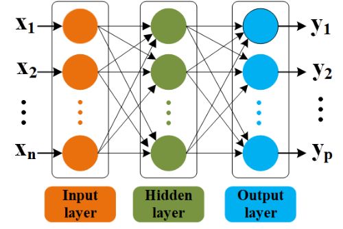
Water 2020, 12, 2107 2 of 17
model considering many important factors, such as variable density on fluid flow, precipitation
infiltration, and great discharge pumping wells [11]. Miao et al. built a three-dimensional (3D)
variable-density mathematical SI model using SEAWAT and proposed a Kriging surrogate model [12].
As we all know, the SI simulation is necessary for water managers to optimize groundwater utilization
and make effective strategies for recovery and prevention of SI. This paper tries to simulate SI
changes and identify controlling factors in Longkou by a simulation model, which will be helpful for
SI management.
SI, as well as groundwater level (GWL), is generally affected by natural and anthropogenic
factors, such as precipitation, surface water level, groundwater pumping, and artificial recharge [13].
Most of the previous researches focused on chloride concentration changes, which are an important
indicator to directly represent SI process [2,11,12]. However, the chloride concentrations at some points
are not stable and often have the extreme value from monitoring or simulation, which can increase
the uncertainty in SI management. To accurately predict SI developing trends, there is a need for
monitor station networks with wide distribution and high density. Besides, the chloride concentration
monitoring of groundwater is quite expensive. As an alternative, fluctuations of seawater intrusion
area (SIA) can be explored to represent SI process in this study, which might provide an easier and
more straightforward tool for coastal water management.
During the past several years, conceptual and physically based numerical models were successfully
applied to SI simulation in various conditions. Several numerical models such as SEAWAT [12,14–16],
FEFLOW [17,18], HYDROGEOSPHERE [19,20], and MOCDENS3D [21–23] have been widely used.
Although numerical models have a good performance in many cases, these methods require a large
amount of data and many parameters describing the groundwater system and physical properties for
the governing equation of groundwater flow and solute transport [24]. It is generally known that a
groundwater system is a highly complex and nonlinear system. Thus, a great quantity of data can cause
tremendous computational burden and an increase in model uncertainty [25]. Hence, the adaptability
of numerical models is poor due to the lack of abundant hydrogeological information. Fortunately,
the artificial neural network (ANN) is a strong tool for dealing with the complicated and uncertain
system, which demands only time series data for input variables without fully understanding physical
or hydrogeological properties [24,26,27].
Although ANN has some drawbacks such as overfitting and risk of using unrelated data,
the features including simplicity of use and high-speed run with acceptable accuracy have led many
researchers to apply it [28–35]. ANNs can be also developed as surrogate models to approximate
complex numerical variable density models [14,26,36–39]. This study focused on the application of
the feedforward neural network (FNN) in SIA simulation, which is a typical and frequently used
ANN structure. FNN has been widely and successfully used in the hydrological field, such as in the
estimation and prediction of streamflow [40–42], water quality [43], and groundwater level [44–46].
The objectives of the study are to evaluate the feasibility of the FNN in SIA simulation and to
identify which factors are crucial for SI management. In this paper, FNN models were developed to
simulate SIA changes together with GWL in a shallow coastal aquifer. The sensitivity analysis of each
impact factor was conducted by the “stepwise” method to quantify the relative importance for SIA
and GWL.
2. Materials and Methods
2.1. Study Area and Data
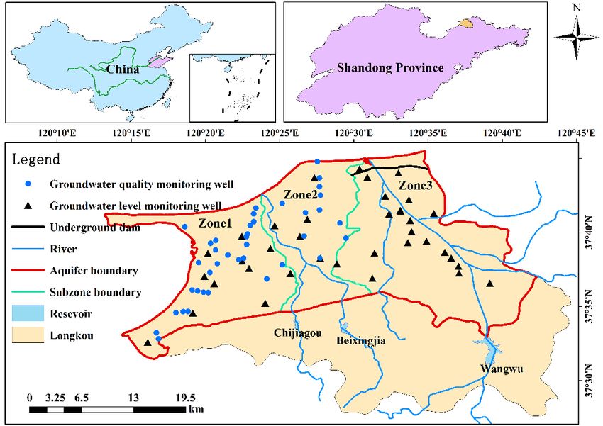
The study area is located at Longkou, Shandong Province, China, which lies between 120◦ 130 14”
to 120◦ 440 46” east longitude and 37◦ 270 30” to 37◦ 470 24” north latitude (Figure 1). The Longkou is a
county-level administrative region, whose population is about 718,000. As shown in Figure 1c, there are
three key reservoirs, named Wangwu, Chijiagou, and Beixingjia. The red frame area in Figure 1c shows
that the main groundwater aquifer, composed of layer Quaternary loose sediment, is situated at the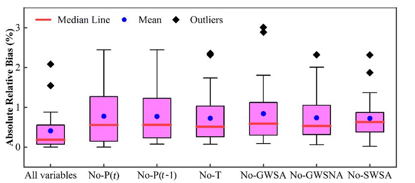
Water 2020, 12, 2107                                                                                                   3 of 17

northern plain of Longkou in terms of the results of the hydrogeological investigation. The study area
is approximately 600 km2 , which is approximately 67% of the Longkou, and the total length of the
coastline is 68.38 km. As a semihumid monsoon continental climate area, the annual average rainfall
is around 594.1 mm (years 1955–2017), out of that 73% occurs from June to September. The annual
mean temperature is around 11.8 ◦ C, and the maximum and minimum temperatures are 38.3 ◦ C and
−21.3 ◦ C, respectively.
              Water 2020, 12, x FOR PEER REVIEW                                       4 of 18

                                                        (a)                              (b)

                                                                                               (c)

      Figure 1. (a) Figure
                    Location1. (a) Location of Shandong Province in China; (b) location of Longkou in Shandong Province;
                                   of Shandong Province in China; (b) location of Longkou in Shandong Province;
                    (c) description of the study area.
      (c) description of the study area.

     In 1979, SI was first found in the Longkou. From the 1980s to the early 21st century, the amount of
groundwater exploitation has been steadily increased in order to cope with the substantial growth
of water resource demand. Gradually, SI developed from patches to strips, which posed a severe
threat to sustainable development of the social economy and protection of the ecological environment.
In order to gain insight on the SI process, the Longkou government made an effort to monitor GWL
and groundwater quality, which provides much support to the present study. Figure 1c displays the
distributions of GWL-monitoring wells and groundwater quality-monitoring wells.
     In this study, six-monthly groundwater chloride concentration (years 2005–2017) and the data
(years 2000–2017), including monthly average GWL, monthly precipitation (P), and monthly average
                   Figure 2. Changes of monthly average groundwater level (GWL) in three zones (years 2000–2017).
temperature (T), were collected from the Longkou government. Besides, annual groundwater supply
for agriculture (GWSA), annual groundwater supply for nonagriculture (GWSNA), and annual surface
water supply for agriculture (SWSA) were obtained from the Longkou Water Resources Bulletin. It is
noted that GWSNA is composed of domestic and industrial water supply. Then, the datasets of
annual water supply for agriculture were processed into a monthly value based on crop structure,
water demand of crop growth period, and distribution of monthly precipitation. The monthly GWSNA
was calculated by the average distribution of annual value.
     In addition, according to the hydrogeological data and management demand, the study area was
divided into three zones of water resources management (Figure 1c), named Zone1, Zone2, and Zone3.
Figure 2 illustrates the changes of monthly average GWL in the three zones. It is apparent that GWL
changes of the three   zones are similar in trend, and there are high fluctuations. Based on the evaluation
                  Figure 3. Changes of six-monthly seawater intrusion area (SIA) in the study area (years 2005–2017).
results of the second national water resources investigation in Longkou, the annual average quantity
of total recharge is about 21.49 million cubic meters, 17.71 million cubic meters, and 58.15 million
cubic meters in Zone1, Zone2, and Zone3, respectively. Recharge sources of the unconfined aquifer are
similar in three zones, which mainly include the infiltration of precipitation, infiltration of agricultural
water, infiltration of rivers, and lateral inflow from the southern mountainous area. The proportions
of four recharge sources in annual average quantity of total recharge are approximately 43%, 42%,
5%, and 10% in Zone1; 43%, 37%, 8%, and 10% in Zone2; and 37%, 40%, 17%, and 6% in Zone3.
(c)
Water 2020, 12, 2107 4 of 17
Water 2020, 12, x FOR PEER REVIEW 4 of 18
The discharging sources in Zone1 and Zone2 (a) are primarily composed(b)of groundwater pumping,
evaporation, and natural outflow into the sea, in which the annual average quantity of groundwater
pumping is about 2.318 million cubic meters, 1.914 million cubic meters, and 5.232 million cubic meters,
respectively. However, it is different from Zone1 and Zone2 in that there is no natural outflow into
the sea in Zone3,Figure
because the underground dam was built 1.2 km from the estuary in 1994 (Figure 1),
(c) Province;
1. (a) Location of Shandong Province in China; (b) location of Longkou in Shandong
which completely blocks the
(c) description hydraulic
of the study area. connection between sea and groundwater system.
Figure 1. (a) Location of Shandong Province in China; (b) location of Longkou in Shandong Province;
(c) description of the study area.
Figure 2. Changes of monthly average groundwater level (GWL) in three zones (years 2000–2017).
Figure 2. Changes of monthly average groundwater level (GWL) in three zones (years 2000–2017).
The SIA, where the chloride concentration is more than 250 mg/L, was acquired by inverse distance
weight interpolation (IDW) of chloride concentration of monitoring wells. It is noted that the area
where the chloride concentration is more than 250 mg/L in Zone3 does not need to be considered
in the simulative model because of the underground dam. In other words, the GWL drawdown
can not make seawater move into land in Zone3. Hence, the SIA referred to the total area of Zone1
and Zone2, which was modeled in this study. As shown in Figure 3, SIA was relieved from 134.4
km2 in December 2007 to 115.3 km2 in June 2011, but it showed an increasing trend from 2013 to
2017. Therefore, accurate SIA simulation is very significant for the Longkou government to prevent SI
from exacerbating.Figure 2. Changes of monthly average groundwater level (GWL) in three zones (years 2000–2017).
Figure 3. Changes of six-monthly seawater intrusion area (SIA) in the study area (years 2005–2017).
Figure 3. Changes of six-monthly seawater intrusion area (SIA) in the study area (years 2005–2017).
Figure 3. Changes of six-monthly seawater intrusion area (SIA) in the study area (years 2005–2017).
2.2. Feedforward Neural Network
ANN is distributed parallel processors imitating the structure and operation of the human
brain [13]. It seems to be a “black” model or empirical model and has self-organization, self-learning,
and strong nonlinear ability. The FNN, which is a typical ANN architecture, has been widely applied
to kinds of hydrological research. A common FNN is composed of three separate layers, namely, input,
hidden, and output layers, each consisting of processing neurons, with interconnections occurring
between neurons in adjacent layers.
Figure 4 shows a typical three-layer FNN architecture. The number of neurons in input layers,
as well as in output layers, is determined by input variables and targets of the building model.
The number of hidden layers is chosen for the best simulation result. Each processing node is
interconnected across layers by special nonlinear transfer functions, which means the state of neurons
of each layer only has an impact on neurons of the next layers. The distinguishing feature of FNN
is the forward propagation of input signals and the backward propagation of the error. During thestrong nonlinear ability. The FNN, which is a typical ANN architecture, has been widely applied to
kinds of hydrological research. A common FNN is composed of three separate layers, namely, input,
hidden, and output layers, each consisting of processing neurons, with interconnections occurring
between neurons in adjacent layers.
Figure 4 shows a typical three-layer FNN architecture. The number of neurons in input layers,
Water 2020,
as 12,
well2107
as in output layers, is determined by input variables and targets of the building model. The 5 of 17
number of hidden layers is chosen for the best simulation result. Each processing node is
interconnected across layers by special nonlinear transfer functions, which means the state of neurons
trainingofstage, the only
each layer connection weights
has an impact and bias
on neurons arenext
of the adjusted
layers. repeatedly until afeature
The distinguishing minimum
of FNNacceptable
is
the forward
error between propagation
simulation and of input signals
observation and the backward
is achieved. propagation of
The mathematical the error. During
expression the is given
of output
training
by Equation stage, the connection weights and bias are adjusted repeatedly until a minimum acceptable
(1).
error between simulation and observation m
X is achieved.
n
X The mathematical expression of output is
given by Equation (1). y k = fo ( w jk × fh ( wij Xi + b j ) + bk ) (1)
j=1 m i=
n 1
yk = f o ( w jk × f h ( wij X i + b j ) + bk ) (1)
where i, j, and k refer to the ith input node,j =the 1 i =1
jth hidden node, and the kth output node, respectively.
n and mwhere
are the
i , number
j , and kofrefer
input nodes
to the i th and
inputhidden
node, thenodes. w andnode,
j th hidden b represent
and the the
k thweight and the bias.
output node,
fh and frespectively.
o are the activation functions of hidden layers and output layers. X and
n and m are the number of input nodes and hidden nodes. w and b represent the y represent the input
weight and
and output value. the bias. f h and f o are the activation functions of hidden layers and output layers. X
and y represent the input and output value.
Figure 4. Basic
Figure architecture
4. Basic architectureofoffeedforward neural
feedforward neural network
network withwith
threethree
layers.layers.
A variety of components
A variety of components need
need totobebeconsidered
considered ininorderorder to to build
build an appropriate
an appropriate FNN model,
FNN model,
includingincluding the selection
the selection of inputof input variables,
variables, the number
the number of hidden
of hidden layers
layers andand nodes,
nodes, thethetransfer
transferfunction
of hiddenfunction
layers of and
hidden layerslayers,
output and output layers,algorithm,
training training algorithm, and criteria
and criteria of model
of model performance.
performance.
The selection of input variables is one of the most important steps in the FNN development. It
The selection of input variables is one of the most important steps in the FNN development. It is
is noted that not all of the potential input variables will be equally informative because some may be
noted that not all ofnoisy,
uncorrelated, the potential
or have noinput variables
significant will be
relationship withequally informative
the output because
of models [47]. some may be
Commonly,
uncorrelated, noisy,
initial input or have
variables no significant
are decided based onrelationship
a priori knowledgewithabout
the output of models properties.
system fundamental [47]. Commonly,
Some variables
initial input researches are
employed
decideda cross-correlation
based on a priori method to revealabout
knowledge linearsystem
dependence between two
fundamental properties.
variable time series. Unfortunately, most of the relationship between
Some researches employed a cross-correlation method to reveal linear dependence between two two variables in the natural
groundwater system is nonlinear. In this study, a combination of the priori knowledge and
variable time series. Unfortunately, most of the relationship between two variables in the natural
correlation coefficient method was used for determining appropriate input variables.
groundwater system is nonlinear. In this study, a combination of the priori knowledge and correlation
The activation function is vital to the network, which makes neurons have the ability of
coefficient method
perception. was
The used forfunction
tan-sigmoid determining appropriate
was applied to hiddeninput variables.
layers and output layers and is described
Theasactivation
Equation (2).function is vital to the network, which makes neurons have the ability of perception.
The tan-sigmoid function was applied to hidden 2layers and output layers and is described as
f ( x) = (2)
Equation (2). (1 + e−2 x)− 1
2
f (x) = (2)
(1 + e−2x ) − 1
Levenberg–Marquardt algorithm (LM) was applied to train FNN models in the present study,
which is a widely popular training algorithm [18]. LM algorithm is a modification of the Newton
algorithm for finding an optimal solution about the minimization problem. It has great computational
and memory requirements [34], and is faster and less easily trapped in local minima than other
optimization algorithms.
In addition, one hidden layer FNN was used, and the number of hidden nodes was also determined
by a trial-and-error procedure.
The model performance was evaluated by statistical parameters involving Nash–Sutcliffe efficiency
coefficient (E), root mean squared error (RMSE), correlation coefficient (R), and mean absolute error
(MAE). The four statistical indicators are defined as follows:
n
(hot − hct )2
P
t=1
E = 1− n
(3)
P 2
(hot − hot )
t=1Water 2020, 12, 2107 6 of 17
v
n
t
1X
RMSE = (hot − hct )2 (4)
n
t=1
n
P
(hot − hot )(hct − hct )
t=1
R= s (5)
n
P 2 2
(hot − hot ) (hct − hct )
t=1
n
1X
MAE = |hot − hct | (6)
n
t=1
where hct and hot are simulated and observed values at time t, hct and hot are the average of simulated
and observed output series, respectively. The closer that RMSE and MAE are to 0, and E and R are to 1,
the better simulations match to observations.
2.3. Application for Seawater Intrusion Area Simulation
SI is caused by the comprehensive function of seawater system and coastal groundwater system.
Unregulated and excessive exploitation of groundwater is a primary factor in many coastal regions.
The GWL changes provide a direct measure of groundwater development, and SIA can display the
degree of SI. Besides, critical information about aquifer dynamics is often embedded in the continuously
recorded time series. In this paper, changes of SIA together with GWL were simulated based on
FNN, and Figure 5 depicts the model structure, in which n represents the number of input variables.
The steps of the model are as follows:
1. The FNN Model 1 is built to simulate GWL changes effected by climatic factors and
human activities.
2. The FNN Model 2 is developed to simulate the relationship between GWL of three zones
and SIA.
3. FNN Model 1 and FNN Model 2 are integrated, which means that the results of the FNN
Model 1 are viewed as the input data of the FNN Model 2. The integrated model can help managers
understand SIA changes in response to natural and artificial factors.
4. The sensitivity of each factor is studied by the “stepwise” method, in which input variables are
deleted one at a time and the corresponding model is developed and validated. Then, the relative
importance ranks are obtained by comparison of model performance criteria, and crucial impact factors
are identifiedWater
for2020,
SIA and GWL.
12, x FOR PEER REVIEW 7 of 18
Figure Figure 5. Configurationof
5. Configuration of the
the model
model for for
SIA SIA
simulation.
simulation.
3. Results and Discussion
3.1. Groundwater Level Simulation
3.1.1. Determination of FNN Model 1 Architecture
As aforementioned, the determination of model architecture should be learned from the
fundamental conceptual knowledge of the study area. According to the water budget description of
the aquifer in Section 2.1, the major influence factors include infiltration of precipitation, infiltration
of agricultural water, groundwater exploitation, and evaporation. It is noted that the influence of
lateral inflow and outflow into sea for the groundwater system was not considered because the
quantity is so small that they have a weak impact on GWL. The infiltration of rivers was likewise
ignored in the model due to the long drying-out of rivers. Besides, the evaporation of groundwater
system is extremely difficult to quantify over space and time. As an alternative, the monthly averageWater 2020, 12, 2107 7 of 17
3. Results and Discussion
3.1. Groundwater Level Simulation
3.1.1. Determination of FNN Model 1 Architecture
As aforementioned, the determination of model architecture should be learned from the
fundamental conceptual knowledge of the study area. According to the water budget description of
the aquifer in Section 2.1, the major influence factors include infiltration of precipitation, infiltration of
agricultural water, groundwater exploitation, and evaporation. It is noted that the influence of lateral
inflow and outflow into sea for the groundwater system was not considered because the quantity is
so small that they have a weak impact on GWL. The infiltration of rivers was likewise ignored in
the model due to the long drying-out of rivers. Besides, the evaporation of groundwater system is
extremely difficult to quantify over space and time. As an alternative, the monthly average temperature
was considered as an input variable in this model. In the study area, there is a combination of surface
water utilization from water storage projects and groundwater pumping for irrigation. When the total
amount of groundwater and surface water for irrigation is constant, the response of groundwater
system is obviously different. This is because GWSA is both a discharge and a recharge resource
and SWSA is only a recharge resource. According to whether it can feed the aquifer, groundwater
exploitation was divided into GWSA and GWSNA. Also, the initial monthly average GWL was
considered as a fundamental input.
It should be noted that different time lags of factors for model performance were considered.
Different lengths of precipitation, temperature, GWSA, GWSNA, and SWSA varying from 1 to 6
months were tested by the trial-and-error method. It was found that the delay contribution of factors,
except precipitation, had no positive effect on model performance, and one time-lag of precipitation
had an optimal performance. The autocorrelation coefficients for identifying appropriated lengths
of GWL time-lag of three zones from 1 to 6 months are given in Table 1. One time-lag was highly
significant with autocorrelation coefficients of 0.975, 0.990, and 0.981 in three zones, respectively.
Table 1. Autocorrelation coefficients of monthly average GWL in three zones.
Time-Lag Zone1 Zone2 Zone3
t−1 0.975 0.990 0.981
t−2 0.927 0.969 0.944
t−3 0.879 0.948 0.910
t−4 0.839 0.931 0.882
t−5 0.812 0.919 0.858
t−6 0.790 0.910 0.838
Note: t represents the monthly time step of feedforward neural network (FNN) Model 1.
In summary, input variables of FNN Model 1 included monthly precipitation at time t (P(t)),
monthly precipitation at time t − 1 (P(t − 1)), monthly average temperature at time t (T(t)),
monthly groundwater supply for agriculture at time t (GWSA(t)), monthly groundwater supply
for nonagriculture at time t (GWSNA(t)), monthly surface water supply for agriculture at time t
(SWSA(t)), monthly average GWL of Zone1 at time t − 1 (GWL1 (t − 1)), monthly average GWL of
Zone2 at time t − 1 (GWL2 (t − 1)), and monthly average GWL of Zone3 at time t − 1 (GWL3 (t − 1)).
It is noted that t represents the monthly time step of FNN Model 1.
Output variables of FNN Model 1 included monthly average GWL of Zone1 at time t (GWL1 (t)),
monthly average GWL of Zone2 at time t (GWL2 (t)), and monthly average GWL of Zone3 at time
t (GWL3 (t)). The datasets were separated into two different parts. For the training set, 80% of the
collected and preprocessed data were used, and 20% were used for the validation set. The activation
function of hidden layers and output layers, the number of hidden layers, and the training algorithm
in FNN Model 1 are described in Section 2.2. The number of nodes in the hidden layer was determinedWater 2020, 12, 2107 8 of 17
by the trial-and-error method. The trial-and-error procedure started with five hidden neurons initially,
and the number of hidden neurons was increased to twenty. The optimum number of hidden neurons
was found to be ten.
3.1.2. Results of FNN Model 1
Figure 6 depicts the monthly average GWL simulation of three zones for the validation stage
(July 2014–December 2017). It is noted that the blue line represents the observed GWL, and the red
line represents the simulated GWL in Figure 6a–c. These figures indicate that there was a good fitting
between observation and simulation in three zones. The performances of FNN Model 1 in terms of E,
RMSE, R, and MAE are presented in Table 2. It is apparent from this table that during the validation
period, E value varied from 0.908 to 0.997, RMSE value varied from 0.133 m to 0.251 m, R value varied
from 0.965 to 0.998, and MAE value varied from 0.100 m to 0.184 m. Hence, FNN Model 1 has the
ability to model GWL fluctuations with reasonable accuracy, which can help managers obtain more
information on the groundwater system to enhance groundwater resource management.
Water 2020, 12, x FOR PEER REVIEW 9 of 18
(a) (d)
(b) (e)
(c) (f)
Figure 6. Figure 6. Comparison
Comparison between observation
between observation andand
simulation of monthly
simulation of average
monthly GWL using FNN
average GWL using
Model 1: (a−c) Line plot of results in Zone1, Zone2, and Zone3 during validation period, respectively;
FNN Model 1: (a–c) Line plot of results in Zone1, Zone2, and Zone3 during validation period,
(e−f) Scatter plot of results in Zone1, Zone2, and Zone3 during training and validation period,
respectively; (d–f) Scatter plot of results in Zone1, Zone2, and Zone3 during training and validation
respectively.
period, respectively.
Table 2. Statistical indicators of FNN Model 1 performance during training and validation period.
Zone Period E RMSE (m) R MAE (m)
Training 0.994 0.169 0.997 0.127
Zone1
Validation 0.908 0.251 0.970 0.184
Training 0.996 0.133 0.998 0.100
Zone2
Validation 0.954 0.134 0.977 0.101
Training 0.997 0.133 0.998 0.104
Zone3
Validation 0.911 0.133 0.965 0.102Water 2020, 12, 2107 9 of 17
Table 2. Statistical indicators of FNN Model 1 performance during training and validation period.
Zone Period E RMSE (m) R MAE (m)
Training 0.994 0.169 0.997 0.127
Zone1
Validation 0.908 0.251 0.970 0.184
Training 0.996 0.133 0.998 0.100
Zone2
Validation 0.954 0.134 0.977 0.101
Training 0.997 0.133 0.998 0.104
Zone3
Validation 0.911 0.133 0.965 0.102
The names of abbreviations are described in Table A1.
3.2. Seawater Intrusion Area Simulation
3.2.1. Determination of FNN Model 2 Architecture
Seawater intrusion means that the balanced interface between groundwater system and seawater
system moves to land. In the study area, the correlation coefficient between six-monthly average sea
level and six-monthly SIA was about −0.179, which indicated that variations of sea level have a little
influence on SIA fluctuations during the simulated period (years 2005–2017). Therefore, this section
pays attention to the relationship between GWL and SIA. In FNN Model 2, the six-monthly average
GWL of three zones and initial SIA were considered in the input layer. Correlation coefficients between
GWL of each zone and SIA are presented in Table 3. Further, different lengths of GWL varying from 0
to 6 time steps were tested by the trial-and-error method. Altogether, it was found that time lag > 1 of
GWL in each zone does not provide a significant contribution to the model performance. In short,
input variables of FNN Model 2 included GWL1 (k), GWL1 (k − 1), GWL2 (k), GWL2 (k − 1), GWL3 (k),
and GWL3 (k − 1). It should be noted that k represents the six-monthly time step of FNN Model 2.
The output variable only included SIA at time k. In addition, datasets were divided into two different
parts—80% of the collected data were viewed as the training set; the other 20% for the validation set.
Table 3. The correlation coefficient between GWL of three zones and SIA, respectively.
Time-Lag Zone1 Zone2 Zone3
k 0.845 0.896 0.543
k−1 0.831 0.910 0.681
k−2 0.770 0.875 0.724
k−3 0.705 0.834 0.747
k−4 0.601 0.799 0.746
k−5 0.463 0.754 0.759
k−6 0.304 0.699 0.760
Note: k represents the six-monthly time step of FNN Model 2.
In FNN Model 2, the activation function of hidden layers and output layers, the number of hidden
layers, and the training algorithm are described in Section 2.2, as well as FNN Model 1. The number of
hidden neurons in the network was identified by various trials. The trial-and-error procedure started
with two hidden neurons initially, and the number of hidden neurons was increased to twenty. It was
found that thirteen neurons were optimal for model performance.
3.2.2. Results of FNN Model 2
Figure 7 presents the simulation of six-monthly SIA by FNN Model 2 for the training and validation
period (years 2005–2017). It illustrated that there was a good matching between observation and
simulation. The four statistical indicators of model performance are shown in Table 4. It can be
seen from the table that during the training, the statistical indicators E, RMSE, R, and MAE were
0.978, 0.877 km2 , 0.990, and 0.575 km2 , respectively, and the corresponding parameters were 0.821,
0.493 km2 , 0.941, and 0.295 km2 during the validation. The values of statistical indicators impliedWater 2020, 12, 2107 10 of 17
that the performance of FNN Model 2 was satisfactory during both the training and the validation
period. Overall, the FNN Model 2 is capable of an understanding relationship between SIA and GWL.
Water 2020, 12, x FOR PEER REVIEW 11 of 18
Meanwhile, the results prove that SIA and GWL are closely related, which is in agreement with the
previous research
Water 2020, [9].
12, x FOR PEER REVIEW 11 of 18
(a) (b)
Figure 7. Comparison between (a) observation and simulation of six-monthly SIA (b) using FNN Model 2:
(a)
Figureline
Figure plot of results;
7. Comparison
7. Comparison (b) scatter
between plot of
betweenobservation results.
observationand
and simulation
simulation of
of six-monthly
six-monthlySIA
SIAusing
usingFNN
FNNModel
Model2: 2: (a)
line (a)
plotline
ofplot of results;
results; (b) scatter
(b) scatter plot plot of results.
of results.
Table 4. Statistical indicators of FNN Model 2 during the training and validation period.
Table 4. Statistical
Table 4. Statisticalindicators
indicatorsof
of FNN Model22during
FNN Model duringthethe training
training andand validation
validation period.
period.
Period E RMSE (km2) R MAE (km2)
22
Period
Training E
Period
0.978 E RMSE
RMSE (km
0.877(km) ) R R
MAE
0.990 (km2 ) MAE 0.575
(km2)
Training
Validation 0.978
Training
0.821 0.978 0.877
0.877
0.493 0.990
0.990 0.9410.575 0.575
0.295
Validation 0.821
Validation 0.821 0.493
0.493 0.941 0.9410.295 0.295
3.2.3. Integrated Model The names of abbreviations are described in Table A1.
3.2.3. Integrated Model
In this section,
3.2.3. Integrated Model FNN Model 1 and FNN Model 2 are integrated, which can help managers study
In this section, FNN Model 1 and FNN Model 2 are integrated, which can help managers study
the SIA fluctuations in response to water exploitation activities and climate factors. The results of
the SIA section,
In this fluctuationsFNN in Model
response to water
FNNexploitation activities and climate factors. The results of study
monthly average GWL (years 12005–2017)
and ModelFNN
from 2 are integrated,
Model 1 werewhich can help
processed intomanagers
six-monthly
monthly
theaverage average
SIA fluctuations GWL
in (years
response 2005–2017)
to water from FNN
exploitation Model 1
activitieswere
and processed
climate into
factors.six-monthly
The results of
GWL, which was considered as input data for FNN Model 2. Figure 8 displays a comparison
average GWL, which was considered as input data for FNN Model 2. Figure 8 displays a comparison
monthly
between average
simulation and observation, and statistical indicators of model performance foraverage
GWL (years 2005–2017) from FNN Model 1 were processed into six-monthly the
between simulation and observation, and statistical indicators of model performance for the
GWL, which was
computation considered as input dataEfor FNNforModel 2.RMSE
Figure 8 displays a comparison between
period are shown, in which scored 0.964, scored for 1.052 km
computation period are shown, in which E scored for 0.964, RMSE scored for 1.052 km , R scored for for
2, R scored
2
simulation
0.983, and
0.983, and
and MAEobservation,
MAE scored
scoredforforand
0.782statistical
0.782 km indicators
km2.. Therefore,
2
Therefore, of model performance
theintegrated
the integrated modelhad
model had for
anan the computation
excellent
excellent period
performance
performance
arebased
shown, 2for
based on statistical indicators and graphs, which can be used for accurately predicting SI MAE
on in which
statistical E scored
indicators for 0.964,
and RMSE
graphs, scored
which for
can 1.052
be km
used , R scored
accuratelyfor 0.983, and
predicting SI
development.
scored 2
for 0.782 km . Therefore, the integrated model had an excellent performance based on statistical
development.
indicators and graphs, which can be used for accurately predicting SI development.
(a) (b)
Figure 8. Comparison between observation and simulation of six-monthly SIA using integrated
model: (a) line plot of results;
(a) (b) scatter plot of results. (b)
Figure
Figure
3.3. 8. 8.
Sensitivity Comparison
Comparison between
between
Analysis for GWL and observation
observation andand
SIA Simulation simulation
simulation of six-monthly
of six-monthly SIA SIA using
using integrated
integrated model:
model: (a) line plot of results; (b) scatter plot
(a) line plot of results; (b) scatter plot of results. of results.
After the FNN models for GWL and SIA simulation were developed, one of the significant
3.3. objectives
Sensitivity
3.3. Sensitivity inAnalysis
this study
Analysis forwas
for GWL
GWLto and
gain a better
and SIA
SIA understanding of natural and anthropogenic factors for
Simulation
Simulation
the coastal groundwater system. In other words, the relative importance of each factor for
After
Afterthe
fluctuationstheFNN
ofFNN
GWLmodels
models
and SIAfor GWL
forwasGWL and
and SIA
analyzed. SIA simulation
simulation
In this were
section, were
the developed,
developed,
“stepwise” one
one
method, of
ofinthethe significant
significant
which one
objectives
input variable was deleted and the corresponding model was developed and validated, is outlined,for
objectives in this
in study
this studywaswas to gain
to gaina better
a understanding
better understanding of natural
of naturaland
andanthropogenic
anthropogenic factors
factors forthe
theandcoastal groundwater
statistical indicators ofsystem. In other words,
model performance the relative
are compared. Basedimportance
on the inputofvariables
each factor
set of for
fluctuations of GWL and SIA was analyzed. In this section, the “stepwise” method, in which oneWater 2020, 12, 2107 11 of 17
coastal groundwater system. In other words, the relative importance of each factor for fluctuations
of GWL and SIA was analyzed. In this section, the “stepwise” method, in which one input variable
was deleted and the corresponding model was developed and validated, is outlined, and statistical
indicators of model performance are compared. Based on the input variables set of FNN Model 1 in
Section 3.1, six input scenarios for sensitivity analysis were established, which are presented in Table 5.
The absolute relative bias of simulation was displayed by a box plot to make a qualitative analysis.
The relative importance rank of each factor was obtained based on the ratio, which is described by
Equation (7). A ratio value >1 represents that the elimination of the factor reduces the simulative
accuracy. Hence, the larger the ratio, the stronger the influence of the missing factor on the target.
MAE without one f actor in input layer
ratio = (7)
MAE with all variables
Table 5. Six input scenarios sets for sensitivity analysis.
No. Scenarios Input Variables Set
- All variables P(t), P(t − 1), T(t), GWSA(t), GWSNA(t), SWSA(t), GWL1 (t − 1), GWL2 (t − 1), GWL3 (t − 1)
1 No-P(t) P(t − 1), T(t), GWSA(t), GWSNA(t), SWSA(t), GWL1 (t − 1), GWL2 (t − 1), GWL3 (t − 1)
2 No-P(t − 1) P(t), T(t), GWSA(t), GWSNA(t), SWSA(t), GWL1 (t − 1), GWL2 (t − 1), GWL3 (t − 1)
3 No-T P(t), P(t − 1), GWSA(t), GWSNA(t), SWSA(t), GWL1 (t − 1), GWL2 (t − 1), GWL3 (t − 1)
4 No-GWSA P(t), P(t − 1), T(t), GWSNA(t), SWSA(t), GWL1 (t − 1), GWL2 (t − 1), GWL3 (t − 1)
5 No-GWSNA P(t), P(t − 1), T(t), GWSA(t), SWSA(t), GWL1 (t − 1), GWL2 (t − 1), GWL3 (t − 1)
6 No-SWSA P(t), P(t − 1), T(t), GWSA(t), GWSNA(t), GWL1 (t − 1), GWL2 (t − 1), GWL3 (t − 1)
The names of abbreviations are described in Table A1.
3.3.1. Sensitivity Analysis for GWL Simulation
The validation period of FNN Model 1 (July 2014–December 2017) was used for sensitivity
analysis. Figure 9 illustrates the absolute relative bias distributions of simulation with different
scenarios. The relative importance ranks of factors are presented in Table 6. The results of GWL
sensitivity analysis showed that natural and anthropogenic variables, except the temperature in Zone1,
Water
can 2020, 12, xthe
improve FOR PEER REVIEW
capability of FNN Model 1. 14 of 18
Figure 9.9. Box
Figure Box plot
plot of
of absolute
absolute relative
relative bias
bias distributions
distributions of
of GWL
GWL simulation
simulation with
with different
different input
input
variables
variables sets in Zone1, Zone2, and Zone3. The ends of boxes represent the first and third quartiles,
sets in Zone1, Zone2, and Zone3. The ends of boxes represent the first and third quartiles,
and
andthe
thewhiskers
whiskersrepresent
representthe
thevalues
valuesatat1.5
1.5standard
standarddeviations.
deviations.
Table 6. The sensitivity analysis results of impact factors for monthly average GWL.
Zone No. Scenario Factor MAE Ratio Rank
- All variables - 0.184 - -
1 No-P(t) P(t) 0.218 1.185 4
2 No-P(t − 1) P(t − 1) 0.313 1.701 2
Zone1 3 No-T T 0.179 0.973 6
4 No-GWSA GWSA 0.351 1.908 1
5 No-GWSNA GWSNA 0.228 1.239 3Water 2020, 12, 2107 12 of 17
Table 6. The sensitivity analysis results of impact factors for monthly average GWL.
Zone No. Scenario Factor MAE Ratio Rank
- All variables - 0.184 - -
1 No-P(t) P(t) 0.218 1.185 4
2 No-P(t − 1) P(t − 1) 0.313 1.701 2
Zone1 3 No-T T 0.179 0.973 6
4 No-GWSA GWSA 0.351 1.908 1
5 No-GWSNA GWSNA 0.228 1.239 3
6 No-SWSA SWSA 0.191 1.038 5
- All variables - 0.101 - -
1 No-P(t) P(t) 0.184 1.822 4
2 No-P(t − 1) P(t − 1) 0.221 2.188 2
Zone2 3 No-T T 0.125 1.238 6
4 No-GWSA GWSA 0.222 2.198 1
5 No-GWSNA GWSNA 0.190 1.881 3
6 No-SWSA SWSA 0.150 1.485 5
- All variables - 0.102 - -
1 No-P(t) P(t) 0.201 1.971 2
2 No-P(t − 1) P(t − 1) 0.193 1.892 3
Zone3 3 No-T T 0.135 1.324 6
4 No-GWSA GWSA 0.243 2.382 1
5 No-GWSNA GWSNA 0.149 1.461 4
6 No-SWSA SWSA 0.140 1.373 5
The names of abbreviations are described in Table A1.
Figure 9 shows that the median and mean value of absolute relative bias with No-GWSA in all
zones were larger than those of the other input scenarios, which demonstrated that GWSA had the
greatest impact on the accuracy of GWL simulation among all factors. The same conclusion can be held
with the relative importance rank of GWSA. According to the absolute relative bias distributions in
Figure 9, the precipitation has more influence on GWL changes than T, GWSNA, and SWSA. However,
the relative importance of different time lag of precipitation was not equal in different zones. In Zone1
and Zone2, values of MAE were 0.313 m and 0.221 m, respectively, under the No-P(t − 1) scenario,
and were greater than those of the No-P(t) scenario, where values of MAE were 0.218 m and 0.184 m.
It was indicated that P(t − 1) is more important than P(t) for GWL simulation in Zone1 and Zone2,
but the result was converse in Zone3. It seemed that groundwater depth might influence the recharge
rate of precipitation, and the groundwater depth of Zone1 was generally larger than that of the other
zones based on the analysis of monitoring data. In addition, it was not surprising that the temperature
had minimal influence on model performance, ranked 6th in all zones, and the accuracy of simulation
in Zone1 with No-T was even better than that of the scenario of all variables. This is because the
groundwater depth is so high that groundwater evaporation is very small, especially in Zone1.
Further structures of water resource utilization can be demonstrated based on results of the
sensitivity analysis of artificial factors. As stated by many authors, in semi-arid regions, as surface
water resources are scarce, groundwater is heavily pumped to irrigation, which contributes to the rapid
deterioration of the groundwater quality [48–50]. In the study, this phenomenon has been confirmed
by data analysis in Longkou. It is clearly shown from the absolute relative bias distributions of boxplot
(Figure 9) that the contribution of GWSNA for GWL changes was weaker than that of GWSA. It revealed
that GWSA constitutes a high proportion in total groundwater consumption, which can be proved
by the general survey of groundwater pumping wells in 2011. As expected, the relative importance
ranks of SWSA in Zone1, Zone2, and Zone3 were all fifth, which indicated that the contribution of
SWSA for GWL fluctuations was the weakest among all artificial factors. The same result is obviously
obtained from Figure 9. In Zone1, there are hardly projects of surface water irrigation, and the factor
of SWSA has almost no effect on the groundwater system of Zone1. Although the irrigation region
of the Wangwu reservoir is located at Zone3, the large reservoir mainly guaranteed domestic andWater 2020, 12, 2107 13 of 17
industrial water supply during the simulative period according to the operational data. The SWSA in
the study area is mainly composed of the Chijiagou reservoir and the Beixingjia reservoir in Zone2,
which provide some surface water for wheat irrigation from March to May and pumping from rivers
in flood season. Hence, the quantity of SWSA is very small.
3.3.2. Sensitivity Analysis for SIA Simulation
Based on FNN models with six scenarios, as outlined in Section 3.3.1, sensitivity of natural and
anthropogenic factors for SIA was analyzed by the integrated model. The absolute relative bias
distributions of SIA simulation are presented in Figure 10, and the relative importance rank of each
factor is obtained in Table 7. As expected, factors of P(t), P(t − 1), and GWSA had more contributions
to SIA fluctuations, which ranked third, second, and first, respectively. The same conclusion can
be held from the qualitative analysis of Figure 10, and GWSA was the closest to SIA among these
factors. In addition, the relative importance of T, GWSNA, and SWSA ranked fifth, fourth, and sixth.
Water 2020, 12, x FOR PEER REVIEW
This is because groundwater depth is so high that the influence of groundwater evaporation15can of 18
be ignored. Meanwhile, contributions of GWSNA and SWSA for SIA are affected by groundwater
Meanwhile, contributions of GWSNA and SWSA for SIA are affected by groundwater pumping
pumping distributions. The irrigation region of surface water at piedmont is far from the coastal line,
distributions. The irrigation region of surface water at piedmont is far from the coastal line, and the
and the amount of surface water for irrigation is also small. Wu et al. presented that the specific
amount of surface water for irrigation is also small. Wu et al. presented that the specific distribution
distribution of SI has a relation with the strong pumping center [9]. According to the general survey
of SI has a relation with the strong pumping center [9]. According to the general survey of
of groundwater pumping wells in 2011, most of domestic and industrial pumping wells are mainly
groundwater pumping wells in 2011, most of domestic and industrial pumping wells are mainly
located in central and south parts of the study area. Therefore, it was not surprising that T, GWSNA,
located in central and south parts of the study area. Therefore, it was not surprising that T, GWSNA,
and SWSA were weakly correlated to SIA. The results are consistent with the previous research [51].
and SWSA were weakly correlated to SIA. The results are consistent with the previous research [51].
It is apparent that strengthening groundwater management for agriculture is significant for solving the
It is apparent that strengthening groundwater management for agriculture is significant for solving
SI problem in Longkou.
the SI problem in Longkou.
Figure
Figure10.10.Box
Boxplot
plotof
ofabsolute
absoluterelative
relativebias
biasdistributions
distributionsof
ofsimulation
simulationwith
withdifferent
differentinput
inputvariables
variables
sets; The ends of boxes represent the first and third quartiles, and the whiskers represent the values at
sets; The ends of boxes represent the first and third quartiles, and the whiskers represent the values
1.5 standard deviations.
at 1.5 standard deviations.
Table 7. Sensitivity analysis results of impact factors for six-monthly SIA.
Table 7. Sensitivity analysis results of impact factors for six-monthly SIA.
No. Scenario Factor MAE (km2 ) Ratio Rank
No. Scenario Factor MAE (km2) Ratio Rank
- All variables - 0.782 - -
- All variables
1 No-P(t) - P(t) 0.782
0.961 1.229 3- -
1 No-P(2 t) No-P(t − 1) P(P(t t) − 1) 0.961
0.962 1.230 1.229
2 3
2 3
No-P(t − 1) No-T T
P(t − 1) 0.909
0.962 1.162 5
1.230 2
4 No-GWSA GWSA 1.043 1.334 1
3 No-T
5 No-GWSNA GWSNA
T 0.909
0.917 1.173 1.162
4
5
4 No-GWSA
6 No-SWSA GWSA SWSA 1.043
0.902 1.153 1.334
6 1
5 No-GWSNAThe names ofGWSNA 0.917
abbreviations are described in Table A1. 1.173 4
6 No-SWSA SWSA 0.902 1.153 6
4. Conclusions
In this study, FNN was applied to study SIA and GWL of a shallow coastal aquifer in Longkou,
Shandong Province, China. The results from the model indicated that this method could accurately
reproduce fluctuations of SIA and GWL. It is concluded that FNN is an excellent choice for estimatingWater 2020, 12, 2107 14 of 17
4. Conclusions
In this study, FNN was applied to study SIA and GWL of a shallow coastal aquifer in Longkou,
Shandong Province, China. The results from the model indicated that this method could accurately
reproduce fluctuations of SIA and GWL. It is concluded that FNN is an excellent choice for estimating
SI changes together with GWL in the coastal aquifer, even influenced by highly irregular anthropogenic
factors. Besides, this paper demonstrates that SIA can be considered as an alternative to estimate the
development of SI, which is easier and more direct to use in water management.
According to sensitivity analysis results, GWSA and precipitation have a strong impact on
changes of SI and GWL. However, the relative importance of artificial factors for SIA is different
from that of GWL. It depends on the distributions of pumping wells. For example, GWSNA had
more influence on GWL, especially in Zone1 and Zone2, but the contribution for SIA changes is
weak. Hence, when researchers apply artificial neural network models to the groundwater system,
the subzone division of study areas should be considered based on the features of water users and
physical properties. Meanwhile, this study can alert the government to capture crucial factors and
make effective strategies in SI management.
The modeling results and analysis will help decisionmakers gain insight on the influence of human
activities on the groundwater system and promote the sustainable use of groundwater resources. In the
future, the present work can be extended to develop artificial neural network models to estimate SIA
at a monthly time step and identify control factors in different subregions. This work will provide
more reasonable support for SI prevention.
Author Contributions: D.L. conducted the research, performed analyses, and wrote the manuscript. Y.W., E.G.,
G.W., and H.Z. make helpful discussions and provide technical assistance. Y.X. and W.W. revised the manuscript
and given some suggestions about the expression of English scientific papers. All authors have read and agreed to
the published version of the manuscript.
Funding: This research was funded by the National Key R&D Program of China (No. 2016YFC0402808 and No.
2016YFC0401005). This research was also supported by Nanjing Hydraulic Research Institute Fund (No. Y519014)
and Nanjing Hydraulic Research Institute Dissertation Fund (No. LB11904).
Acknowledgments: We much appreciate the Longkou Water-affair Authority for providing the monitoring data
and background information of the study area. The authors would like to thank the editors and reviewers for
constructive comments that greatly contributed to improving the manuscript.
Conflicts of Interest: The authors declare no conflict of interest.
Appendix A
Table A1. The description of abbreviations in the paper.
No. Abbreviation Description
1 E Nash–Sutcliffe model efficiency coefficient
2 FNN Feedforward neural network
3 GWL Groundwater level
4 GWSA Groundwater supply for agriculture
5 GWSNA Groundwater supply for nonagriculture
6 IDW Inverse distance weight interpolation
7 MAE Mean absolute error
8 P Precipitation
9 R Correlation coefficient
10 RMSE Root mean squared error
11 SI Seawater intrusion
12 SIA Seawater intrusion area
13 SWSA Surface water supply for agriculture
14 T TemperatureWater 2020, 12, 2107 15 of 17
References
1. Bhattacharjya, R.K.; Datta, B.; Satish, M.G. Performance of an Artificial Neural Network model for simulating
saltwater intrusion process in coastal aquifers when training with noisy data. KSCE J. Civ. Eng. 2009,
13, 205–215. [CrossRef]
2. Dey, S.; Prakash, O. Management of Saltwater Intrusion in Coastal Aquifers: An Overview of Recent
Advances. In Environmental Processes and Management; Springer: Cham, Germany, 2020; pp. 321–344.
3. Giordano, R.; Milella, P.; Portoghese, I.; Vurro, M.; Apollonio, C.; Dagostino, D.; Lamaddalena, N.;
Scardigno, A.; Piccinni, A.F. An innovative monitoring system for sustainable management of groundwater
resources: Objectives, stakeholder acceptability and implementation strategy. In Proceedings of the Workshop
on Environmental Energy and Structural Monitoring Systems, Taranto, Italy, 9 September 2010; pp. 32–37.
4. Werner, A.D.; Bakker, M.; Post, V.E.; Vandenbohede, A.; Lu, C.; Ataie-Ashtiani, B.; Simmons, C.T.; Barry, D.A.
Seawater intrusion processes, investigation and management: Recent advances and future challenges.
Adv. Water Resour. 2013, 51, 3–26. [CrossRef]
5. Idowu, T.E.; Lasisi, K.H. Seawater intrusion in the coastal aquifers of East Africa and the Horn of Africa:
A review from a regional perspective. Sci. Afr. 2020, 8, e00402. [CrossRef]
6. Vann, S.; Puttiwongrak, A.; Suteerasak, T.; Koedsin, W. Delineation of Seawater Intrusion Using Geo-Electrical
Survey in a Coastal Aquifer of Kamala Beach, Phuket, Thailand. Water 2020, 12, 506. [CrossRef]
7. Zeynolabedin, A.; Ghiassi, R.; Dolatshahi Pirooz, M. Seawater intrusion vulnerability evaluation and
prediction: A case study of Qeshm Island, Iran. J. Water Clim. Chang. 2020, 3–26. [CrossRef]
8. Shi, L.; Jiao, J.J. Seawater intrusion and coastal aquifer management in China: A review. Environ. Earth Sci.
2014, 72, 2811–2819. [CrossRef]
9. Wu, J.; Meng, F.; Wang, X.; Wang, D. The development and control of the seawater intrusion in the eastern
coastal of Laizhou Bay, China. Environ. Geol. 2008, 54, 1763–1770. [CrossRef]
10. Wu, J.; Xue, Y.; Liu, P.; Wang, J.; Jiang, Q.; Shi, H. Sea-Water Intrusion in the Coastal Area of Laizhou Bay,
China: 2. Sea-Water Intrusion Monitoring. Groundwater 1993, 31, 740–745. [CrossRef]
11. Xue, Y.; Xie, C.; Wu, J.; Liu, P.; Wang, J.; Jiang, Q. A three-dimensional miscible transport model for seawater
intrusion in China. Water Resour. Res. 1995, 31, 903–912. [CrossRef]
12. Miao, T.; Lu, W.; Lin, J.; Guo, J.; Liu, T. Modeling and uncertainty analysis of seawater intrusion in coastal
aquifers using a surrogate model: A case study in Longkou, China. Arab. J. Geosci. 2019, 12, 1. [CrossRef]
13. Lee, S.; Lee, K.K.; Yoon, H. Using artificial neural network models for groundwater level forecasting and
assessment of the relative impacts of influencing factors. Hydrogeol. J. 2019, 27, 567–579. [CrossRef]
14. Rao, S.; Sreenivasulu, V.; Bhallamudi, S.M.; Thandaveswara, B.; Sudheer, K. Planning groundwater
development in coastal aquifers/Planification du développement de la ressource en eau souterraine des
aquifères côtiers. Hydrol. Sci. J. 2004, 49, 155–170. [CrossRef]
15. Jin, L.; Snodsmith, J.B.; Zheng, C.; Wu, J. A modeling study of seawater intrusion in Alabama Gulf Coast,
USA. Environ. Geol. 2009, 57, 119–130.
16. Luyun, R.; Momii, K.; Nakagawa, K. Laboratory-scale saltwater behavior due to subsurface cutoff wall.
J. Hydrol. 2009, 377, 227–236. [CrossRef]
17. Gossel, W.; Sefelnasr, A.; Wycisk, P. Modelling of paleo-saltwater intrusion in the northern part of the Nubian
Aquifer System, Northeast Africa. Hydrogeol. J. 2010, 18, 1447–1463. [CrossRef]
18. Watson, T.A.; Werner, A.D.; Simmons, C.T. Transience of seawater intrusion in response to sea level rise.
Water Resour. Res. 2010, 46, W12533. [CrossRef]
19. Graf, T.; Therrien, R. Variable-density groundwater flow and solute transport in porous media containing
nonuniform discrete fractures. Adv. Water Resour. 2005, 28, 1351–1367. [CrossRef]
20. Thompson, C.; Smith, L.; Maji, R. Hydrogeological modeling of submarine groundwater discharge on the
continental shelf of Louisiana. J. Geophys. Res. Ocean. 2007, 112, 1–13. [CrossRef]
21. Bakker, M.; Oude Essink, G.H.P.; Lengevin, C.D. The rotating movement of three immiscible fluids—a
benchmark problem. J. Hydrol. 2004, 287, 270–278. [CrossRef]
22. Vandenbohede, A.; Lebbe, L. Occurrence of salt water above fresh water in dynamic equilibrium in a coastal
groundwater flow system near De Panne, Belgium. Hydrogeol. J. 2006, 14, 462–472. [CrossRef]
23. Oude Essink, G.H.P.; van Baaren, E.S.; de Louw, P.G.B. Effects of climate change on coastal groundwater
systems: A modeling study in the Netherlands. Water Resour. Res. 2010, 46. [CrossRef]You can also read