An SEIR Infectious Disease Model with Testing and Conditional Quarantine
←
→
Page content transcription
If your browser does not render page correctly, please read the page content below
STAFF REPORT
No. 597

An SEIR Infectious Disease Model with
Testing and Conditional Quarantine
Revised April 2020

 David Berger
 Duke University

 Kyle Herkenhoff
 Federal Reserve Bank of New York

 Simon Mongey
 University of Chicago

DOI: https://doi.org/10.21034/sr.597

The views expressed herein are those of the authors and not necessarily those of the Federal Reserve Bank of
Minneapolis or the Federal Reserve System.
An SEIR Infectious Disease Model with Testing and Conditional
                                                            Quarantine∗

                          David Berger                    Kyle Herkenhoff                       Simon Mongey

                                                             March 29, 2020

                   Disclaimer: We are not epidemiologists, and view this paper as proof of concept.

                                                                    Abstract

           We extend the baseline Susceptible-Exposed-Infectious-Recovered (SEIR) infectious disease epidemiology model
       to understand the role of testing and case-dependent quarantine. Our model nests the SEIR model. During a pe-
       riod of asymptomatic infection, testing can reveal infection that otherwise would only be revealed later when
       symptoms develop. Along with those displaying symptoms, such individuals are deemed known positive cases.
       Quarantine policy is case-dependent in that it can depend on whether a case is unknown, known positive, known
       negative, or recovered. Testing therefore makes possible the identification and quarantine of infected individuals
       and release of non-infected individuals. We fix a quarantine technology—a parameter determining the differential
       rate of transmission in quarantine—and compare simple testing and quarantine policies. We start with a baseline
       quarantine-only policy that replicates the rate at which individuals are entering quarantine in the US in March,
       2020. We show that the total deaths that occur under this policy can occur under looser quarantine measures and
       a substantial increase in random testing of asymptomatic individuals. Testing at a higher rate in conjunction with
       targeted quarantine policies can (i) dampen the economic impact of the coronavirus and (ii) reduce peak symp-
       tomatic infections—relevant for hospital capacity constraints. Our model can be plugged into richer quantitative
       extensions of the SEIR model of the kind currently being used to forecast the effects of public health and economic
       policies.

    Clean code for the model is available on our websites.

   ∗ Berger:   Duke University, https://sites.google.com/site/davidwberger.            Herkenhoff: Federal Reserve Bank of New York,
https://sites.google.com/site/kyleherkenhoff/.       Mongey: Kenneth C. Griffin Department of Economics, University of Chicago,
http://www.simonmongey.com, @Simon_Mongey, mongey@uchicago.edu. We thank David Dam, Meghana Gaur and Chengdai Huang for
excellent research assistance. The views expressed in this study are those of the author and do not necessarily reflect the position of the Federal
Reserve Bank of New York or the Federal Reserve System.

                                                                        1
“Once again, our key message is: test, test, test.” — @WHO, March 16, 2020
“We suggest a strategy of massive testing that goes far beyond the group currently being tested — those most likely infected.
Instead, we need to test as many people as possible. If we know who is infected, who is not and who has recovered, we could
greatly relax social isolation requirements and send both the uninfected and the recovered back to work.”
— Searchinger (Princeton), LaManita (Virginia Tech Med.), Douglas (Cornell Med.), March 23, 2020,
Washington Post
Introduction
We are interested in understanding the role of testing asymptomatic cases and targeted quarantine in the trajectory
of the coronavirus pandemic. Our working hypothesis is that in combination with a quarantine policy that iso-
lates individuals conditional on being known positive cases, increased testing may lead to shorter-lived quarantine
measures. To study this we incorporate incomplete information in the textbook SEIR model (Susceptible-Exposed-
Infectious-Recovered) (Kermack and McKendrick, 1927). Unknown, asymptomatic cases may be resolved by test-
ing.1 This enables policies that vary depending on whether an individual case is an unknown, known positive,
known negative, or recovered. Figure 1 describes these possibilities. In a calibrated version of the model, we show
that increasing random testing and relaxing targeted quarantine measures can deliver the same amount of deaths
with a lower impact on the economy and lower peak symptomatic case load.
This paper comes with four very serious disclaimers. First, we are not epidemiologists. However, after read-
ing a number of papers we concluded that there was not a framework for discussing some of the pressing pub-
lic health policy questions, in particular the potential role of broad testing in ameliorating quarantine measures.
Should countries quarantine everyone at large social cost, or test everyone and apply quarantine in a more directed
fashion. Some models feature testing conditional on developing symptoms which allows for better care and re-
duced mortality, but to the best of our knowledge no models considered testing asymptomatic individuals so that
positive cases can be recognized and isolated. We would be very happy to learn from medical professionals and
epidemiologists that we have misread the literature and that this has been studied before.
Second, our model does not feature the full set of features that one would desire in order to make quantitative
statements and predictions. These would include transmission across geography, an age distribution of individu-
als with systematically different probabilities of infection conditional on contact with a positive case. Our model is,
however, a simple extension of and nests a textbook SEIR model which forms the backbone of more sophisticated
quantitative models. We also do not model the medical care block in detail. Like the SEIR model we abstract from
issues such as congestion of medical services. To that extent, we hope that this paper demonstrates that incomplete
information, testing and conditional policies can be simply and intuitively integrated into richer models. We view
the technical and computational costs low relative to the payoffs.2
1 Recent empirical evidence from random samples drawn in an Italian town suggest that around 50 to 75 percent of infected cases are
asymptomatic: Link to La Repubblica article, March 16, 2020.
2 Specifically, while the SIER model augmented for quarantine would have 8 states—the 4 S-E-I-R states each augmented for quarantine
2Third, for most of this paper we fix an effectiveness of quarantine in reducing meeting rates of individuals. We
assume that complete isolation is off the table, however note here that improving quarantine would have large
effects. Therefore our exercise should be interpreted as follows: given access to a quarantine technology of some
fixed effectiveness, how does testing allow that technology be applied differently across individuals, potentially
mitigating costs of the pandemic. A different paper could be written on the quantitative effects of increasing the
effectiveness of quarantine. In Section 7 we repeat our main counterfactual under a more effective quarantine and
show how testing allows quarantine measures to be relaxed even further.
Finally, our model is not a behavioural economic model that integrates an epidemiological model as in Kremer
(1996) or the equilibrium model of Greenwood, Kircher, Santos, and Tertilt (2019). We think understanding the role
of testing in information acquisition should be key to any such integration. A simple S(E)IR model integrated into
an economic model with only common (non-targeted) quarantine policies available will unavoidably lead to a trade-
off between mortality and economic activity. More quarantine, less mortality, and vice versa. By increasing testing
of asymptomatic cases and conditional quarantine, we show that the model can deliver constant mortality rates
and higher economic activity, as measured by the fraction of individuals out of quarantine. Theories of quarantine
vs. mortality trade-offs are therefore discussions of second best policies, while testing presents a potentially better
option.
Contribution. We include the minimal necessary modifications of the SEIR model in order to be able to address
the public health effects of testing asymptomatic cases. We augment the SEIR model, which we nest, as follows. In
the SEIR model an individual may be characterized as being in one of four health states: susceptible (S), exposed
(E), infected (I) and recovered (R). Our aim is to try to understand the role of asymptomatic transmission and
how testing and / or quarantine of asymptomatic cases can effect the prorogation of infection and mortality. Our
modifications therefore makes policies contingent on what is known about an individual. The policy we consider is
quarantine which lowers the rate of transmission. With incomplete information, an individual that has contracted
the corona virus, but is yet to present symptoms, will be infectious and subject to the quarantine rule for unknown
cases. If tested, however, the true health state of the individual is revealed and they are subject to the same
quarantine rules as known positive cases. Similarly such an individual, if untested, cannot be subject to quarantine
policies that apply to known positive cases.
Results. We calibrate the model to data on the spread of the coronavirus and medical outcomes. This calibration
is ‘standard’ with respect to the SEIR models published over the last month. As a baseline we simulate the model
without policy interventions, which delivers the same trajectory for the pandemic as the SEIR model. We then
consider a benchmark counterfactual with common quarantine measures and no testing. We then ask the question,
If we increase testing, how much can we relax quarantine measures while making sure that deaths do not increase? We show
that increasing testing can accommodate extensive relaxation of quarantine measures. If we assume that economic
output, and social well-being are inversely proportional to the number of individuals quarantined, this implies
and non-quarantine—our model requires 12 states, with the additional 4 states reflecting the information structure of the model.
3Figure 1: Incomplete information, testing, and an example of targeted quarantine policies
that testing can result in a pandemic with smaller economic losses and social costs while keeping the human cost
constant. That is, the common sense result prevails.
Overview. This paper has seven sections. Section 1 reviews the related SEIR literature and recent papers using
this model to quantify the effects of the corona virus pandemic. Section 2 reviews some of the data regarding
infection and mortality, as well as policy responses in the form of testing and quarantine measures. Section 3
describes the model. Section 4 provides details of how we calibrate the model and provides baseline simulations of
the pandemic under no policy response. This replicates the familiar trajectories of infection and mortality of SEIR
models that have been used to model the evolution of the pandemic. Section 5 provides our main counterfactuals,
where we compare the consequences of common quarantine and no testing with targeted quarantine and testing policies.
Section 7 repeats these counterfactuals under a more effective quarantine technology. Section 8 concludes.
1 Literature review
Brauer and Castillo-Chavez (2012) provide a summary of recent SEIR models. SEIR stands for Susceptible, Ex-
posed (people not yet infectious), Infectious, and Removed (quarantined or immune). In particular, they discuss
frameworks of quarantine (setting aside individuals who are exposed) and isolation (setting aside individuals who
are infected, often called hospitalization).
A recent policy paper by Imperial College COVID-19 Response Team (2020) incorporates several policy pa-
rameters into an SEIR model that is enriched to accommodate geographical transmission and age dependency of
transmission and mortality rates.3 In particular, they consider a model with quarantine, asymptomatic patients,
and testing of hospitalized patients, with policy thresholds that depend on positive test rates. Their predictions
have been reported widely in the press. Our contribution is to model (i) the matching process between different
subgroups, thus endogenizing R0 , and (ii) highlighting the importance of testing asymptomatic patients and, (iii)
3 At the time of writing the codes for Imperial College COVID-19 Response Team (2020) were not publicly available, and the paper does
not feature any equations that would allow a researcher to replicate their model.
4quarantine policies that are contingent on the testing outcomes. Lastly, we use our measure of the fraction of in-
dividuals quarantined as a measure of loss of economic activity. This allows us to evaluate the role of widespread
testing which, as a policy, may have a similar mortality rates but lower quarantine rates.
Recent examples of testing and diagnosis in an SEIR model include Chowell, Fenimore, Castillo-Garsow, and
Castillo-Chavez (2003) who model the Severe acute respiratory syndrome (SARS) epidemic in 2002. The purpose
of testing and diagnosis in Chowell, Fenimore, Castillo-Garsow, and Castillo-Chavez (2003) is an improvement
in healthcare, which reduces the rate of recovery from nearly one half.4 In our model, the role for testing and
diagnosis is being able to efficiently target quarantine measures.
Recent examples of quarantine in an SEIR model include Feng (2007) who derive closed form expressions
for the maximum and final rates of infection. Feng (2007) has two notions of quarantine: one in which exposed
individuals (who may not be infectious) are set aside, and another in which infectious individuals are set aside
(often discussed as hospitalization). In our model, quarantine is similarly case dependent, but can only depend on
observed health status. Exposed individuals that do not display symptoms cannot be quarantined without being
identified in a random testing of asymptomatic individuals.
Empirically, the literature has begun to document the rate of transmission and incubation periods. Wu, Leung,
and Leung (2020) compile a summary of R0 across various viruses (SARS-CoV, MERS-CoV, Commonly circulating
human CoVs (229E, NL63, OC43, HKU1)), and estimate an SEIR model with international outflows. Using data
from Wuhan, they report an R0 of 2.68, and an incubation period of 6.1 days. The World Health Organization
(2020) report that the time from symptom recovery to detection fell from 12 days in early January to 3 days in early
February 2020. After symptom onset, it typically takes 2 weeks for a mild case to recover, or 3 to 6 weeks for severe
cases.
Empirically, the literature has also begun to document the role of quarantine in reducing transmission, and the
rate of asymptomatic transmission. Kucharski, Russell, Diamond, Liu, Edmunds, Funk, Eggo, Sun, Jit, Munday,
et al. (2020) estimate that in China, the basic reproductive rate R0 fell from 2.35 one week before travel restrictions
on Jan 23, 2020, to 1.05 one week after travel restrictions. They use an SEIR model and estimated on this data to
forecast the epidemic in China, extending the model to explicitly account for infections arriving and departing via
flights. Using data from Wuhan, Wang et al (2020) report a baseline reproductive rate of 3.86, that fell to 0.32 after
the vast lock-down intervention. They also find a high rate of asymptomatic transmission, leading us to consider
the asymptomatic state to be infectious as opposed to the baseline SEIR model which assumes that the ‘exposed’
state is non-infectious.5 A high rate of asymptomatic carry of the virus has been identified in Iceland, one of the
few countries to adopt random testing of asymptomatic individuals.6
In the economics literature Atkeson (2020) considers the effectiveness of temporary quarantine measures in a
baseline SEIR model similar to Feng (2007). Eichenbaum, Rebelo, and Trabandt (2020) nest a similar SIR model
4 They report a SARs incubation period of 2 to 7 days, with most infected individuals either recovering after 7 to 10 days, or dying. The
SARS mortality rate is 4 percent or more. They estimate a basic reproductive number R0 = 1.2. They model a diagnosis rate and diagnosed
state. Individuals recover at a fast rate if diagnosed (8 days without diagnosis, 5 days with diagnosis).
5 https://www.medrxiv.org/content/10.1101/2020.03.03.20030593v1
6 https://www.buzzfeed.com/albertonardelli/coronavirus-testing-iceland. “Early results from deCode Genetics indicate that a low pro-
portion of the general population has contracted the virus and that about half of those who tested positive are non-symptomatic”.
5Figure 2: US cumulative cases and deaths - 4 weeks up to March 22
Notes: Source: John Hopkins CSSE, https://github.com/CSSEGISandData/COVID-19. Data reflect non-repatriated cases, and so exclude the
cases from the Diamond Princess and Grand Princess cruise ships.
in a canonical general equilibrium macroeconomic model of consumption, savings and labor supply. Individuals
catch and transmit the virus when consuming and working. They measure the effect of quarantine policies on
output and mortality. Our contribution to this strand of the economics literature is to enrich the underlying SEIR
by introducing scope for testing policies which may mitigate the output costs of quarantine policies while not
exacerbating the decline in output. It would be relatively straight-forward to integrate the information structure
of our model into Eichenbaum, Rebelo, and Trabandt (2020) in order to evaluate the economic benefits of broad
based testing.
2 Data on cases, deaths, quarantine and testing
This section provides a short overview of the evolution of the coronavirus pandemic in the United States.
6Figure 3: US testing
Notes: Source: John Hopkins CSSE, https://github.com/CSSEGISandData/COVID-19. Panel B plots the fraction of the untested population
that is tested each day. Let Tt be total cumulative tests—the black line in Panel A—, then Panel B plots ( Tt − Tt−1 )/(340m − Tt ). The y-axis of
Panel B is in fractions of one percent, i.e. 0.01 on the y-axis corresponds to a daily testing rate of 0.01 percent.
Cases. The first case was reported in the U.S. on January 22, 2020. Figure 2 plots the evolution of confirmed cases
and deaths resulting from COVID-19.7 Table 1 reports the growth rate of cases (new cases divided by cumulative
cases) using different measurements. There are several dates with outlier growth rates due to testing rollouts. The
growth rate of cases is roughly 40 percent with these outliers included, and closer to 30 percent when we exclude
the outliers. Due to the lack of testing, the growth rate of cases in January and February is zero, thus lowering the
overall growth rate of cases significantly.
Deaths. Figure 2 also plots the number of deaths and the cumulative number of deaths. Similar to the number of
cases, the number of deaths is stagnant prior to March. It then grows at a high rate with pronounced spikes. The
average growth rate in deaths is 48 percent per day, but also includes significant outliers due to sudden changes
in reporting.
Testing. Figure 3 reports cumulative tests and the testing rate per day. At its peak to date, the US tested just short
of 0.02 percent of its untested population in a single day. We will use this rate to benchmark the rates of testing
considered in counterfactuals. In particular we will consider testing rates that are significantly higher than what
we currently observe in the United States.
Quarantine. Table 2 reports the fraction of individuals who are quarantined in the United States. There are large
discrete jumps in the quarantine rate when California, New York, and Illinois announced state-wide shelter in
place orders.8 This is another important policy parameter. We must convert this series into a daily quarantine rate.
Roughly 24% of the population was quarantined over the course of 19 days since March 4, 2020. We approximate
7 We include our tabulations of the source data on our websites. At the moment data on recoveries is not particularly accurate, however we
can add this later.
8 We will refer to New York’s policy as shelter-in-place, despite alternative language used by the government of New York.
7Table 1: US average daily growth rate of cases
Since first case on 1/22 21.2%
March - From 1st to 19th 40.8%
March - From 1st to 19th - Exclusing outliers with rates ≥ 50% 31.1%
Source: Derived from data available from John Hopkins CSSE, https://github.com/CSSEGISandData/COVID-19.
Table 2: US quarantine
Date Event Quarantined Frac. of US Pop.
3/4/2020 0 0.00%
3/10/2020 New Rochelle 79,946 0.02%
3/16/2020 Bay Area 6,747,000 1.98%
3/19/2020 California 39,639,946 11.66%
3/21/2020 Illinois, New Jersey 61,193,957 17.99%
3/22/2020 New York 80,647,518 23.72%
Source: Dates of enactment taken from various news outlets
this with a quarantine rate of roughly 1% per day. More quarantines have followed rapidly during the writing of
this article.
3 Model
Throughout this section Figure 4 and Figure 5 may be useful to the reader. Figure 4 maps our model of transmission
into the SEIR model. Figure 5 overlays this with our model of information and testing.
3.1 Overview
We make five modifications to the standard SEIR model.
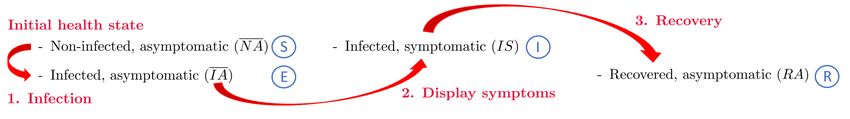
1. Health states. As shown in Figure 4 we relabel these states in order to make a later distinction in terms of
testing and quarantine. These we call health states. We also allow for the possibility that the exposed state is
infectious, that is that there is possibly asymptomatic transmission.
i. Non-infected, Asymptomatic ( N A) - Individuals that have not been exposed to the virus, and are by
definition asymptomatic. This corresponds to S in the SEIR model: Susceptible.
ii. Infected, Asymptomatic ( I A) - Individuals that have met an infected individual but are as yet asymp-
tomatic. This corresponds to E in the SEIR model: Exposed. Relative to the SEIR model we allow that
these individuals may also transmit the virus albeit at a lower frequency.
iii. Infected, Symptomatic ( IS) - Individuals that have met an infected individual and are now showing
symptoms. This corresponds to I in the SEIR model: Infectious.
8iv. Recovered, Asymptomatic ( RA) - Infected individuals that have entered the recovery phase and are
no longer infected. As in the textbook SEIR model we assume these individuals are immune.9 This
corresponds to R in the SEIR model: Recovered.
Figure 4: Transmission and the relationship between our model and the SEIR model
Notes: This figure shows how our states map into the SEIR model. To understand the role of testing we group the asymptomatic states S, E and
label these Non-infected,Asymptomatic (NA) and Infected, Asymptomatic (IA). Without testing, authorities nor individuals are able to differentiate
between these states. To denote this lack of information, we put a bar over them: N A, I A. Exposed individuals show symptoms, which is the I
state of the SEIR model. We label this Infected, Symptomatic (IS). Individuals may then recover, which is the R state of the SEIR model. We label
this Recovered, Asymptomatic (IA).
Figure 5: SEIR model with incomplete information and testing of asymptomatic individuals
Notes: This figure augments Figure 4 to show how we extend the SEIR model to accommodate testing and incomplete information. We add
two additional states that can be revealed by testing, which differentiate asymptomatic individuals { N A, I A}. We denote these with a tilde:
If
A for identified infected, asymptomatic cases, and N g A for identified non-infected, asymptomatic cases. We assume that symptomatic cases
IS are instantly identifiable so are known positives, and that recovered cases have been tracked such that RA cases are known negatives.
Figure 4 tracks an individual case through these states. In terms of medical transmission, we assume that
infected individuals are contagious, although with different rates of transmission. The different rates of trans-
mission nest the case that only IS individuals can transmit the disease, which is the case in the SEIR model.
Non-infected individuals cannot transmit the disease { N A, RA}.
The medical block of the model is very simple and could be enriched in many ways.10 Following the standard
SEIR model: (i) infected asymptomatic individuals show symptoms at rate δ, (ii) infected, symptomatic
9 To the best of our knowledge there is no empirical evidence regarding immunity following COVID-19. A quantitative version of this
model would want to take this into account. This is not the point of departure studied in this paper.
10 See http://gabgoh.github.io/COVID/index.html by Gabriel Goh for an example of an SEIR model of Transmission Dynamics that appends
a rich model of Clinical Dynamics which models hospitalization, length of hospital stay, and more. These states would intercede between IS,
RA and D, which is not the focus of this paper.
9individuals recover at rate ω R and die at rate ω D . Note that all individuals that become infected show
symptoms at some point, this could be relaxed.
2. Incomplete information. We allow for incomplete information, as described in Figure 5. In terms of policy,
we assume that unless tested, individuals without symptoms are indistinguishable and so must be treated
in the same way by quarantine policy. To achieve this we distinguish between two types of N A and I A
individuals. Adding these new cases in green to Figure 4 gives Figure 5. In the first case the diagnosis
regarding infection is unknown. These are unknown cases which we denote N A and I A. In the second case
the diagnosis regarding infection is known, which we denote N
g A and If
A. This information structure implies
that testing and quarantine policies can not distinguish between the following pairs of cases: unknown cases
{ N A, I A}, known positives { If
A, IS}, and known negatives { N
g A, RA}. Our assumption that { N gA, RA} are
not distinguishable is a simplifying assumption in order to maintain a finite set of states, which we discuss
below.
3. Meeting and transmission rates. We assume that the underlying parameters consist of an explicit interaction
of social meeting rates, which are mutable to quarantine / social distancing policies, and medical transmission
rates, which are the medical rates of transmission between two individuals that meet.
We denote quarantine and non-quarantine states by Q and NQ, respectively. Interacted with our 4 health
states, plus two additional information states, this gives 12 total states that individuals can be in. The meeting
rates of non-quarantined individuals is given by λ, and for quarantined individuals by λQ . We interpret the
ratio factor by which quarantine reduces the rate of social interaction (λ/λQ ) as the quarantine technology and
treat it as a parameter.
We denote the transmission rates by ρ A ρS for asymptomatic (symptomatic) cases to accommodate evidence
that transmission rates are higher in symptomatic cases. These give the probability that, conditional on
meeting an infected case ( I A, If
A, IS), a non-infected individual ( N A, N
g A) becomes infected. Crucially, in-
dividuals do not know who is infected, and do not know that they have met an infected person.11
4. Testing. We introduce a role for testing. Our information structure has assumed that when symptoms
present, the individual and society know that the individual is infected. In this paper we do not cover
testing of symptomatic individuals, although this is obviously a hugely important area.12 We assume that
testing of asymptomatic individuals takes place at a rate τ. Testing fully reveals an individual’s health state.
Tests do not produce false negatives or false positives.
An issue arises in that individuals who have previously tested negative can become infected. This would
require them to transition to either If
A or I A. If we assume either, then they move into a different group for
11 This seems like a reasonable assumption to us despite one of the requisites for testing in many countries being that individuals can identify
an infected individual that they interacted with.
12 Note that in our model if we were to test symptomatic individuals then all tests would yield positives. In the data a small fraction of tests
yield positives. In the US our interpretation of this is not that the US is testing asymptomatic people, but rather that individuals with similar
symptoms due to common colds and the flu are being tested. To introduce testing of symptomatic individuals one would really want to extend
the model to introduce an additional disease that presents observationally identical symptoms that can then be separated by testing.
10the purpose of policy. However the transition would not be observed since the individual remains asymp-
tomatic. Addressing this completely would require significantly enriching the model.13 To avoid this, and
in the spirit of this paper being a first step, we assume that testing has a ‘tagging’ property, such that the
transition from N gA to If
A is observed. We highlight this in the notes to Table 3.
5. Conditional quarantine. We allow for quarantine policy and restrict this to depend on the observable health
state of the individual. To keep the Markovian structure of the SEIR model, we quarantine individuals at
constant rates. When there is no testing, individuals are moved from non-quarantine ( NQ) to quarantine ( Q)
at rates ξ u , ξ + , ξ r , for unknown, known positive and recovered cases. When there is testing, individuals are
moved from non-quarantine ( NQ) to quarantine ( Q) at rates ξ u , ξ − , ξ + , ξ r , for unknown, known negative,
known positive, and recovered cases, where now the known positive cases include If A individuals. We
assume a set of corresponding rates at which individuals are released from quarantine: r u , r − , r + , rr .
3.2 Transmission
Given the above description of the model, we now describe transition rates of individuals between states. We
work in continuous time and when simulating the model we consider a discrete time approximation in which a
period is one hour and days are 14 hours long.
States. Individuals in the model are in one of 13 states:
- {Non-infected & Asymptomatic}×{Quarantine, Non-quarantine}×{Unknown, Known negative} → 4 states
- {Infected & Asymptomatic}×{Quarantine, Non-quarantine}×{Unknown, Known positive} → 4 states
- {Infected & Symptomatic} ×{Quarantine, Non-quarantine} → 2 states
- {Recovered & Aymptomatic} ×{Quarantine, Non-quarantine} → 2 states
- Deceased → 1 state
There is initially a distribution of a unit mass of individuals. When we simulate the model, we will assume that
these individuals are non-quarantined, asymptomatic and unknown cases, with a small number being infected:
N A, NQ and I A, NQ. We denote the mass of individuals in a state X in period t by MtX .
Social interaction. In order to transmit the disease, individuals must first meet. We assume random matching.
Non-quarantined individuals meet other individuals at rate λ, while quarantined individuals meet others at rate
λQ . To save on notation we use, for example, N A to denote both N A and N
g A when distinguishing between the
two is not relevant.
13 A richer model would include something like the following. Individuals tests are viewed as ‘good’ for some number of days. Policies
may therefore apply to individuals who were tested in, say, the ‘last 60 days’. It is understood that some of these individuals would become
infected and this would not be observed unless re-tested or symptoms develop. Given the law of large numbers, one could write down the
law of motion for the fraction of ‘tested negatives’ that have since become positive. In this model individuals would require re-testing to keep
track of the pandemic, a clear necessary extension of this model in order to use it quantitatively.
11The conditional probabilities of meetings are as follows. The mass of individuals that are out in the world to
bump into is given by Mt , and depends on the mass of individuals that are quarantined and non-quarantined:
Mt = λMtNQ + λQ MtQ .
The masses of non-quarantined and quarantined individuals are given by:
MtNQ = MtN A,NQ + MtI A,NQ + MtIS,NQ + MtRA,NQ ,
MtQ = MtN A,Q + MtI A,Q + MtIS,Q + MtRA,Q .
Conditional on meeting an individual, the probability that the individual is infected (non-infected) is given by πtI
πtN :
h i h i
MtI λMtI,NQ + λQ MtI,Q λ MtI A,NQ + MtIS,NQ + λQ MtI A,Q + MtIS,Q
πtI = = = ,
Mt Mt Mt
h i h i
MtN λMtA,NQ + λQ MtA,Q λ MtN A,NQ + MtRA,NQ + λQ MtN A,Q + MtRA,Q
πtN = = = .
Mt Mt Mt
Conditional on meeting an infected individual, the probability that the infected individual is symptomatic (asymp-
tomatic) is given by πtI A πtIS :
λMtI A,NQ + λQ MtI A,Q λMtIS,NQ + λQ MtIS,Q
πtI A = , πtIS = .
MtI MtI
Infection. When individuals meet an infected individual, they become infected with probability ρ A ρS if the
individual they meet is asymptomatic (symptomatic). Once infected, an individual does not know that they are
infected as they are initially asymptomatic. A test, which occurs at rate τ, would reveal that they are infected, and
the subject to quarantine policies of infected individuals. We assume that infected individuals all show symptoms
and do not transition straight to a recovery.14 Infected, asymptomatic, individuals show symptoms at a rate δ.
Infected symptomatic individuals then recover at rate ω R and die at rate ω D . Recovered individuals gain complete
immunity in our experiments.
Transmission rate. Combining the above, the rate of infection of a quarantined (non-quarantined) person is given
by λQ αt , (λαt ), where αt is the probability of infection conditional on a random meeting:
h i
αt = πtI πtIS ρS + πtI A ρ A .
14 This is to avoid the issue of having recovered individuals that do not know that they were ever infected. We plan to extend this later on.
The issue with this possibility is that we proliferate the state-space, adding a new state of Recovered, Uninformed, Asymptomatic. This will be
different to Non-infected, Uninformed, Aysmptomatic, due to the different immunity properties of the Recovered individual. Such a recovered
individual can then become infected, and so on and so forth, creating infinitely many states. Our assumption that all infected individuals
eventually know that they are infected by showing symptoms, and then know that they have recovered keeps the state-space finite while still
allowing for the key addition of asymptomatic transmission and incomplete information.
12Note that the infection rate can be written
ρA
S
λαt = ρ λ × πtI πtIS + πtI A .
ρS
Data on the rate of transmission alone will be insufficient to separately identify ρS and λ, although below we
discuss how variation in quarantine policy may be able to estimate these separately in future research.
3.3 Transition rates
As an example of the mechanics of the model, we describe the full set of transition rates for non-infected asymp-
tomatic individuals, and infected asymptomatic individuals. These are the two cases that can be distinguished by
testing asymptomatic individuals. Table 3 provides transition rates between all 13 states. Along with initial condi-
tions for the distribution of individuals across health and information states is sufficient to simulate the model.
3.3.1 Non-infected, asymptomatic individuals
We consider this state as all non-infected individuals in the model are assumed to begin in one of these states.
There are four possible states for non-infected, asymptomatic individuals. They can be an unknown or known
negative case, and they can be non-quarantined or quarantined.
1. Consider an individual that is an unknown case and non-quarantined: N A, NQ.
– Quarantine - At rate ξ u they take up quarantine and transition to N A, Q
– Infection - At rate λ they meet a random individual. With probability πtI πtIS πtI πtI A that individual
is infected and symptomatic (asymptomatic). The individual then becomes I A, NQ with probability
ρS ρ A depending on who the meeting is with. The total transition rate to I A, NQ is therefore λαt .
– Testing - At rate τ, they are tested and since tests are perfect, learn they are not infected, so transition to
being a known negative case: N g A, NQ.
2. Consider an individual that is an unknown case and quarantined: N A, Q.
– Quarantine - At rate r u they are released from quarantine and transition to N A, NQ.
– Infection - The rate of infection is lower in quarantine: λQ αt ≤ λαt .
– Testing - At rate τ, they are tested, learn they are not infected, and transition to being a known negative
case: N
g A, Q.
3. Consider an individual that is a known negative case and non-quarantined: N
g A, NQ
– Quarantine - Since they are recognized as a negative case they may be quarantined at a lower rate
ξ − ≤ ξ u . A policy of indiscriminate quarantine would have ξ − = ξ u . A policy that allows negative
cases to circulate would have ξ − = 0.
13– Infection - The individual still becomes infected at rate λαt and in this case becomes an known infected,
asymptomatic case: If A, NQ.
4. Consider an individual that is a known negative case and quarantined: N
g A, Q
– Quarantine - Since they are recognized as a negative case they may be released from quarantined at a
higher rate r − ≥ r u . A policy of indiscriminate quarantine would have r − = r u . A policy that allows
negative cases to circulate would have r − = 1.
– Infection - The rate of infection is now reduced to λQ αt
3.3.2 Infected, asymptomatic individuals
For brevity we consider the case only for non-quarantined individuals.
1. Consider an individual that is a unknown case: I A, NQ
– Quarantine - Since they are also unknown cases, the rate of quarantine is the same that which must
face N A, NQ individuals. At rate ξ u they transition to quarantine: I A, Q .
– Infection - Since they are already infected there is no transition to infection.
– Testing - At rate τ, they are tested and since tests are perfect, learn they are not infected, so transition to
being a known positive case: I A, NQ.
2. Consider an individual that is a known positive case: If
A, NQ
– Quarantine - Since this is a known case then it can be subjected to the same rate of quarantine as
infected, symptomatic cases. At rate ξ + they transition to quarantine: If
A, Q .
– Infection - Since they are already infected there is no transition to infection.
– Testing - Since they are already tested there is no further testing.
3.3.3 Transition rates between all states
Using the above logic and the structure of the model we can construct the matrix of flows between all 12 active
states and into the deceased state. Table 3 describes all such transition rates.
3.3.4 Nesting the SEIR and SIR models
The SEIR model is nested in our model under the following parameter restrictions.
- No quarantine: λ/λQ = 1
- No asymptomatic transmission: ρ A /ρS = 0
- No testing: τ = 0
In this case individuals move from N A → I A → IS → RA, which correspond to the SEIR states. To obtain the
SIR model, additionally set δ = 1, such that infectiousness is immediate.
14A. Initial state B. Next instant states
Non-infected, Asymptomatic Infected, Asymptomatic Infected, Symptomatic Recovered Dead
N A, NQ N A, Q N
g A, NQ N
g A, Q I A, NQ I A, Q If
A, NQ If
A, Q IS, NQ IS, Q RA, NQ RA, Q D
NA N A, NQ ξu τ λαt
N A, Q ru τ λ Q αt
N
g A, NQ ξ− λαt
N
g A, Q r− λ Q αt
IA I A, NQ ξu τ δ
I A, Q ru τ δ
IfA, NQ ξ+ δ
r+
15
IfA, Q δ
IS IS, NQ ξ+ ωR ωD
IS, Q r+ ωR ωD
R RA, NQ ξr
RA, Q rr
Table 3: Transition rates between health and information states
Notes: This table gives the transition rates between states. Note that in any instant only one transition can occur. For example, an individual that is infected and asymptomatic
and not quarantined may transition to symptomatic and quarantined, but not to symptomatic and not-quarantined. The individual then may transition from symptomatic and non-
quarantined into quarantine. Blue terms refer to policies applied to unknown cases. Red terms refer to policies applied to known positive cases. Green terms refer to policies applied
to known negative cases. The Pink terms are the result of the testing-as-tagging assumption: once tested and known negative, the transition to infection is observed so the individual
becomes a known positive.3.4 Measurement
3.4.1 Basic reproduction number
Consider a hypothetical ‘date-zero’ case. An individual is in the state I A, NQ, while the rest of the population
is in N A, NQ and there are no quarantine procedures in place. A summary statistic of the transmission rate is
the expected number of infections caused by this single infected person: R0I A,NQ . We can state this recursively
as follows. At rate δ the individual becomes symptomatic, which will change their medical transmission rate to
ρS ≥ ρ A :15
R0I A,NQ = λρ A + (1 − δ) R0I A,NQ + δR0IS,NQ
R0IS,NQ = λρS + 1 − ω R − ω D R0IS,NQ .
This implies that
ρS ρS λ ρ A
δ
R0IS,NQ = λ , R0I A,NQ = + (1)
ωR + ωD δ ρS ωR + ωD
The nested case of the SIR model, which removes the exposed state, is obtained by setting δ = 1 and has a transmis-
sion rate R0 = ρλ/ ω D + ω R .
We can try to use data on transmission rates from Wuhan to bound the effectiveness of quarantine. We view
the Wuhan response as a quarantine everyone policy. If everyone is quarantined then
ρS λ Q ρA
δ
R0I A,Q = + R
δ ρ S ω + ωD
therefore the relative rates of transmission pre- and post-quarantine policy are informative of λ/λQ which is our
. .
measure of the quarantine technology: λQ λ = R0I A,Q R0I A,NQ . In Wuhan, R0I A,NQ = 3.86, while post qurantine
measures leads toR0I A,Q = 0.32. The Wuhan quarantine technology delivers λQ /λ ≈ 0.10. We therefore view this as
an upper bound on the quarantine technology in the United States: (λQ /λ)US ∈ [0.10, 1.00].
3.4.2 Measures of activity
To summarize some of our results we construct five metrics: Output, symptomatic infection, reported cases, mor-
tality and social well-being.
Output. A reasonable approximation of economic activity is that it scales with the number of non-quarantined
workers. We further assume that quarantined workers are Arel ∈ [0, 1) less productive than non-quarantined
workers, and that symptomatic workers do not produce. We therefore define output Yt as
Yt = MtN A,NQ + MtI A,NQ + MtRA,NQ + Arel MtN A,Q + MtI A,Q + MtRA,Q .
15 In the case where ρ I = ρ A and the transition from asymptomatic to symptomatic is instantaneous—i.e. as in the SIR model—then we
have the recursion R0 = λρ + 1 − ω D − ω R R0 which gives R0 = λρ/ ω D + ω R .
16In the initial period all individuals are non-quarantined, so Y0 = 1. Therefore Yt is in units of the percent change
in output from the initial period.
Symptomatic infection. A reasonable approximation of the load on the hospital system is that it scales with the
number of infected, symptomatic individuals. We therefore define hospital load Ht as
Ht = η H MtIS .
We do not consider a richer model of the rate of hospitalization of symptomatic cases, or the incidence of intensive
care. Empirical evidence suggests around 20 (5) percent of symptomatic cases require hospitalization (intensive
care). One could enrich the model such that mortality rates depend on Ht due to congestion and lack of resources,
but this is not the focus of this paper. We therefore present results as the percentage change in Ht period-on-period,
which subsumes linear scaling.
Testing and reported cases. Cases are reported when an asymptomatic infection case is tested, which occurs at
rate τ, or the instant an asymptomatic infection becomes symptomatic, which occurs at rate δ. Give Rt = 0, then
∆Rt = (τ + δ) MtI A .
We also track the number of tests. Initial tests are zero Tt = 0 and then
∆Tt = τ MtN A + MtI A .
Mortality. Since the death state is absorbing total mortality is simply Xt = MtD . In our counterfactuals we con-
sider combinations of testing and quarantine policies that keep this number at the end of the pandemic constant,
and compare the implications for symptomatic infections and output.
Social well-being. We consider a measure of social interaction. Non-quarantined individuals interact and we
add up these meetings each period to get a measure of social interaction. There are MtNQ individuals that are
non-quarantined, in various health states. The rate at which these individuals meet non-quarantined individuals
is λπtNQ , where πtNQ = λMtNQ /(λMtNQ + λQ MtQ ). Therefore our period t measure of social well-being is
λMtNQ
!
St = λMtNQ × .
λMtNQ + λQ MtQ
The upper bound for St is given by a virus-free society in which all individuals are non-quarantined, so S0 = λ.
The lower bound for St is zero, which occurs when all individuals are quarantined.
17Parameter Source / Target Value
A. Known medical .
Rate at which infected become symptomatic δ 6 days incubation period 1 6
.
Relative rate of asymptomatic transmission ρ A ρS No current evidence 1
.
Recovery ωR 14 day recovery period 1 14
Mortality ωD Mortality rate of 1 percent 0.01/0.99 × ω R
B. Calibrated
Rate of meeting λ Normalized contact rate 1
Rate of transmission ρS Given λ, gives R0I A,NQ = 2.5 0.0091
C. Policy parameters
Effectiveness of quarantine technology λQ /λ Half of that implied by Wuhan ∆R0 0.5
Testing of unidentified and asymptomatic cases n τ o 25 to 50 times peak US testing rate 0.5% per day
Quarantine rates for observable cases ξu, ξ−, ξ+, ξr See Section 5
n o
Release rates from quarantine for observable cases r u , r − , r + , rr See Section 5
Table 4: Model parameters and values
4 Calibration
4.1 Parameters
Parameter values are given in Table 4. The parameters of the model can be classified intro three groups. The first
relate to ‘known’ medical parameters, which would be the equivalent of technological parameters in an economic
model, and that we can take from the literature that has formed so far. Obviously the extent to which these
parameters are well understood will evolve over time and we may use this information later on. The second
relate to parameters that are similarly technological in that we think that they represent immutable features of the
model, but that we do not have values for and require calibration. The third are policy parameters and relate to (i)
testing rates, (ii) effectiveness of quarantine, (iii) rules for quarantine. We describe these in the next section when
describing our counterfactuals.
Known medical. We assume that the rate at which infected individuals transition from asymptomatic to symp-
tomatic cases, δ, is such that the average incubation period is 6 days (Wu, Leung, and Leung, 2020). World
Health Organization (2020) report that the average recovery period is 14 days for mild infections, we therefore
set ω R = 1/14. There is little data on the relative rates of infection of symptomatic and asymptomatic individu-
.
als.16 We assume a common infection rate: ρ A ρS = 1.
From surveying estimates we target a mortality rate of 1 percent. In the model we denote this by π D , which is
16 https://www.buzzfeed.com/albertonardelli/coronavirus-testing-iceland. “Early results from deCode Genetics indicate that a low pro-
portion of the general population has contracted the virus and that about half of those who tested positive are non-symptomatic”.
18the fraction of individuals experiencing symptoms ( IS) that die. Then
ωD
πD = .
ωR + ωD
We use this to determine ω D given ω R and π D = 0.01.
Unknown and calibrated. We use empirical estimates of the rate of basic transmission and equation (1) to calibrate
λ and ρS . We treat R0I A,NQ
as data, taking the value of 2.5, which is in the middle of the range of empirical
estimates. Using equation (1) provides an equation in two unknowns λ, ρS .
Without further data these parameters cannot be separately identified. We therefore set λ = 1 and back out the
implied ρS that is consistent with (1). To match the same basic rate of transmission requires
R0I A,NQ
ρS = i.
ρA
h
λ δ
δ ρS
+ ω R +ω D
In the future, within-region across-time variation in quarantine measures may allow us to separately identify
λ, ρS . We set the quarantine technology λQ /λ = 0.50.
5 Counterfactuals
Our aim is to provide a small handful of counterfactuals with a minimal set of parameters. The configuration of
these parameters is given in Table 5, and their values are given in Table 6. Section 5 and Section 6 refer to Case 1 in
these tables, we consider Case 2—in which we repeat the exercise under more effective quarantine—in Section 7
Initial conditions. We seed the economy by choosing initial conditions that replicate the U.S. COVID-19 experi-
ence. We assume an initial infected population of 300 individuals and 1 detected case. We measure all model and
data counterparts as of the 100th detected case.
Vaccine. We abstract from the long-run, and instead focus on testing and quarantine in the current phase of the
pandemic. Consistent with this, we assume that in each case a vaccine is introduced to the economy after 500 days.
The vaccine moves individuals in any of the N A states through to RA, NQ state, which makes them immune. The
vaccine rolls out slowly, at a rate of 0.10 percent per day.
n o n o
Counterfactuals. We then consider three different cases for the policy parameters: ξ u , ξ − , ξ + , ξ r , r u , r − , r + , rr ,
τ. We express these parameters as daily rates, despite the model being hourly. With so many parameters we have
many degrees of freedom. We constrain these parameters in a simple way across counterfactuals so that we can
be precise, but others may wish to consider many alternatives. We consider one at the end. Given that we have
19assumed immunity, in all cases we set the quarantine rate of recovered individuals ξ r to zero and their release rate
rr to 1.
Baseline. Our baseline model features no quarantine and no testing. With no testing ξ − and r − are off the table,
since no unknown cases are tested and identified as negative. We then set ξ + = ξ u = 0 and r + = r u = 1.17 This is
the worst-case scenario in which the government does nothing to stop the spread of the virus.
Policy interventions. We consider two policy interventions that capture broad quarantine and targeted quaran-
tine with testing. These policies begin on March 18th, which is two weeks after the first 100 cases are reported in
the data and in the model. Aiming to cut down on parameters, we assume that in both cases known positive cases
are quarantined and not released: ξ + = 1, r + = 0. We therefore have 6 parameters remaining: ξ u and r u in the
quarantine case, and ξ u , ξ − , r u and r − in the testing case.
1. No testing - Common Quarantine. Our first policy is an approximation of what we have observed in the
United States in March, 2020. In this counterfactual there is no testing of asymptomatic individuals and so no
known negative cases. There is therefore a common quarantine rate for all asymptomatic individuals. We set this
rate in counterfactual number 2 to ξ 2u = 0.010, implying a 1 percent per day quarantine rate. This is in line with
the data in Table 2, in which roughly 24 percent of the US population was quarantined within 19 days. We assume
that the rate of release from quarantine is zero.
2. Testing - Targeted quarantine. Our second policy assumes that the government tests asymptomatic individu-
als at a rate τ. While the US is testing at a rate of roughly 0.01 percent of the population per day.18 We assume that
the US increases its testing capacity by roughly 50 fold to τ = 0.5% per day. In levels, this would require testing
1,700,000 asymptomatic people per day, while the US is currently testing around 50,000 symptomatic people per day.
In the spirit of our paper being a proof of concept, we choose for comparison a very simple policy. We maintain
the rate of quarantine of unknown cases and assume that known negatives are not released (r3− − = 0). These
stack the decks against the testing policy having large effects. The only targeted quarantine measure that we take
is to assume that non-quarantined known negative cases are quarantined at rate ξ 3− = ∆ × ξ 2− , with ∆ < 1. We
then choose a value for ∆ such that the policy delivers the same number of total deaths as the common quarantine
policy. This procedure delivers a value of ∆ = 0.20. When testing asymptomatic cases, the rate of quarantine of
known negative cases can be cut by a factor of five without increasing the total number of deaths caused by the
pandemic.
17 Fortechnical reasons, when we set a parameter to 1 we set it to a number > .98 percent per day (effectively 1).
18 Countries like South Korea are testing at a rate of approximately 0.05 percent per day. This comes from reports of South Korean test-
ing capacity of 20,000 per day (https://www.wired.co.uk/article/south-korea-coronavirus) and a population in South Korea of 51.47
million.
20A. Counterfactuals B. Parameters
Quarantine rates Release rates Testing
ξ+ ξu ξ− ξr r+ ru r− rr τ
Baseline - Do nothing 0 0 — 0 1 1 — 1 0
Case 1 - Quarantine technology - λQ /λ = 0.50 - Section 5 & 6
1. No testing - Common quarantine 1 ξu — 0 0 0 — 1 0
2. Testing - Targeted quarantine 1 ξu ∆ × ξu 0 0 0 0 1 τ
Case 2 - Strong quarantine technology - λQ /λ = 0.30 - Section 7
1. No testing - Common quarantine 1 ξu — 0 0 0 — 1 0
2. Testing - Targeted quarantine 1 ψ × ξu 0 0 0 0 0 1 τ
Table 5: Configuration of policy parameters for each counterfactual
Notes: This table gives the configurations of the policy parameters of the model under our three counterfactuals. Recovered individuals are
immune and so never quarantined and always released. In the Baseline case there is no quarantine and no testing. Under the 1. No testing -
Common quarantine policy there is no testing, so uninfected and infected asymptomatic cases cannot be distinguished. Symptomatic cases are
the only known positives, and these are completely quarantined and not released. Unknown cases are quarantined at rate ξ 2u and not released.
Under the 2. Testing - Targeted quarantine policy there is testing of asymptomatic individuals at rate τ > 0. Negative, asymptomatic cases are
distinguished, quarantined at a lower rate, but released at the same rate as unknown cases. Given a value of τ we choose ∆ such that overall
deaths from Cases 1 and 2 are equivalent.
Description Policy parameter Daily rate
1. No testing - Common quarantine
Common quarantine rate ξu 1.0 %
2. Testing - Targeted quarantine
Testing rate τ 0.50 %
Case 1 - Quarantine technology λQ /λ = 0.50
Differential quarantine rate: Known negatives ∆ 0.20
Case 2 - Strong quarantine technology λQ /λ = 0.30
Differential quarantine rate: Unknown cases ψ 0.30
Table 6: Counterfactual parameters
Notes: The parameter ∆ is chosen so that both counterfactuals incur the same total deaths.
6 Results
Figure 6 plots our main results where we compare counterfactuals one and two. Statistics for these are given in
Tables 7, 8, 9, which include the Baseline simulation. Panel A plots the cumulative number of reported cases.
Panel B plots the number of infected, symptomatic cases. Given a constant rate of symptoms requiring medical
21Figure 6: Counterfactuals - Quarantine technology - λQ /λ = 0.50
Notes: The red dotted line corresponds to the counterfactual 1. No testing - Common quarantine. The blue dashed line corresponds to the
counterfactual 2. Testing - Targeted quarantine. Output is total non-quarantined, asymptomatic workers. Output in period zeros is equal to
one since all workers are non-quarantined and asymptomatic.
attention, we can think of Panel B as capturing the number of individuals entering the hospital system. Panel C
plots the cumulative fraction of the population that dies. Panel D plots measured output under the assumption
that non-quarantined individuals produce 50 percent as much as quarantined individuals (Arel = .5).
Cases. Common quarantine is effective at slowing the cumulative number of reported cases. Testing and targeted
quarantine are slightly more effective.
Case load. Panel B plots the fraction of infected symptomatic individuals in the economy. Both counterfactual
policies ‘flatten the curve’ relative to the baseline. The reduction in peak infection load is lower under the testing
policy. If we interpret case load as the stress put on hospital capacity, targeted quarantine with testing generates
the smallest peak load of cases. Common quarantine pushes the peak infection back by about 170 days, whereas
the targeted quarantine with testing tends to put the peak case load back by 250 days, buying an additional quarter
to prepare the medical system. Table 9 reports these statistics.
Deaths. Quarantine is an effective tool at reducing the number of deaths. The current US common quarantine
policy, if continued to be enacted at the same rate (1% of the U.S. population entering quarantine per day), would
22You can also read