COVIDHunter: An Accurate, Flexible, and Environment-Aware Open-Source COVID-19 Outbreak Simulation Model
←
→
Page content transcription
If your browser does not render page correctly, please read the page content below
Bioinformatics
                                                                                                                                                doi.10.1093/bioinformatics/xxxxxx
                                                                                                                                 Advance Access Publication Date: Day Month Year
                                                                                                                                                             Manuscript Category

                                           Subject Section

                                           COVIDHunter: An Accurate, Flexible, and
                                           Environment-Aware Open-Source COVID-19
                                           Outbreak Simulation Model
                                           Mohammed Alser∗ , Jeremie S. Kim, Nour Almadhoun Alserr, Stefan W. Tell,
                                           and Onur Mutlu∗
                                           ETH Zurich, Zurich 8006, Switzerland
                                           ∗ To   whom correspondence should be addressed.
                                           Associate Editor: XXXXXXX
                                           Received on XXXXX; revised on XXXXX; accepted on XXXXX
arXiv:2102.03667v1 [q-bio.PE] 6 Feb 2021

                                           Abstract
                                           Motivation: Early detection and isolation of COVID-19 patients are essential for successful implementation
                                           of mitigation strategies and eventually curbing the disease spread. With a limited number of daily COVID-
                                           19 tests performed in every country, simulating the COVID-19 spread along with the potential effect of each
                                           mitigation strategy currently remains one of the most effective ways in managing the healthcare system
                                           and guiding policy-makers. We introduce COVIDHunter, a flexible and accurate COVID-19 outbreak
                                           simulation model that evaluates the current mitigation measures that are applied to a region and provides
                                           suggestions on what strength the upcoming mitigation measure should be. The key idea of COVIDHunter
                                           is to quantify the spread of COVID-19 in a geographical region by simulating the average number of new
                                           infections caused by an infected person considering the effect of external factors, such as environmental
                                           conditions (e.g., climate, temperature, humidity) and mitigation measures.
                                           Results: Using Switzerland as a case study, COVIDHunter estimates that the policy-makers need to
                                           keep the current mitigation measures for at least 30 days to prevent demand from quickly exceeding
                                           existing hospital capacity. Relaxing the mitigation measures by 50% for 30 days increases both the daily
                                           capacity need for hospital beds and daily number of deaths exponentially by an average of 23.8×, who
                                           may occupy ICU beds and ventilators for a period of time. Unlike existing models, the COVIDHunter
                                           model accurately monitors and predicts the daily number of cases, hospitalizations, and deaths due to
                                           COVID-19. Our model is flexible to configure and simple to modify for modeling different scenarios under
                                           different environmental conditions and mitigation measures.
                                           Availability: https://github.com/CMU-SAFARI/COVIDHunter
                                           Contact: alserm@ethz.ch, omutlu@ethz.ch
                                           Supplementary information: Supplementary data is available at Bioinformatics online.

                                           1 Introduction                                                                   of COVID-19 testing, it is still extremely challenging to detect and isolate
                                           Coronavirus disease 2019 (COVID-19) is caused by SARS-CoV-2 virus,               COVID-19 infections at early stages due to three key issues. 1) It is very
                                           which was first detected in Wuhan, the capital city of Hubei Province in         difficult to accurately identify the initial contraction time of COVID-19
                                           China, in early December 2019 (Du Toit, 2020). Since then, it has rapidly        for a patient. This is because COVID-19 patients can develop symptoms
                                           spread to nearly every corner of the globe and has been declared a pandemic      between 2 to 14 days (or longer in a few cases) after exposure to the
                                           in March 2020 by the World Health Organization (WHO). As of January              new coronavirus (Lauer et al., 2020; Li et al., 2020). This variable delay is
                                           2021, COVID-19 has since resulted in more than 96 million laboratory-            referred to as the virus’ incubation period. 2) The coronavirus genome can
                                           confirmed cases around the world, and has killed nearly 2.2% of the              exhibit rapid genetic changes in its nucleotide sequence, which may occur
                                           infected population. As there are currently no anti-SARS-CoV-2-specific          during viral cell replication, within the host body, or during transmission
                                           drugs or effective vaccines widely available to everyone, early detection        between hosts (Andersen et al., 2020). This genetic diversity affects
                                           and isolation of COVID-19 patients remain essential for effectively curbing      the virus virulence, infectivity, transmissibility, and evasion of the host
                                           the disease spread. As a result, many countries across the world have            immune responses (Phan, 2020; Pachetti et al., 2020; Toyoshima et al.,
                                           implemented unprecedented lockdown and social distancing measures,               2020). 3) The situation becomes even worse as the coronavirus can survive
                                           affecting millions of people. Regardless of the availability and affordability   and therefore remain infectious outside the host, on common surfaces
                                                                                                                            such as metal, glass, and banknotes (both paper and polymer) at room
                                                                                                                            temperature for up to 28 days (Kampf et al., 2020; Riddell et al., 2020).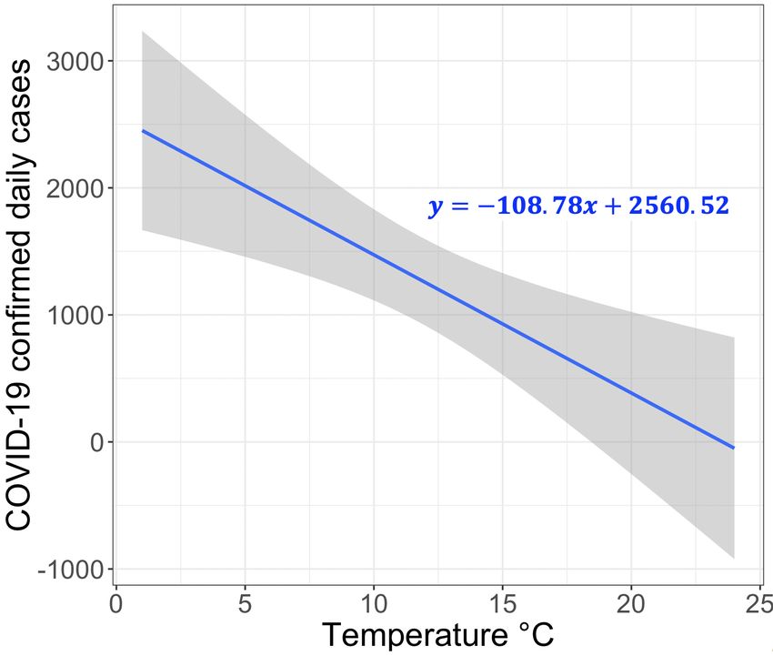
2 Alser et al.
Simulating the spread of COVID-19 has the potential to mitigate should be and for how long it should be applied, while considering
the effects of the three key issues, help to better manage the healthcare the potential effect of environmental conditions. Our model accurately
system, and provide guidance to policy-makers on the effectiveness of forecasts the numbers of infected and hospitalized patients, and deaths for
various (current, planned or discussed) social distancing and mitigation a given day, as validated on historical COVID-19 data (after accounting
measures. To this end, many COVID-19 simulation models are proposed for under-reporting). The key idea of COVIDHunter is to quantify the
(e.g., (Tradigo et al., 2020; Russell et al., 2020; Ashcroft et al., 2020)), spread of COVID-19 in a geographical region by calculating the daily
some of which are announced to assist in decision-making for policy- reproduction number, R, of COVID-19 and scaling the reproduction
makers in countries such as the United Kingdom (ICL (Flaxman et al., number based on changes in both mitigation measures and environmental
2020)), United States (IHME (Reiner et al., 2020)), and Switzerland conditions. The R number changes during the course of the pandemic
(IBZ (Huisman et al., 2020)). These models tend to follow one of two key due to the change in the ability of a pathogen to establish an infection
approaches. (1) Evaluating the current actual epidemiological situation by during a season and mitigation measures that lead to lower number of
accounting for reporting delays and under-reporting due to inefficiencies of susceptible individuals. COVIDHunter simulates the entire population
such as low number of COVID-19 tests. (2) Evaluating the current and of a region and assigns each individual in the population to a stage of the
future epidemiological situation by simulating the COVID-19 outbreak COVID-19 infection (e.g., from being healthy to being short-term immune
without relying on the observed (laboratory-confirmed) number of cases to COVID-19) based on the scaled R number. Our model is flexible to
in simulation. configure and simple to modify for modeling different scenarios as it uses
The first approach, taken by the IBZ (Huisman et al., 2020), only three input parameters, two of which are time-varying parameters, to
LSHTM (Russell et al., 2020), and (Ashcroft et al., 2020) models, is calculate the R number. Whenever applicable, we compare the simulation
not mainly used for prediction purposes as it reflects the epidemiological output of our model to that of four state-of-the-art models currently used
situation with about two weeks of time delay (due to its dependence on to inform policy-makers, IBZ (Huisman et al., 2020), LSHTM (Russell
observed COVID-19 reports). The IBZ model (Huisman et al., 2020) et al., 2020), ICL (Flaxman et al., 2020), and IHME (Reiner et al., 2020).
estimates the daily reproduction number, R, of SARS-CoV-2 from The contributions of this paper are as follows:
observed COVID-19 incidence time series data after accounting for
reporting delays and under-reporting using the numbers of confirmed • We introduce COVIDHunter, a flexible and validated simulation
hospitalizations and deaths. The R number describes how a pathogen model that evaluates the current and future epidemiological situation
spreads in a particular population by quantifying the average number of by simulating the COVID-19 outbreak. COVIDHunter accurately
new infections caused by each infected person at a given point in time. The forecasts for a given day 1) the reproduction number, 2) the number of
LSHTM model (Russell et al., 2020) adjusts the daily number of observed infected people, 3) the number of hospitalized people, 4) the number
COVID-19 cases by accounting for under-reporting (uncertainty) using of deaths, and 5) number of individuals at each stage of the COVID-19
both deaths-to-cases ratio estimates and correcting for delays between infection. COVIDHunter evaluates the effect of different current and
case confirmation (i.e., laboratory-confirmed infection) to death. future mitigation measures on the COVIDHunter’s five numbers.
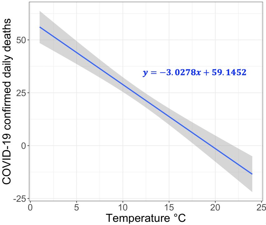
The second approach, taken by ICL (Flaxman et al., 2020) and • As a case study, we statistically analyze the relationship between
IHME (Reiner et al., 2020) models, usually requires a large number of temperature and number of COVID-19 cases in Switzerland. We
various input parameters and assumptions. IHME (Reiner et al., 2020) find that for each 1◦ C rise in daytime temperature, there is a 3.67%
model requires input parameters such as testing rates, mobility, social decrease in the daily number of confirmed cases. We demonstrate
distancing policies, population density, altitude, smoking rates, self- how considering the effect of climate (e.g., daytime temperature) on
reported contacts, and mask use. This model makes two key assumptions: COVID-19 spread significantly improves the prediction accuracy.
1) the infection fatality rate (IFR), which indicates the rate of people that • Compared to IBZ, LSHTM, ICL, and IHME models, COVIDHunter
die from the infection is taken using data from the Diamond Princess Cruise achieves more accurate estimation, provides no prediction delay, and
ship and New Zealand and 2) the decreasing fatality rate is reflective of provides ease of use and high flexibility due to the simple modeling
increased testing rates (identifying higher rates of asymptomatic cases). approach that uses a small number of parameters.
ICL (Flaxman et al., 2020) model requires input parameters such as the • Using COVIDHunter, we demonstrate that the spread of COVID-19 in
daily number of confirmed deaths, IFR, mobility rates from Google, age- Switzerland is still active (i.e., R > 1.0) and curbing this spread requires
and country-specific data on demographics, patterns of social contact, and maintaining the same strength of the currently applied mitigation
hospital availability. This model makes three key assumptions: 1) age- measures for at least another 30 days.
specific IFRs observed in China and Europe are the same across every • We release the well-documented source code of COVIDHunter and
country, 2) the number of confirmed deaths is equal to the true number of show how easy it is to flexibly configure for any scenario and extend
COVID-19 deaths, and 3) the change in transmission rates is a function of for different measures and conditions than we account for.
average mobility trends.
To our knowledge, there is currently no model capable of accurately
monitoring the current epidemiological situation and predicting future 2 Methods
scenarios while considering a reasonably low number of parameters and
2.1 Overview
accounting for the effects of environmental conditions, as we summarize
in Table 1. The low number of parameters provides four key advantages: The primary purpose of our COVIDHunter model is to monitor and
1) allowing flexible (easy-to-adjust) configuration of the model input predict the spread of COVID-19 in a flexibly-configurable and easy-
parameters for different scenarios and different geographical regions, to-use way, while accounting for changes in mitigation measures and
2) enabling short simulation execution time and simpler modeling, 3) environmental conditions over time. We employ a three-stage approach to
enabling easy validation/correction of the model prediction outcomes by develop and deploy this model. (1) The COVIDHunter model predicts the
adjusting fewer variables, and 4) being extremely useful and powerful daily R value based on only three input parameters to maintain both quick
especially during the early stages of a pandemic as many of the simulation and high flexibility in configuring these parameters. Each input
parameters are unknown. Simulation models need to consider the fact parameter is configured based on either existing research findings or user-
that the environmental conditions (e.g., air temperature) affect pathogen defined values. Our model allows for directly leveraging existing models
infectivity (Fares, 2013; Kampf et al., 2020; Riddell et al., 2020; Xu et al., that study the effect of only mitigation measures (or only environmental
2020) and simulating this effect helps to provide accurate estimation of conditions) on the spread of COVID-19, as we show in Section 2.2. (2)
the epidemiological situation. The COVIDHunter model predicts the number of COVID-19 cases based
Our goal in this work is to develop such a COVID-19 outbreak on the predicted R number. COVIDHunter simulates the entire population
simulation model. To this end, we introduce COVIDHunter, a simulation of a region and labels each individual according to different stages of
model that evaluates the current mitigation measures (i.e., non- the COVID-19 infection timeline. Each stage has a different degree of
pharmaceutical intervention or NPI) that are applied to a region and infectiousness and contagiousness. The model simulates these stages for
provides insight into what strength the upcoming mitigation measure each individual to maintain accurate predictions. (3) The COVIDHunter
model predicts the number of hospitalizations and deaths based on bothCOVIDHunter: An Accurate, Flexible, and Environment-Aware Open-Source COVID-19 Outbreak Simulation Model 3
Table 1. Comparison to other models used to inform government policymakers, as of January 2021.
Open Well- Accounting for Low Number Reported
Model Source Documented# Weather Changes of Parameters COVID-19 Statistics
COVIDHunter (this work) 3 3 3 3 3 (R, cases, hospitalizations, and deaths)
IBZ (Huisman et al., 2020) 3 7 7 3 7 (only R)
LSHTM (Russell et al., 2020) 3 7 7 3 7 (only cases)
ICL (Flaxman et al., 2020) 3 3 7 7 3 (R, cases, hospitalizations, and deaths)
IHME (Reiner et al., 2020) 3∗ 7 7 7 7 (cases, hospitalizations, and deaths)
# Based on each model’s GitHub page (all models are available on GitHub). ∗ The available packages are configured only for the IHME infrastructure.
the predicted number of cases and the R number. Next, we explain the et al., 2020). There are currently several studies that demonstrate the
COVIDHunter model in detail. strong dependence of the transmission of SARS-CoV-2 virus on one
or more environmental conditions, even after controlling (isolating) the
2.2 How does the COVIDHunter Model Work? impact of mitigation measures and behavioral changes that reduce contacts.
Several studies have demonstrated increased infectiousness by a country-
The COVIDHunter model predicts the dynamic value of R for a population dependent fixed-rate with each 1◦ C fall in daytime temperature (Xie
at a given day while considering three key factors: 1) the transmissibility and Zhu, 2020; Prata et al., 2020). Another study supports the same
of an infection into a susceptible host population, 2) mitigation measures temperature-infectiousness relationship, but it also finds that before
(e.g., lockdown, social distancing, and isolating infected people), and 3) applying any mitigation measures, a one degree drop in relative humidity
environmental conditions (e.g., air temperature). Our model calculates the shows increased infectiousness by a rate lower (2.94× less) than that of
time-varying R number using Equation 1 as follows: temperature (Wang et al., 2020).
One of the most comprehensive studies that spans more than 3700
R(t) = R0 ∗ (1 − M (t)) ∗ Ce (t) (1) locations around the world is HARVARD CRW (Xu et al., 2020). It finds
the statistical correlation between the relative changes in the R number
The R number for a given day, t, is calculated by multiplying three terms: and both weather (temperature, ultraviolet index, humidity, air pressure,
1) the base reproduction number (R0) for the subject virus, 2) one minus and precipitation) and air pollution (SO2 and Ozone) after controlling
the mitigation coefficient (M ), for the given day t and 3) the environmental the impact of mitigation measures. The study provides a CRW Index that
coefficient (Ce ) for the given day t. has a value from 0.5 to 1.5. The percentage difference between any two
The R0 number quantifies the transmissibility of an infection into a consecutive values provided by the CRW Index represents the effect that
susceptible host population by calculating the expected average number of both weather and air pollutants have on the R number. For example, a drop
new infections caused by an infected person in a population with no prior in the CRW Index by 10% in a given location points to a 10% reduction in
immunity to a specific virus (as a pandemic virus is by definition novel to all the R number due to weather changes and air pollutants. Our model enables
populations). Hence, the R0 number represents the transmissibility of an applying any of these studies by adjusting our environmental coefficient on
infection at only the beginning of the outbreak assuming the population is a given day, as we experimentally demonstrate in Section 3. For example,
not protected via vaccination. Unlike the R number, R0 number is a fixed if the COVIDHunter user chooses to consider the HARVARD CRW study,
value and it does not depend on time. The R number is a time-dependent and the CRW Index shows, for example, a 10% drop compared to its
variable that accounts for the population’s reduced susceptibility. The R0 immediately preceding data point, then the environmental coefficient of
number for the COVID-19 virus can be obtained from several existing COVIDHunter should be 0.9 so that the R value decreases by also 10%.
studies (such as in (Hilton and Keeling, 2020; Chang et al., 2020; Shi Next, we explain how our model forecasts the number of COVID-19 cases
et al., 2020; de Souza et al., 2020; Rahman et al., 2020)) that estimate it based on Equation 1.
by modeling contact patterns during the first wave of the pandemic.
The mitigation coefficient (M ) applied to the population is a time-
dependent variable and it has a value between 0 and 1, where 1 represents
the strongest mitigation measure and 0 represents no mitigation measure 2.3 Predicting the Number of COVID-19 Cases
applied. In different countries, mitigation measures take different forms, COVIDHunter tracks the number of infected and uninfected persons over
such as social distancing, self-isolation, school closure, banning public time by clustering the population into four main categories: HEALTHY,
events, and complete lockdown. These measures exhibit significant INFECTED, CONTAGIOUS, and IMMUNE. The model initially considers
heterogeneity and differ in timing and intensity across countries (Hale the entire population as uninfected (i.e., HEALTHY). For each simulated
et al., 2020; Davies et al., 2020). Quantifying the mitigation measures day, the model calculates the R value using Equation 1 and decides
on a scale from 0 to 1 across different countries is challenging. The how many persons can be infected during that day. The day when
Oxford Stringency Index (Hale et al., 2020) maintains a twice-weekly- the first case of infection in a population introduced is defined by
updated index that takes values from 0 to 100, representing the severity the user. For each newly infected person (INFECTED), the model
of nine mitigation measures that are applied by more than 160 countries. maintains a counter that counts the number of days from being infected to
Another study (Brauner et al., 2020) estimates the effect of only seven being contagious (CONTAGIOUS). Several COVID-19 case studies show
mitigation measures on the R number in 41 countries. We can directly that presymptomatic transmission can occur 1–3 days before symptom
leverage such studies for calculating the mitigation coefficient on a given onset (Wei et al., 2020; Slifka and Gao, 2020). COVID-19 patients can
day after changing the scale from 0:100 to 0:1 by dividing each value of, develop symptoms mostly after an incubation period of 1 to 14 days (the
for example, the Oxford Stringency Index by 100. median incubation period is estimated to be 4.5 to 5.8 days) (Lauer et al.,
The environmental coefficient (Ce ) is a time-dependent variable 2020; Li et al., 2020). We calculate the number of days of being contagious
representing the effect of external environmental factors on the spread after being infected as a random number with a Gaussian distribution
of COVID-19 and it has a value between 0 and 2. Several related viral that has user-defined lowest and highest values. Each contagious person
infections, such as the Influenza virus, human coronavirus, and human may infect N other persons depending on mobility, population density,
respiratory, already show notable seasonality (showing peak incidences number of households, and several other factors (Ferguson et al., 2020).
during only the winter (or summer) months) (Moriyama et al., 2020; We calculate the value of N to be a random number with a Gaussian
Fisman, 2012). The seasonal changes in temperature, humidity, and distribution that has the lowest value of 0 and the highest value determined
ultraviolet light affect the pathogen infectiousness outside the host (Fares, by the user. If N is greater than the R number (i.e., the target number of
2013; Kampf et al., 2020; Riddell et al., 2020; Xu et al., 2020). infections for that day has been reached), further infections are curtailed
However, the indoor environmental conditions are usually well-controlled preventing overestimation of N by infecting only R persons. Once the
throughout the year, where human behavior and number of households contagious person infects the desired number of susceptible persons, the
can be the major contributor to the spread of the COVID-19 (Moriyama status of the contagious person becomes immune (IMMUNE). The immune4 Alser et al.
status indicates that the person has immunity to reinfection due to either 2.5 Model Validation
vaccination or being recently infected (Lumley et al., 2020). We can validate our model using two key approaches. 1) Comparing the
Our model also simulates the effect of infected travelers (e.g., daily
daily R number predicted by our model (using Equation 1) with the daily
cross-border commuters within the European Union) on the value of reported official R number for the same region. 2) Comparing the daily
R. These travelers can initiate the infection(s) at the beginning of the number of COVID-19 cases predicted by our model (using Equation 2)
pandemic. If such infected travelers are absent (due to, for example,
with the daily number of laboratory-confirmed COVID-19 cases. As of
emergency lockdown) from the target population, the virus would die January 2021, we have already witnessed one year of the pandemic, which
out once the value of R decreases below 1 for a sufficient period of time. provides us several observations and lessons. The most obvious source
Both the number and percentage of infected travelers entering a region are of uncertainty, affecting all models, is that the true number of persons
configurable in our model. The percentage of incoming infected travelers that are previously infected or currently infected is unknown (Wilke and
is not affected by the changes in the local mitigation measures, as these Bergstrom, 2020). This affects the accuracy of the reported R number
travelers were infected abroad. since it is calculated as, for example, the ratio of the number of cases for a
Our model predicts the daily number of COVID-19 cases for a given
week (7-day rolling average) to the number of cases for the preceding
day t, as follows: week. Adjusting the parameters of our model to fit the curve of the
number of confirmed cases is likely to be highly uncertain. The publicly-
TIN F (t) UCON (t)
X X available number of COVID-19 hospitalizations and deaths can provide
Daily_Cases(t) = N (n) + N (m) (2) more reliable data.
n=0 m=0
For these reasons, we decide to use a combination of reported numbers
where TIN F is the daily number of infected travelers that is a user- of cases, hospitalizations, and deaths for validating our model using three
defined variable, N () is a function that calculates the number of persons key steps. 1) We leverage the more reliable data of reported number of
to be infected by a given person as a random number with a Gaussian hospitalizations (or deaths) to estimate the true number of COVID-19
distribution, and UCON is the daily number of contagious persons cases using the ratio of number of laboratory-confirmed hospitalizations
calculated by our model. (or deaths) to the number of laboratory-confirmed cases during the second
wave of the COVID-19 pandemic. We assume that the COVID-19 statistics
during the second wave is more accurate than that during the first wave
2.4 Predicting the Number of COVID-19 Hospitalizations because generally more testing is performed in the second wave. 2) We
and Deaths consider a multiplicative relationship between the true number of COVID-
There are currently two key approaches for calculating the estimated 19 cases and that estimated in step 1. In our experimental evaluation
number of both hospitalizations and deaths due to COVID-19: 1) using (Section 3), we use the true number of COVID-19 cases calculated using
historical statistical probabilities, each of which is unique to each age different multiplicative factor values (we refer to them as certainty rate
group in a population (Bhatia and Klausner, 2020; Bi et al., 2020) and 2) levels) as a ground-truth for validating our model. A certainty rate of, for
using historical COVID-19 hospitalizations-to-cases and deaths-to-cases example, 50% means that the true number of COVID-19 cases is actually
ratios (Kobayashi et al., 2020). We choose to follow a modified version double that calculated in step 1. 3) We use our model to calculate both the
of the second approach as it does not require 1) clustering the population daily R number (using Equation 1) and the number of COVID-19 cases
into age-groups and 2) calculating the risk of each individual using the (using Equation 2). We fix the two terms of Equation 1, R0 and Ce , using
given probability, which both affect the complexity of the model and the publicly-available data for a given region and change the third term, M ,
simulation time. until we fit the curve of the number of cases predicted by our model to the
The number of COVID-19 hospitalizations for a given day, t, can be ground-truth plot calculated in step 2. We use the same methodology to
calculated as follows: validate our predicted numbers of hospitalizations and deaths with different
certainty rate levels as we show in Section 3 and the Supplementary Excel
File1 .
Daily_Hospitalizations(t) = Daily_Cases(t) ∗ X ∗ CX (3)
2.6 Flexibility and Extensibility of the COVIDHunter Model
where Daily_Cases(t) is calculated using Equation 2 and X is the
hospitalizations-to-cases ratio that is calculated as the average of daily We especially build COVIDHunter model to be flexible to configure and
ratios of the number of COVID-19 hospitalizations to the laboratory- easy to extend for representing any existing or future scenario using
confirmed number of COVID-19 cases. As the true number of cases is different values of the three terms of Equation 1, 1) R0, 2) M (t), 3)
unknown due to lack of population-scale testing, it is extremely difficult to Ce (t), in addition to several other parameters such as the population,
make accurate estimates of the true number of COVID-19 hospitalizations. number of travelers, percentage of expected infected travelers to the total
As such, we assume a fixed multiplicative relationship between the number number of travelers, and hospitalizations- or deaths-to-cases ratios. Our
of laboratory-confirmed cases and the true number of cases. We use the modeling approach acts across the overall population without assuming
user-defined correction coefficient, CX , of the hospitalizations-to-cases any specific age structure for transmission dynamics. It is still possible to
ratio to account for such a multiplicative relationship. consider each age group separately using individual runs of COVIDHunter
The number of COVID-19 deaths for a given day t can be calculated model simulation, each of which has its own parameter values adjusted
as follows: for the target age group. The COVIDHunter model considers each
location independently of other locations, but it also accounts for potential
movement between locations by adjusting the corresponding parameters
Daily_Deaths(t) = Daily_Cases(t) ∗ Y ∗ CY (4)
for travelers. By allowing most of the parameters to vary in time, t,
the COVIDHunter model is capable of accounting for any change in
where Daily_Cases(t) is calculated using Equation 2 and Y is the transmission intensity due to changes in environmental conditions and
deaths-to-cases ratio, which is calculated as the average of daily ratios of mitigation measures over time. As we explain in Section 2.2, the flexibility
the number of COVID-19 deaths to the number of COVID-19 laboratory- of configuring the environmental coefficient and mitigation coefficient
confirmed cases. The observed number of COVID-19 deaths can still be allows our proposed model to control for location-specific differences in
less than the true number of COVID-19 deaths due to, for example, under- population density, cultural practices, age distribution, and time-variant
reporting. We use the user-defined correction coefficient, CY , to account mitigation responses in each location. Our modeling approach considers
for the under-reporting. One way to find the true number of COVID-19 a single strain of the COVID-19 virus by using a single base reproduction
deaths is to calculate the number of excess deaths. The number of excess
deaths is the difference between the observed number of deaths during time
period and expected (based on historical data) number of deaths during the 1https://github.com/CMU-SAFARI/COVIDHunter/blob
same time period. For this reason, CY may not necessarily be equal to /main/Evaluation_Results/SimulationResultsForSwi
CX . tzerland.xlsxCOVIDHunter: An Accurate, Flexible, and Environment-Aware Open-Source COVID-19 Outbreak Simulation Model 5
number, R0. It is possible to consider multiple virus strains by running Switzerland has increased the daily number of COVID-19 testing by 5.31×
the model simulation multiple times, each of which considers one of the (21641/4074) on average compared to the first wave. We calculate the
strains individually. The model can be extended to consider multiple virus expected number of cases on a given day t with certainty rate levels
strains by replacing the R0 number by multiple R0 numbers that represent of 100% and 50% based on hospitalizations by dividing the number of
the different strains (Reichmuth et al., 2021). hospitalizations at t by X and X/2, respectively, as we show in Figure 1.
We apply the same approach to calculate the expected number of cases on
a given day t with certainty rate levels of 100% and 50% based on deaths
3 Results
using Y and Y /2, respectively.
We evaluate the daily 1) R number, 2) mitigation measures, and 3) Based on Figure 1, we make two key observations. 1) The plot
numbers of COVID-19 cases, hospitalizations, deaths. We also evaluate the for the expected number of cases calculated based on the number of
daily numbers of HEALTHY, INFECTED, CONTAGIOUS, and IMMUNE deaths is shifted forward by 10-20 days (15 days on average) from that
in the Supplementary Excel File2 . We compare the predicted values to for the expected number of cases calculated based on the number of
their corresponding observed values whenever possible. We provide a hospitalizations. This is due to the fact that each hospitalized patient
comprehensive treatment of all datasets, models, and evaluation results usually spends some number of days in hospital before dying of COVID-
with different model configurations in the Supplementary Materials and 19. We do not observe a significant time shift between the plot of the
the Supplementary Excel Files3 . expected number of cases calculated based on the number hospitalizations
and the plot of observed (laboratory-confirmed) cases. 2) The expected
3.1 Determining the Value of Each Variable in the number of cases calculated based on the number of hospitalizations is on
Equations average 1.99× higher than the expected number of cases calculated based
on the number of deaths (after accounting for the 15-day shift) for the same
We use Switzerland as a use-case for all the experiments. However, our certainty rate. This is expected as not all hospitalized patients die.
model is not limited to any specific region as the parameters it uses are We conclude that both numbers of hospitalizations and deaths can be
completely configurable. To predict the R number, we use Equation 1 that used for estimating the true number of COVID-19 cases after accounting
requires three key variables. We set the base reproduction number, R0, for for the time-shift effect.
the SARS-CoV-2 in Switzerland as 2.7, as shown in (Hilton and Keeling, 18000 Expected cases based on hospitalizations (100%)
Expected cases based on hospitalizations (50%)
2020). We choose two main approaches for setting the value of the time- Expected cases based on deaths (100%)
15000 Expected cases based on deaths (50%)
varying environmental coefficient variable (Ce ). 1) Performing statistical Observed cases
Number of COVID-19 Deaths
analysis for the relationship between the daily number of COVID-19 12000
cases and average daytime temperature in Switzerland. As we provide
in the Supplementary Materials, Section 1, our statistical analysis shows 9000
that each 1◦ C rise in daytime temperature is associated with a 3.67%
6000
(t-value = -3.244 and p-value = 0.0013) decrease in the daily number
of confirmed COVID-19 cases. We refer to this approach as Cases- 3000
Temperature Coefficient (CTC). 2) Applying the HARVARD CRW (Xu
et al., 2020) (CRW in short), which provides the statistical relationship 0
Jan-20 Mar-20 May-20 Jul-20 Sep-20 Nov-20 Jan-21
between the relative changes in the R number and both weather factors Date
and air pollutants after controlling for the impact of mitigation measures.
We change the daily mitigation coefficient, M (t), value based on the Fig. 1. Observed (officially reported) and expected number of COVID-19 cases in
ratio of number of confirmed hospitalizations to the number of confirmed Switzerland during the year of 2020. We calculate the expected number of cases based
on both the hospitalizations-to-cases and deaths-to-cases ratios for the second wave. We
cases with two certainty rate levels of 100% and 50%, as we explain in
assume two certainty rate levels of 50% and 100%.
detail in Section 2.5. This helps us to take into account uncertainty in the
observed number of COVID-19 cases, hospitalizations, and deaths. We set
the minimum and maximum incubation time for SARS-CoV-2 as 1 and 5
days, respectively, as 5-day period represents the median incubation period 3.3 Observed and Predicted R number of SARS-CoV-2
worldwide (Lauer et al., 2020; Li et al., 2020). We set the population to We calculate the predicted R number using our model (Equation 1) and
8654622. We empirically choose the values of N , the number of travelers, compare it to the observed official R number and the R number of two
and the ratio of the number of infected travelers to the total number of state-of-the-art models, ICL and IBZ, for the two years of 2020 and
travelers to be 25, 100, and 15%, respectively. 2021. We configure COVIDHunter using the following configurations: 1)
CTC as environmental condition approach, 2) certainty rate levels of 50%
3.2 Evaluating the Expected Number of COVID-19 Cases and 100%, and 3) mitigation coefficient value of 0.7. All our scripts are
for Model Validation provided in our GitHub page. We consider the mean R number provided by
the ICL model. We consider the median R number calculated by the IBZ
As the exact true number of COVID-19 cases remains unknown (due
model based on observed number of hospitalized patients. IBZ provides
to, for example, lack of population-scale COVID-19 testing), we expect
the predicted (after mid of December 2020) R number as the mean of the
the true number of COVID-19 cases in Switzerland to be higher than
estimates from the last 7 days.
the observed (laboratory-confirmed) number of cases. We calculate the
Based on Figure 2, we make three key observations. 1) COVIDHunter
expected true number of cases based on both numbers of deaths and
predicts the changes in R number much (4-13 days) earlier than that
hospitalizations, as we explain in Section 2.5. To account for possible
predicted by ICL model, which leads to a more accurate prediction. The
missing number of COVID-19 deaths, we consider the excess deaths
R number predicted by COVIDHunter (with a certainty rate level of 50%)
instead of observed deaths. We calculate the excess deaths as the difference
is on average 1.56× less than that predicted by ICL model, IBZ model,
between the observed weekly number of deaths in 2020 and 5-year average
and the observed official R number. Using a certainty rate level of 100%,
of weekly deaths. We find that X (hospitalizations-to-cases ratio) and Y
COVIDHunter predicts the R number to be close in value to the observed
(deaths-to-cases ratio, using excess death data) to be 3.526% and 2.441%,
R number. 2) Our model predicts that the current R number is still higher
respectively, during the second wave of the pandemic in Switzerland.
than 1 (1.137 and 1.023 using certainty rate levels of 50% and 100%,
We choose the second wave to calculate the values of X and Y as
respectively) during January 2021. This indicates that the spread of the
SARS-CoV-2 virus is still active and it causes exponential increase in
2 https://github.com/CMU-SAFARI/COVIDHunter/blob number of new cases. 3) Our model predicts that if we keep the same
/main/Evaluation_Results/SimulationResultsForSwi mitigation measure strength as that of January 2021 for at least 30 days
tzerland.xlsx (M(t)= 0.7), then the R number would drop by 18.2% (R= 0.929 and 0.836
3 https://github.com/CMU-SAFARI/COVIDHunter/blob for certainty rate levels of 50% and 100%, respectively). However, if the
/main/Evaluation_Results/ mitigation measures that are applied nationwide in Switzerland are relaxed6 Alser et al.
0.8
by 50% (M(t)= 0.35) for only 30 days (22 January to 22 February 2021),
0.7
0.7
then the R number increases by at least 2.17×.
Mitigation Coefficient M(t)
0.6
We conclude that COVIDHunter’s estimation of the R number is more 0.6
accurate than that calculated by the ICL and IBZ models, as validated by 0.5 0.5
the currently observed R number. 0.4
0.4
0.35
0.3 Oxford Stringency Index
CTC_50%
7 2.5 0.2 CTC_100%
Observed R CRW_50% Monitoring
ICL CRW_100%
6 CTC_50%_M(t)=0.35
0.1 WithoutCTC_50%
CTC_50%_M(t)=0.7 2.0
Reproduction Number, R(t)
CTC_100%_M(t)=0.7 0
5 IBZ Jan-20 Apr-20 Jul-20 Oct-20 Jan-21 Apr-21
Date
1.5
4
Fig. 3. Predicted strength of the mitigation measures (mitigation coefficient, M (t)) applied
3
1.0 in Switzerland from January 2020 to May 2021 provided by Oxford Stringency Index and
2 COVIDHunter. We use two different environmental condition approaches, CRW and CTC.
0.5 We assume two certainty rate levels of 50% and 100%. We use five mitigation M (t) values
1
Monitoring Predicting
of 0.35, 0.4, 0.5, 0.6, and 0.7 for each configuration of our model during 22 January to
0 0.0 22 February 2021. The plot called WithoutCTC_50% represents the evaluation of the
Feb-20 Apr-20 Jun-20 Jun-20 Sep-20 Dec-20 Mar-21 current mitigation measures while ignoring the effect of environmental changes.
Date Date
Fig. 2. Observed and predicted reproduction number, R(t), for the two years of 2020 and
2021. We use CTC environmental condition approach, certainty rate levels of 50% and 3.5 Evaluating the Predicted Number of COVID-19 Cases
100%, and mitigation coefficient values of 0.35 and 0.7 for COVIDHunter. We compare
COVIDHunter’s predicted R number to the observed R number and two state-of-the-art
We evaluate COVIDHunter’s predicted daily number of COVID-19 cases
models, ICL and IBZ. The horizontal dashed line represents R(t) =1.0. in Switzerland. We compare the predicted numbers by our model to the
observed numbers and those provided by three state-of-the-art models
(ICL, IHME, and LSHTM), as shown in Figure 4. We calculate the
observed number of cases as the expected number of cases with a certainty
rate level of 100% (as we discuss in Section 3.2). We use three default
configurations for the prediction of the ICL model: 1) strengthening
3.4 Evaluating the Mitigation Measures mitigation measures by 50%, 2) maintaining the same mitigation measures,
We evaluate the mitigation coefficient, M (t), which represents the and 3) relaxing mitigation measures by 50% which we refer to as
mitigation measures applied (or to be applied) in Switzerland from ICL+50%, ICL, and ICL-50%, respectively, in Figures 4, 5, and 6.
January 2020 to May 2021. We use two different environmental condition We use the mean numbers reported by the IHME model that represents
approaches, CRW and CTC. We assume two certainty rate levels of 50% the most relaxed mitigation measures, called as "no vaccine" by the IHME
and 100% to account for uncertainty in the observed number of cases. model. We use the median numbers reported by the LSHTM model.
We use five mitigation coefficients, M (t), values of 0.35, 0.4, 0.5, 0.6, Based on Figure 4, we make four key observations. 1) Our model
and 0.7 for each configuration of COVIDHunter during 22 January to predicts that the number of COVID-19 cases reduces significantly (less
22 February 2021. We compare the evaluated mitigation measures to that than 600 daily cases) within March 2021 if the same strength of the
evaluated by the Oxford Stringency Index (Hale et al., 2020), as we provide currently applied mitigation measure is maintained for at least 30 days. If
in Figure 3. We also evaluate the mitigation coefficient when we ignore the authority decides to relax the mitigation measures to the lowest strength
the effect of environmental changes (i.e., by setting Ce =1 in Equation 1), that has been applied during the year of 2020 (i.e., M (t) = 0.35), then
while maintaining the same number of COVID-19 cases of that provided the daily expected number of cases increases by an average of 29.6× and
with a certainty rate level of 50%. 23.8× (up to 288,827 daily cases) using the CRW and CTC environmental
Based on Figure 3, we make four key observations. 1) Excluding the approaches, respectively. We provide a comprehensive evaluation for the
effect of environmental changes from the COVIDHunter model, by setting effect of different mitigation coefficient values on the number of cases in the
Ce =1 in Equation 1, leads to an inaccurate evaluation of the mitigation Supplementary Materials, Section 2. 2) COVIDHunter predicts the number
measures. For example, during the summer of 2020 (between the two of COVID-19 cases to be equivalent to that predicted by the IHME model
major waves of 2020), COVIDHunter (WithoutCTC_50%) evaluates the during the second wave with a certainty rate level of 50%. However, during
mitigation coefficient to be as high as 0.6. This means that the mitigation the first wave, the predictions of the IHME model matches the expected
measures (only mandatory of wearing mask on public transport) applied number of cases using a certainty rate level of 100%. This means that,
during the summer of 2020 are only 14% more relaxed compared to the unlike our model, the IHME model considers the laboratory-confirmed
mitigation measures (e.g., closure of schools, restaurants, and borders, cases to be as if the tests are done at a population-scale during the first wave,
ban on small and large events) applied during the first wave, which is which is very likely incorrect. This is in line with a recent study (Ioannidis
implausible. This highlights the importance of considering the effect of et al., 2020) that demonstrates the high inaccuracy of the IHME model. 3)
external environmental changes on simulating the spread of COVID-19. Overall, our model predicts on average 1.7× and 1.9× smaller number of
Unfortunately, environmental change effects are not considered by any of COVID-19 cases than that predicted by ICL model using CTC and CRW
the IBZ, LSHTM, ICL, and IHME models, which we believe is a serious approaches, respectively, and a certainty rate of 50%. This suggests that
shortcoming of these prior models. 2) A drop by 3% (as we observe during the multiplicative relationship between the confirmed number of cases
the mid of November 2020) to 30% (as we observe during the end of August and the true number of cases can be represented by a certainty rate of
2020) in the strength of the mitigation measures for a certain period of time 22% to 33%, which our model can easily account for. The ICL model
(10 to 20 days) is enough to double the predicted number of COVID-19 also shows that there is a sharp drop in the daily number of cases after 13
cases. 3) We evaluate the strength of the mitigation measures applied in November 2020, which corresponds to a 1.6×, 1.4×, and 1.3× increase
Switzerland to be usually (65% of the time) up to 80% to 131% higher in the Oxford Stringency Index, CRW coefficient, and CTC coefficient,
than that provided by the Oxford Stringency Index. 4) The strength of the respectively, applied on 30 October 2020 as we show in Figure 3. 4) The
mitigation measures has changed 11 times during the year of 2020, each number of COVID-19 cases estimated by the LSHTM model during the
of which is maintained for at least 9 days and at most 66 days (32 days on first wave is 1) on average 24% less than that estimated by COVIDHunter
average). and 2) 10 days late from that predicted by COVIDHunter, IHME, and
We conclude that considering the effect of environmental changes (e.g., ICL. The prediction of the LSHTM model during the second wave is not
daytime temperature) on the spread of COVID-19 improves simulation available by the model’s pre-computed projections.
outcomes and provides accurate evaluation of the strength of the past and We conclude that COVIDHunter provides more accurate estimation
current mitigation measures. of the number of COVID-19 cases, compared to IHME (which providesCOVIDHunter: An Accurate, Flexible, and Environment-Aware Open-Source COVID-19 Outbreak Simulation Model 7
3500 Observed Hospitalizations 13000 Monitoring Predicting
CRW_50%_M(t)=0.7
inaccurate estimation during the first wave) and ICL (which provides over- CRW_50%_M(t)=0.35
Number of COVID-19 Hospitalizations
CTC_50%_M(t)=0.7 8500
CTC_50%_M(t)=0.35
estimation), with a complete control over the certainty rate level, mitigation 3000 CTC_100%_M(t)=0.7
IHME 4000
ICL
4000
measures, and environmental conditions. Unlike LSHTM, COVIDHunter ICL+50%
2500 ICL-50%
3500
also ensures no prediction delay.
3000
2000
2500
1500
2000
30000 Expected Cases 305000 Monitoring Predicting
CRW_50%-M(T)=0.7
1000 1500
CRW_50%_M(t)=0.35 175000
CTC_50%_M(t)=0.7
CTC_50%_M(t)=0.35
45000
45000 1000
25000 CTC_100%_M(t)=0.7
Number of COVID-19 Cases
IHME
LSHTM
500
ICL 500
ICL+50%
20000 ICL-50% 36000 0
0
Feb-20 Mar-20 Apr-20 May-20 Sep-20 Nov-20 Jan-21 Mar-21
Date Date
15000 27000
Fig. 5. Observed and predicted number of COVID-19 hospitalizations. We use two different
10000 18000 environmental condition approaches, CRW and CTC with two certainty rate levels of 50%
and 100%. We use two mitigation coefficient values, M (t), of 0.35 and 0.7 for each
5000 9000 configuration of our model during 22 January to 22 February 2021.
0 0
Feb-20 Mar-20 Apr-20 May-20 Sep-20 Nov-20 Jan-21 Mar-21
Date Date 3.7 Evaluating the Predicted Number of COVID-19 Deaths
Fig. 4. Observed and predicted number of COVID-19 cases by our model and other three We evaluate COVIDHunter’s predicted daily number of COVID-19 deaths
state-of-the-art models. We use two different environmental condition approaches, CRW in Figure 6 after accounting for the 15-day shift (as we discuss in
and CTC with two certainty rate levels of 50% and 100%. We use two mitigation coefficient,
Section 3.2). We calculate the observed number of deaths as the number of
M (t), values of 0.35 and 0.7 for each configuration of our model during 22 January to 22
February 2021. excess deaths (Section 2.4) to account for uncertainty in reporting COVID-
19 deaths. Using the number of cases calculated using Equation 2, we
find Y (deaths-to-cases ratio, using excess death data) to be 2.730% and
1.739%, using CRW and CTC, respectively, during the second wave.
3.6 Evaluating the Predicted Number of COVID-19 We make three key observations based on Figure 6. 1) COVIDHunter
Hospitalizations with a certainty rate of 100% predicts the number of deaths to perfectly
fit the three curves of the observed number of excess deaths, ICL deaths,
We evaluate COVIDHunter’s predicted daily number of COVID-19 and IHME deaths, reaching up to 160 hospitalized patients a day. During
hospitalizations in Figure 5. We use the observed official number the second wave, the ICL curve is shifted (late prediction) by 5-10 days
of hospitalizations as is. Using the number of cases calculated with from that of other models. 2) Similar to what we observe for the number of
Equation 2, we find X (hospitalizations-to-cases ratio) to be 4.288% and hospitalizations, our model predicts that the number of COVID-19 deaths
2.780%, using CRW and CTC, respectively, during the second wave. significantly reduces with stricter mitigation measures maintained for at
We make five key observations based on Figure 5. 1) The number of least the upcoming 30 days. Relaxing the mitigation measures by 50%
hospitalizations calculated by COVIDHunter with a certainty rate level (M (t) is changed from 0.7 to 0.35) exponentially increases the death toll by
of 50% matches that calculated by the IHME model. However, IHME an average of 29.6× and 23.8×, reaching up to 7885 new daily deaths, as
model provides a 10-12-day late prediction compared to that provided predicted by COVIDHunter using CRW and CTC environmental condition
by COVIDHunter and the ICL model. 2) The ICL model predicts the approaches, respectively. 3) During the first wave, the use of a certainty rate
number of hospitalizations to be 5× and 7× higher than that predicted by of 50% provides 2.55× and 2.1× (2.36× and 1.52× during the second
COVIDHunter during the first wave (9.3× and 8.1× during the second wave) higher number of deaths compared to that provided by ICL and
wave), using the CTC and CRW approaches, respectively, for evaluating IHME models, when COVIDHunter uses CRW and CTC environmental
the environmental conditions and a certainty rate of 50%. This suggests that condition approaches, respectively.
the ICL model provides 10× and 18.6× higher number of hospitalizations We conclude that 1) unlike the IBZ and LSHTM models,
compared to the observed number of hospitalizations, during first and COVIDHunter is able to predict the number of deaths, 2) COVIDHunter
second waves, respectively, which is highly unlikely and overestimated. predicts the number of deaths to be similar to that predicted by the ICL
3) COVIDHunter with a certainty rate level of 100% predicts the number of and IHME models. Yet, COVIDHunter provides more accurate estimation
cases to perfectly fit the curve of the observed number of hospitalizations, of other COVID-19 statistics (R, number of cases and hospitalizations)
reaching up to 257 hospitalized patients a day. 4) Our model predicts that compared to ICL and IHME, as we comprehensively evaluate in the
the number of COVID-19 hospitalizations reduces with stricter mitigation previous sections, and 3) COVIDHunter requires calculating only the daily
measures maintained for at least 30 days. Relaxing the mitigation measures number of cases and the deaths-to-cases ratio, CY , to predict the daily
by 50% (M is changed from 0.7 to 0.35) exponentially increases the number of deaths.
number of hospitalizations by an average of 29.6× and 23.8×, reaching
up to 12385 new daily hospitalized patients, as predicted by COVIDHunter
450 Observed Excess Deaths 10450
using CRW and CTC environmental condition approaches, respectively. Monitoring Predicting
CRW_50%_M(t)=0.7
400
CRW_50%_M(t)=0.35 5450
This is in line with what the ICL model (ICL-50%) predicts, when ICL CTC_50%_M(t)=0.7
CTC_50%_M(t)=0.35
Number of COVID-19 Deaths
CTC_100%_M(t)=0.7 450
450
model is configured to 50% relaxation in the mitigation measures. 5) The 350 IHME
ICL
ICL+50% 400
use of the CTC approach for determining the environmental coefficient 300 ICL-50%
350
value yields a slightly different number of hospitalizations compared 250
300
to that provided by the use of the CRW approach. This is expected 200 250
as the CTC approach considers only the monthly average change in 200
150
temperature, whereas the CRW approach considers the daily change in 150
100
several environmental conditions. 100
50
We conclude that 1) unlike the IBZ and LSHTM models, 50
COVIDHunter is able to predict the number of hospitalizations and 0 0
Feb-20 Mar-20 Apr-20 May-20 Sep-20 Nov-20 Jan-21 Mar-21
2) COVIDHunter provides more accurate estimation of the number Date Date
of hospitalizations compared to that calculated by ICL (which
Fig. 6. Observed and predicted number of COVID-19 deaths. We use two different
provides overestimation) and IHME (which provides late estimation). environmental condition approaches, CRW and CTC with two certainty rate levels of 50%
COVIDHunter predicts the number of COVID-19 hospitalizations in a and 100%. We use two mitigation coefficient values, M (t), of 0.35 and 0.7 for each
simple, convenient and flexible way that requires calculating only the daily configuration of our model during 22 January to 22 February 2021.
number of cases and the hospitalization-to-cases ratio, CX .8 Alser et al.
4 Summary and Future Work services in the UK: a modelling study. The Lancet Public Health.
de Souza, W. M., Buss, L. F., da Silva Candido, D., et al. (2020). Epidemiological
We demonstrate that we can monitor and predict the spread of COVID-19 and clinical characteristics of the early phase of the COVID-19 epidemic in Brazil.
in an easy-to-use, flexible, and validated way using our new simulation Nature Human Behaviour, 4, 856–865.
model, COVIDHunter. We show how to flexibly configure our model for Du Toit, A. (2020). Outbreak of a novel coronavirus. Nature Reviews Microbiology,
any scenario and easily extend it for different mitigation measures and 18(3), 123–123.
Fares, A. (2013). Factors influencing the seasonal patterns of infectious diseases.
environmental conditions. The use of a small number of variables in our International journal of preventive medicine, 4(2), 128.
model enables a simple and flexible yet powerful way of adapting our Ferguson, N., Laydon, D., Nedjati-Gilani, G., et al. (2020). Report 9: Impact of non-
model to different conditions for a given region. We demonstrate the pharmaceutical interventions (NPIs) to reduce COVID19 mortality and healthcare
importance of considering the effect of environmental changes on the demand. Imperial College London, 10, 77482.
Fisman, D. (2012). Seasonality of viral infections: mechanisms and unknowns.
spread of COVID-19 and how doing so can greatly improve simulation
Clinical Microbiology and Infection, 18(10), 946–954.
accuracy. COVIDHunter flexibly offers the ability to directly make the best Flaxman, S., Mishra, S., Gandy, A., et al. (2020). Estimating the effects of non-
use of existing models that study the effect of one or both of environmental pharmaceutical interventions on COVID-19 in Europe. Nature, 584(7820), 257–
conditions and mitigation measures on the spread of COVID-19. 261.
We benchmark our model against major alternative models of the Hale, T., Petherick, A., Phillips, T., and Webster, S. (2020). Variation in government
responses to COVID-19. Blavatnik school of government working paper, 31.
COVID-19 pandemic that are used to assist governments. Compared to Hilton, J. and Keeling, M. J. (2020). Estimation of country-level basic reproductive
these models, COVIDHunter achieves more accurate estimation, provides ratios for novel Coronavirus (SARS-CoV-2/COVID-19) using synthetic contact
no prediction delay, and provides ease of use and high flexibility due to matrices. PLOS Computational Biology, 16(7), 1–10.
the simple modeling approach that uses a small number of parameters. Huisman, J. S., Scire, J., Angst, D. C., et al. (2020). Estimation and worldwide
monitoring of the effective reproductive number of SARS-CoV-2. medrxiv.
Using COVIDHunter, we demonstrate that the spread of COVID-19 in
Ioannidis, J. P., Cripps, S., and Tanner, M. A. (2020). Forecasting for COVID-19 has
Switzerland (as a case study) is still active (i.e., R > 1.0) and curbing failed. International journal of forecasting.
this spread requires maintaining the same strength of the currently applied Kampf, G., Todt, D., Pfaender, S., and Steinmann, E. (2020). Persistence of
mitigation measures for at least another 30 days. Using COVIDHunter coronaviruses on inanimate surfaces and their inactivation with biocidal agents.
(CTC_100%_M(t)=0.7) on 7 January 2021, we predicted that on 27 Journal of Hospital Infection, 104(3), 246–251.
Kobayashi, T., Jung, S.-m., Linton, N. M., et al. (2020). Communicating the Risk of
January 2021 the number of cases, hospitalizations, and deaths will Death from Novel Coronavirus Disease (COVID-19). Journal of Clinical Medicine,
drop by 19%, 20%, and 30%, respectively. The predicted drop is in 9(2).
line with the observed official number of cases, hospitalizations, and Lauer, S. A., Grantz, K. H., Bi, Q., et al. (2020). The incubation period of coronavirus
deaths (as shown by the Federal Office of Public Health in Switzerland disease 2019 (COVID-19) from publicly reported confirmed cases: estimation and
application. Annals of internal medicine, 172(9), 577–582.
www.covid19.admin.ch) but with different ratios (41%, 59%, and
Li, Q., Guan, X., Wu, P., et al. (2020). Early transmission dynamics in Wuhan, China,
49%, respectively). We believe the difference between the observed and the of novel coronavirus–infected pneumonia. New England Journal of Medicine.
COVIDHunter’s predicted numbers of cases, hospitalizations, and deaths Lumley, S. F., O’Donnell, D., Stoesser, N. E., et al. (2020). Antibody status and
is due to one or more of the following reasons: 1) The lack of population- incidence of SARS-CoV-2 infection in health care workers. New England Journal
scale COVID-19 testing, 2) the use of a more stricter mitigation measure of Medicine.
Moriyama, M., Hugentobler, W. J., and Iwasaki, A. (2020). Seasonality of respiratory
than M (t) = 0.7, and 3) the lack of information about ground truth viral infections. Annual review of virology, 7.
on number of COVID-19 cases, hospitalizations, and deaths. We provide Pachetti, M., Marini, B., Benedetti, F., et al. (2020). Emerging SARS-CoV-2
insights on the effect of each change in the strength of the applied mitigation mutation hot spots include a novel RNA-dependent-RNA polymerase variant.
measure on the number of daily cases, hospitalizations, and deaths. We Journal of Translational Medicine, 18, 1–9.
Phan, T. (2020). Genetic diversity and evolution of SARS-CoV-2. Infection, genetics
make all the data, statistical analyses, and a well-documented model
and evolution, 81, 104260.
implementation publicly and freely available to enable full reproducibility Prata, D. N., Rodrigues, W., and Bermejo, P. H. (2020). Temperature significantly
and help society and decision-makers to accurately and openly review the changes COVID-19 transmission in (sub) tropical cities of Brazil. Science of the
current situation and estimate future impact of decisions. Total Environment, page 138862.
We suggest and plan at least five main directions/additions to further Rahman, B., Sadraddin, E., and Porreca, A. (2020). The basic reproduction number
of SARS-CoV-2 in Wuhan is about to die out, how about the rest of the World?
improve the predictive power and benefits of our COVIDHunter model. 1) Reviews in Medical Virology, page e2111.
Clustering the population based on age-groups. This has potential different Reichmuth, M., Hodcroft, E., Riou, J., et al. (2021). Transmission of SARS-CoV-2
effects on, for example, population, environmental conditions, mitigation variants in Switzerland. https://ispmbern.github.io/covid-19/va
measures (Bhatia and Klausner, 2020; Bi et al., 2020). 2) Considering riants/index.pdf. Accessed: 2021-1-30.
Reiner, R. C., Barber, R. M., Collins, J. K., et al. (2020). Modeling COVID-19
vaccinated persons as another new category of persons in a population.
scenarios for the United States. Nature Medicine.
3) Considering reinfection after immunity (Lumley et al., 2020). 4) Riddell, S., Goldie, S., Hill, A., et al. (2020). The effect of temperature on persistence
Considering the average number of households (or population density), of SARS-CoV-2 on common surfaces. Virology journal, 17(1), 1–7.
as well as other potential population-level effects, while calculating Russell, T. W., Golding, N., Hellewell, J., et al. (2020). Reconstructing the early
the number of new infected persons caused by an infected person. 5) global dynamics of under-ascertained COVID-19 cases and infections. BMC
medicine, 18(1), 1–9.
Considering different strains of the COVID-19 virus by allowing for Shi, Q., Hu, Y., Peng, B., et al. (2020). Effective control of SARS-CoV-2 transmission
multiple base reproduction numbers. Our goal is to update COVIDHunter in Wanzhou, China. Nature medicine, pages 1–8.
with such improvements and capabilities while keeping its simplicity, ease Slifka, M. K. and Gao, L. (2020). Is presymptomatic spread a major contributor to
of use, and flexibility of its modeling strategy. COVID-19 transmission? Nature Medicine, 26(10), 1531–1533.
Toyoshima, Y., Nemoto, K., Matsumoto, S., et al. (2020). SARS-CoV-2 genomic
variations associated with mortality rate of COVID-19. Journal of human genetics,
65(12), 1075–1082.
References Tradigo, G., Guzzi, P. H., Kahveci, T., and Veltri, P. (2020). A method to assess
COVID-19 infected numbers in Italy during peak pandemic period. In 2020 IEEE
Andersen, K. G., Rambaut, A., Lipkin, W. I., et al. (2020). The proximal origin of
International Conference on Bioinformatics and Biomedicine (BIBM), pages 3017–
SARS-CoV-2. Nature medicine, 26(4), 450–452.
3020. IEEE.
Ashcroft, P., Huisman, J. S., Lehtinen, S., et al. (2020). COVID-19 infectivity profile
Wang, J., Tang, K., Feng, K., and Lv, W. (2020). High temperature and high humidity
correction. Swiss Medical Weekly, 150(3132).
reduce the transmission of COVID-19. Available at SSRN 3551767.
Bhatia, R. and Klausner, J. (2020). Estimating individual risks of COVID-19-
Wei, W. E., Li, Z., Chiew, C. J., et al. (2020). Presymptomatic Transmission of
associated hospitalization and death using publicly available data. PloS one, 15(12),
SARS-CoV-2—Singapore, January 23–March 16, 2020. Morbidity and Mortality
e0243026.
Weekly Report, 69(14), 411.
Bi, Q., Wu, Y., Mei, S., et al. (2020). Epidemiology and transmission of COVID-19
Wilke, C. O. and Bergstrom, C. T. (2020). Predicting an epidemic trajectory is
in 391 cases and 1286 of their close contacts in Shenzhen, China: a retrospective
difficult. Proceedings of the National Academy of Sciences, 117(46), 28549–28551.
cohort study. The Lancet Infectious Diseases, 20(8), 911–919.
Xie, J. and Zhu, Y. (2020). Association between ambient temperature and COVID-19
Brauner, J. M., Mindermann, S., Sharma, M., et al. (2020). Inferring the effectiveness
infection in 122 cities from China. Science of the Total Environment, 724, 138201.
of government interventions against COVID-19. Science.
Xu, R., Rahmandad, H., Gupta, M., et al. (2020). The Modest Impact of Weather
Chang, S. L., Harding, N., Zachreson, C., et al. (2020). Modelling transmission and
and Air Pollution on COVID-19 Transmission. medRxiv.
control of the COVID-19 pandemic in Australia. Nature Communications.
Davies, N. G., Kucharski, A. J., Eggo, R. M., et al. (2020). Effects of non-
pharmaceutical interventions on COVID-19 cases, deaths, and demand for hospitalYou can also read