Groundwater Level Prediction for the Arid Oasis of Northwest China Based on the Artificial Bee Colony Algorithm and a Back-propagation Neural ...
←
→
Page content transcription
If your browser does not render page correctly, please read the page content below
water
Article
Groundwater Level Prediction for the Arid Oasis of
Northwest China Based on the Artificial Bee Colony
Algorithm and a Back-propagation Neural Network
with Double Hidden Layers
Huanhuan Li 1 , Yudong Lu 1, *, Ce Zheng 1 , Mi Yang 2 and Shuangli Li 3
 1   Key Laboratory of Subsurface Hydrology and Ecological Effects in Arid Region of Ministry of Education,
     School of Environmental Science and Engineering, Chang’an University, Xi’an 710054, China;
     17742499497@163.com (H.L.); ruudfanschd@139.com (C.Z.)
 2   Shaanxi Yining Construction Engineering Co. Ltd., Xi’an 710065, China; myang1993@163.com
 3   School of Science, Yanbian University, Yanji 133200, China; lpfsmile1991@163.com
 *   Correspondence: luyudong18@163.com; Tel.: +86-176-0298-3162

 Received: 18 January 2019; Accepted: 22 April 2019; Published: 24 April 2019

 Abstract: Groundwater is crucial for economic and agricultural development, particularly in arid
 areas where surface water resources are extremely scarce. The prediction of groundwater levels
 is essential for understanding groundwater dynamics and providing scientific guidance for the
 rational utilization of groundwater resources. A back propagation (BP) neural network based on the
 artificial bee colony (ABC) optimization algorithm was established in this study to accurately predict
 groundwater levels in the overexploited arid areas of Northwest China. Recharge, exploitation,
 rainfall, and evaporation were used as input factors, whereas groundwater level was used as the
 output factor. Results showed that the fitting accuracy, convergence rate, and stabilization of the
 ABC-BP model are better than those of the particle swarm optimization (PSO-BP), genetic algorithm
 (GA-BP), and BP models, thereby proving that the ABC-BP model can be a new method for predicting
 groundwater levels. The ABC-BP model with double hidden layers and a topology structure of
 4-7-3-1, which overcame the overfitting problem, was developed to predict groundwater levels in
 Yaoba Oasis from 2019 to 2030. The prediction results of different mining regimes showed that the
 groundwater level in the study area will gradually decrease as exploitation quantity increases and
 then undergo a decline stage given the existing mining condition of 40 million m3 /year. According
 to the simulation results under different scenarios, the most appropriate amount of groundwater
 exploitation should be maintained at 31 million m3 /year to promote the sustainable development of
 groundwater resources in Yaoba Oasis.

 Keywords: artificial bee colony algorithm; double hidden layers; back-propagation neural network;
 groundwater level prediction; arid oasis

1. Introduction
     The social development and agricultural production of oases in arid regions rely on valuable
groundwater resources. However, the long-term overexploitation of groundwater has continuously
diminished groundwater levels, particularly in arid oases where surface water is extremely scarce
and the ecological environment is fragile [1]. A decline in groundwater levels triggers a series
of eco-environmental problems and seriously affects local agricultural production and economic
development. These problems have been observed in typical oases, such as Yaoba [2], Minqin [3],
and Keriya [4]. Eco-environmental crises caused by the unreasonable utilization of groundwater have

Water 2019, 11, 860; doi:10.3390/w11040860                                        www.mdpi.com/journal/water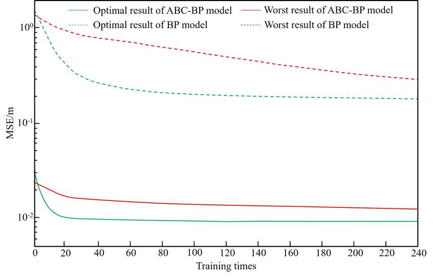
Water 2019, 11, 860 2 of 20
been reported in Northwest China, particularly along the ancient Silk Road, which includes the Hexi
Corridor [5,6], Tianshan Mountains [7], and the edge of the Tarim Basin [8]. The same problems have
been observed in the desert oases of Australia, the United States, and Africa [9–11]. Groundwater level,
which is an important indicator of groundwater balance, exhibits cyclical and random characteristics
under the influences of climatic factors and human activities. Therefore, the accurate prediction of
groundwater level is of great significance for the rational utilization of groundwater resources and the
sustainable development of the social economy in arid areas.
A back-propagation (BP) neural network is a feed-forward and multi-layer network in an artificial
neural network (ANN). Since its introduction, BP has been widely used in evaluation and prediction
due to its strong connection ability and simple structure [12–14]. The accuracy of a BP neural network
depends on the number of hidden layers. Kaveh and Servati (2001) [15] trained a BP neural network for
the design of double-layer grids and observed an improvement in convergence speed and generalization
capability. Neaupane and Achet (2004) [16] demonstrated that a BP neural network with one input
layer, two hidden layers, and one output layer can deliver accurate results when used to predict
slope movement. Métivier (2007) [17] concluded that a BP neural network with two hidden layers
for forecasting stock prices is more accurate than a BP neural network with one, three, four, and five
hidden layers. Haviluddin and Alfred (2014) [18] used a BP neural network with two hidden layers
as a model to simulate network traffic usage and found that the method can obtain an appropriate
mean square error (MSE). Akpinar et al. (2016) [19] accurately predicted natural gas consumption by
using a BP model with two-hidden layers. However, a BP neural network suffers from defects. For
example, this model is sensitive to random initial weights and thresholds, easily becomes trapped in
local minima, and suffers from a slow convergence speed during training. Thus, the traditional BP
neural network should be improved to develop a highly accurate model [20].
The artificial bee colony (ABC) algorithm is a swarm intelligence technology based on the simulated
foraging behavior of honey-bees. The algorithm was proposed by Karaboga for real-parameter
optimization in 2005 and then used to improve BP neural networks and solve local minima and
instability issues in 2007 [21–23]. A BP neural network combined with the ABC algorithm has been
increasingly applied in many fields, such as hydrological evaluation and prediction [24], demand
forecasting [19], and system testing and optimization [25,26]. Many studies have proposed that
the ABC algorithm exhibits a faster convergence rate and more accurate prediction compared with
particle swarm optimization (PSO), genetic algorithm (GA), and ant colony optimization (ACO) [24,27].
In summary, the ABC algorithm, which is equipped with the various ability of the local search and
global convergence, optimizes the initial weights and thresholds of a BP neural network with double
hidden layers to achieve fast convergence performance, improve generalization capability, and avoid
the tendency to fall into a network’s local minima [28–30].
In the current study, Yaoba Oasis was selected as the research area, and groundwater levels
from 2019 to 2030 were predicted under different mining scenarios by developing and training an
ABC-BP model with double hidden layers. This work aims to (i) study the future variation trends
of groundwater levels and find the optimal exploitation quantity for the sustainable development of
agriculture and (ii) provide scientific references for the rational utilization of groundwater resources
and offer novel methodological concepts for similar studies in other arid oases.
2. Materials and Methods
2.1. Study Area
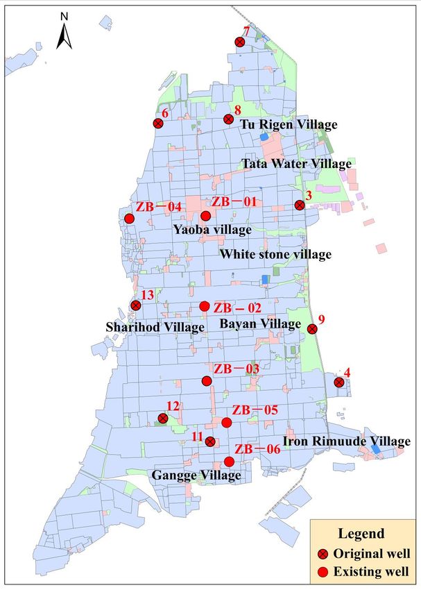
Yaoba Oasis is a typical desert oasis in Northwest China, which is the largest agricultural base of
Alxa in the Inner Mongolia Autonomous Region. Yaoba Oasis lies west of Helan Mountain and east of
Tengger Desert, extending between latitude 38◦ 250 –38◦ 36’ and longitude 105◦ 34’–105◦ 39’ (Figure 1a).
The mean annual rainfall varies between 150 mm and 400 mm from west to east, and the average annual
temperature is 8.29 ◦ C. By contrast, the average annual evaporation ranges from 1400 mm in the east to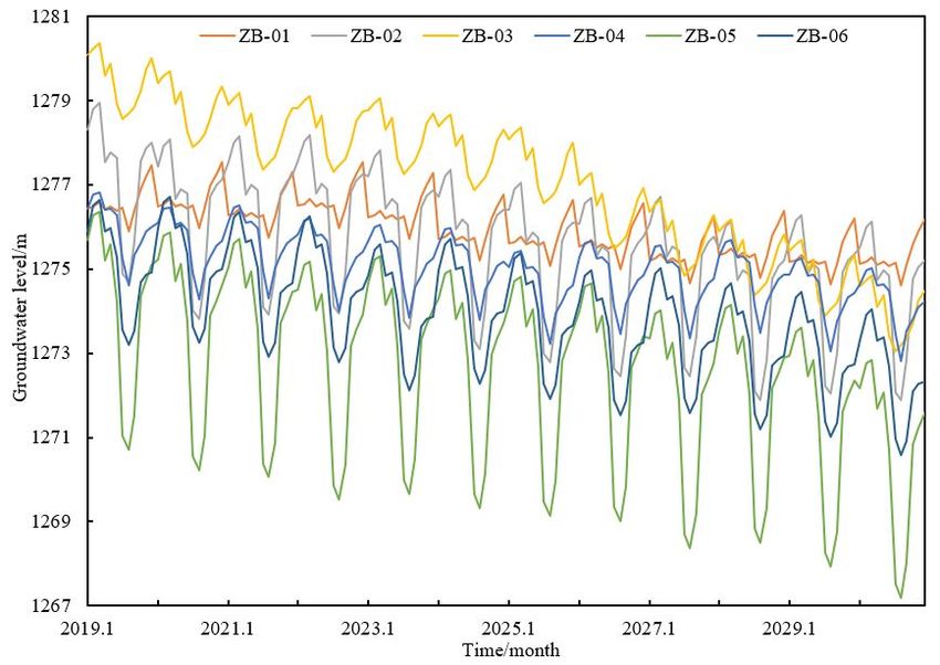
researchers indicate that the total amount of groundwater recharge is maintained at 31 million
m3/year, whereas the amount of groundwater exploitation is maintained at approximately 40 million
m3/year in the study area [31]. Since the development of the oasis in the 1970s, overexploitation has
been observed in the region [32]. Subsequently, groundwater levels have been dropping
continuously      with a cumulative depth of decline that exceeds 12 m [33]. Simultaneously, a series
 Water 2019, 11, 860                                                                                       3 ofof
                                                                                                                20
eco-environmental problems has been triggered, including the contraction of adjacent lakes,
intrusion of groundwater by salt-water, deterioration of groundwater quality, aggravation of soil
 2400 mm in the
salinization,        west. Theof
                 degradation   oasis exhibits a grassland,
                                 surrounding    typical continental  arid climate
                                                            and increase  of land with several characteristics,
                                                                                  desertification; all of these
 namely,   hot   summer   and cold winter, rare rainfall, and intense evaporation. Groundwater
problems seriously influence local economic development, agricultural production, and              haspeoples
                                                                                                        become
 an important
livelihood    [34].water resource for local agricultural production due to the scarce rainfall and extreme
 lack of surface water in Yaoba Oasis. The previous calculations of other researchers indicate that the
 totalData
2.2.   amount
           Sourceofand
                     groundwater
                        Process    recharge is maintained at 31 million m3 /year, whereas the amount of
 groundwater exploitation is maintained at approximately 40 million m3 /year in the study area [31].
      Previous studies have reported that the major factors that influence groundwater levels in
 Since the development of the oasis in the 1970s, overexploitation has been observed in the region [32].
Yaoba Oasis include recharge, exploitation, rainfall, and evaporation, with exploitation as the most
 Subsequently, groundwater levels have been dropping continuously with a cumulative depth of decline
critical influencing factor that exerts the greatest effect [35]. The monitoring data of rainfall and
 that exceeds 12 m [33]. Simultaneously, a series of eco-environmental problems has been triggered,
exploitation are obtained from a local meteorological station, whereas the data of groundwater
 including the contraction of adjacent lakes, intrusion of groundwater by salt-water, deterioration of
levels are derived from six wells of a dynamic monitoring network (Figure 1b). The physical
 groundwater quality, aggravation of soil salinization, degradation of surrounding grassland, and
magnitudes of the data between the four factors and groundwater levels are different. Thus, all the
 increase of land desertification; all of these problems seriously influence local economic development,
data are converted to monthly data, normalized within the range of [–1, 1], and restored to the
 agricultural production, and peoples livelihood [34].
actual predicted values in the prediction model output of the data.

                      (a) Location of study area                   (b) Distribution of observation wells
              Figure 1. Map
                  Figure     of Yaoba
                         1. Map        Oasis,
                                of Yaoba Oasis,Inner
                                                InnerMongolia Autonomous
                                                     Mongolia Autonomous   Region,
                                                                         Region,   China.
                                                                                 China.

2.2. Model
2.3. Data Source
           Setup and Process
       Previous studies have reported that the major factors that influence groundwater levels in Yaoba
2.3.1.
 OasisTopology      of the BPexploitation,
         include recharge,      Neural Network      withand
                                              rainfall,   Double  Hidden with
                                                             evaporation,   Layersexploitation as the most critical
 influencing
      Network  factor  that exerts
                  topology,         the greatest
                              including  the numbereffectof
                                                         [35]. The monitoring
                                                            functional  layers anddata
                                                                                    theofnumber
                                                                                          rainfall of
                                                                                                   and  exploitation
                                                                                                      nodes  in each
 are obtained    from   a local meteorological    station,  whereas  the data  of groundwater    levels
layer, affects the generalization capability and prediction accuracy of the BP neural network [36].      are derived
 fromsame
The     six wells  of a structure
             network     dynamic results
                                    monitoring    network
                                            in different     (Figure for
                                                          outcomes    1b).each
                                                                           Thetraining
                                                                                physicalbecause
                                                                                           magnitudes    of the data
                                                                                                   the weights   and
 between the
thresholds    arefour  factors initialized.
                   randomly     and groundwater       levels are
                                             A BP network     for different.
                                                                  the designThus,   all the datagrids
                                                                               of double-layer     are converted
                                                                                                        was proven to
 monthly data, normalized within the range of [−1, 1], and restored to the actual predicted values in the
 prediction model output of the data.

2.3. Model Setup

2.3.1. Topology of the BP Neural Network with Double Hidden Layers
     Network topology, including the number of functional layers and the number of nodes in each
layer, affects the generalization capability and prediction accuracy of the BP neural network [36].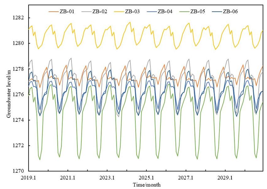
Water 2019, 11, 860                                                                                  4 of 20

The same network structure results in different outcomes for each training because the weights and
thresholds are randomly initialized. A BP network for the design of double-layer grids was proven to
improve generalization performance, overcome over-fitting, and deliver more accurate results than
networks with one, three, four, and more hidden layers [17,37,38]. In the current work, a BP model
with double hidden layers was developed to optimize network structure. The input, first hidden,
second hidden, and output layers belonged to a four-layer working platform of the prediction model.
The input layer was composed of four neuron nodes: recharge, exploitation, rainfall, and evaporation.
The output layer consisted of one neuron node, namely, groundwater level.
     The number of nodes in a hidden layer should be reasonably considered for under-fitting and
over-fitting because these problems can decrease the generalization ability of a network. The error
value of network training increases if the number of nodes in a hidden layer is either too few or too
many. If the number of nodes is excessively few, then the network cannot fully determine the rule for
the sample data, thereby resulting in the inability to establish a complex mapping relationship. In this
case, the BP network exhibits under-fitting and the prediction error is large. By contrast, an excessive
number of hidden nodes will not only make fitting the signal along with the noise easier but will also
extend the learning and training times of the network, thereby resulting in the over-fitting phenomenon
of the network and a large prediction error [39,40]. Selecting the number of hidden layer nodes is a
highly complicated task. To accurately reflect the relationship between the input and the output, the
principle states that fewer hidden layer nodes should be selected to make the network structure as
simple as possible. In this work, the stepwise growing method of a network structure was adopted.
In particular, only a few nodes were first set to train the network and test the learning error. Then, the
number of nodes was gradually increased until the learning error was no longer considerably reduced.
The optimal number of nodes in a hidden layer is commonly determined using Equation (1) [38,41,42].
                                                  √
                                             m = n+l+a
                                             m ≤ 2n + 1
                                                                                                        (1)
                                             m = log2 n
                                                  √
                                             m = nl
where a represents a natural number within [1,10], and m, n, and l represent the nodes of the hidden,
input, and output layers, respectively.
       In the current study, the optimal numbers of nodes in the hidden layer were the range of [3, 9]
calculated using multi-trials algorithms in accordance with the aforementioned formula. The error
of the simulated and measured values in the network training firstly gradually decreased and then
increased with the number of hidden layer neurons increased in Table 1. When the number of nodes
in double hidden layer was set as 7-3, the training of the BP model reached the optimal level with
the minimum error of 0.01. This result indicates the BP neural network with the above construction
can meet the accuracy requirements the and overcome the overfitting problem. Therefore, seven and
three were considered as a reasonable node for the first and second hidden layers, respectively. In the
process of network training, the spatially weighted aggregation and excitation outputs of the input
signal are provided by the seven neuron nodes in the first hidden layer, and the nonlinear mapping
capability of the complex relationship between the input and the output is improved by the three
neuron nodes in the second hidden layer [37]. Accordingly, the network topology of the BP model
with double hidden layers was set to 4-7-3-1 in this work (Figure 2).
       During forward propagation, a neural network receives the sample data and transmits the signal
first to the input layer and then to the output layer after the hidden layer function. If the output results
are consistent with the test samples, then network training is terminated. Otherwise, the weights and
thresholds are repeatedly modified between each layer depending on the back propagation of the error.
Network training is completed when the error of the total samples is less than the pre-set accuracy
requirement [43].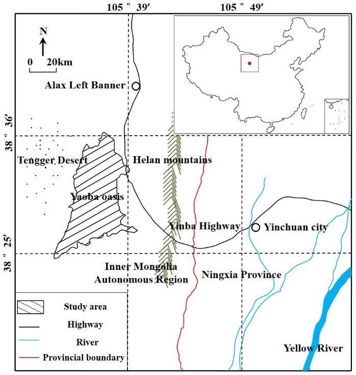
Water 2019, 1, x 5 of 23
3-6Water 2019,
0.70 11, 860
4-6 0.63 5-6 0.23 6-6 0.12 7-6 0.14 8-6 0.29 9-6 5 of 200.38
3-7 0.65 4-7 0.48 5-7 0.20 6-7 0.07 7-7 0.19 8-7 0.34 9-7 0.47
3-8 0.57 4-8 0.45 5-8 0.16 6-8 0.04 7-8 0.25 8-8 0.42 9-8 0.53
3-9 0.52 1. Error
Table 4-9 of network
0.32 5-9
training 0.13different
with 6-9numbers
0.02of nodes
7-9 in the0.29 8-9
first and second 0.46 layers.
hidden 9-9 0.56
Neurons Error
DuringNeurons
forwardError Neurons aError
propagation, neuralNeurons
networkError Neurons
receives Error Neurons
the sample data and Error Neurons
transmits the Error
3-3signal0.86
first to 4-3
the input
0.76layer 5-3
and then
0.57to the6-3output0.34
layer after
7-3 the 0.01
hidden 8-3
layer function.
0.13 If9-3the 0.22
3-4output0.83
results4-4 0.71
are consistent 5-4 the 0.41
with 6-4
test samples, 0.27network
then 7-4 training
0.03 is terminated.
8-4 0.19Otherwise,
9-4 0.26
3-5 0.76 4-5 0.65 5-5 0.38 6-5 0.23 7-5 0.06 8-5 0.24 9-5 0.30
3-6the weights
0.70 and
4-6 thresholds
0.63 are
5-6 repeatedly
0.23 modified
6-6 between
0.12 7-6each layer
0.14 depending
8-6 on
0.29 the back
9-6 0.38
3-7propagation
0.65 of4-7the error.
0.48 Network
5-7 training
0.20 is 6-7
completed
0.07 when7-7
the error
0.19of the8-7
total samples
0.34 is9-7less 0.47
3-8than the
0.57pre-set4-8accuracy
0.45 requirement
5-8 0.16
[43]. 6-8 0.04 7-8 0.25 8-8 0.42 9-8 0.53
3-9 0.52 4-9 0.32 5-9 0.13 6-9 0.02 7-9 0.29 8-9 0.46 9-9 0.56
Back propagation of error
Recharge
Exploitation
Groundwater level
Rainfall
Evaporation
Forward propagation of signal
Input layer First hidden layer Second hidden layer Output layer
Signal flow
Figure 2. Topology chart of the BP neural network with double hidden layers.
Figure 2. Topology chart of the BP neural network with double hidden layers.
2.3.2. Principle of the ABC Algorithm
2.3.2. Principle of the ABC Algorithm
The ABCThe ABC algorithm
algorithm has been haswidely
been widely
appliedapplied to solving
to solving optimization
optimization problems
problems due due
to to
itsits
advantages
advantages of fast convergence and global search. The two core elements of the ABC algorithm are
of fast convergence and global search. The two core elements of the ABC algorithm are bees and food
bees and food sources. The bees are grouped into three types: scout, employed, and onlooker bees.
sources.Scout
The bees
beesarearetasked
grouped into three
to randomly searchtypes:
for thescout, employed,
positions and onlooker
of food sources, bees. Scout
whereas employed and bees are
tasked to randomly
onlooker search
bees are for the
responsible forpositions
mining nectar.of food sources, bees
First, employed whereas employed
mark the and onlooker
size and quantity of a bees
food source and release signals to share the path toward the food source with
are responsible for mining nectar. First, employed bees mark the size and quantity of a food sourceonlooker bees. Then,
onlooker bees commit the food source to their memory and search the neighborhood for a better
and release signals to share the path toward the food source with onlooker bees. Then, onlooker bees
food source by adopting a greedy criterion. Lastly, if the same food source is mined for a certain
commit period,
the food source to their memory and search the neighborhood for a better food source by
then new scout bees find a new food source to replace the current one, thereby maximizing
adopting thea amount
greedyofcriterion.
mined nectar Lastly, if solving
[44]. In the same food source
an optimization is mined
problem, for a certain
the location of a foodperiod,
source then new
scout bees find a new
represents food source
the possible solution,towhereas
replacethe the current
amount one,source
of food thereby maximizing
corresponds to thethe amount
fitness of the of mined
solution
nectar [44]. [21]. Artificial
In solving bees search for
an optimization global artificial
problem, food sources
the location untilsource
of a food an optimal solutionthe
represents is possible
found. In summary, large quantities of food sources, equate to high-quality solutions.
solution, whereas the amount of food source corresponds to the fitness of the solution [21]. Artificial
bees search
2.3.3. for global
ABC-BP artificial
Neural Network food sources until an optimal solution is found. In summary, large
quantities of food sources, equate to high-quality solutions.
2.3.3. ABC-BP Neural Network
A BP neural network is sensitive to random initial weights and thresholds; thus, this neural
network can easily become trapped in local minima and exhibits slow convergence speed during
training [20,22]. The ABC algorithm, which demonstrates local searching and global convergence
abilities, is widely used in training BP neural networks. This algorithm can optimize randomly assigned
weights and thresholds and effectively improve the convergence performance of a network [28–30].
In the current study, the ABC algorithm is adopted to train a BP neural network with double hidden
layers, thereby constructing a new accurate prediction model. The modelling process of the ABC-BP
model is presented as a flowchart in Figure 3. The specific steps are as follows.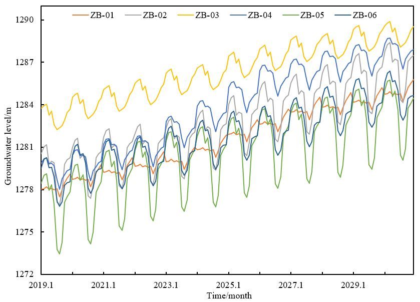
(6) Training is terminated when the cycle number reaches MCN. Otherwise, Step 3 is repeated.
            In this manner, the initial weights and thresholds of the BP neural network are represented by the
            optimal solutions of the ABC algorithm. The cycle number is defined using Equation (8).

                                                          cycle=cycle + 1                                         (8)
Water 2019, 11, 860 (7) The ABC-BP model with double hidden layers is trained and tested with the sample data           6 of 20
            to achieve groundwater level prediction.

                        No          Fitness value:                                    Start
                             new solution > old solution
                                                                                  Construct BP
                     Update
                                            Yes
                    failure +1                                            Initialize parameters of ABC

                         New solution replaces old solution
                                                                                    Cycle=1

                                 Update failure > limit                       Employed bee finds

                           Scout bee finds a new solution                        a new solution

                                                                                 Fitness value:           No
                                 Save optimal solution
                                                                           new solution > old solution
                                                                                        Yes
                                    Cycle=cycle+1
                                                                    New solution replaces old solution
                                                              No
                                 Cycle number=MCN
                                                                                                         Update
                                                                                  Calculate Pi
                                             Yes                                                     failure +1
                          Optimal weights and thresholds
                                                                               Onlooker bee finds
                                   Train and test BP                             a new solution

                 Figure 3. Flowchart
     Figure 3. Flowchart    of the BPof     the BP
                                         neural    neural network
                                                 network  based onbased on the
                                                                    the ABC    ABC algorithm.
                                                                             algorithm.       (modified
                                                                                        (modified from Su et al.,
                 from Su et al., 2012 [24]).
     2012 [24]).
            3. Results and Discussion
      (1) Construct the BP neural network
      Input3.1.
             layer   nodes
                 Model         n (n = 1, 2, . . . , Ninput ), number of hidden layers (Nhidden ), hidden layer nodes
                        Validation
m (m = 1, 2, . . . , Nhidden ), output layer nodes l (l = 1, 2, . . . , Noutput ), training samples p (p = 1, 2, . . . ,
            3.1.1. Initialization of Model Parameters
Ns ), training algorithm, transfer functions among the hidden and output layers, and expected error
are determined. Then, the objective function is established, and the results of this function should be
optimized under the aforementioned conditions [45].
      (2) Initialize the parameters of the ABC algorithm
      The initial parameters of the ABC algorithm include the numbers of solutions (NS ), bee colonies
(NC ), employed bees (Ne ), and onlooker bees (NO ); the maximum cycle number (MCN); and the limit
value. The initial solution Xi (i = 1, . . . , NS ) of the D-dimension vectors is a randomly generated
number within the range of [−1, 1] [27]. NS , NC , Ne , NO , and D satisfy the following relationships:

                                                   NC = 2NS = Ne + NO
                                                                                                                           (2)
                                                   Ne = NO

                          D = Ninput × Nhidden + Nhidden + Nhidden × Noutput + Noutput                                     (3)

where D is the number of optimization parameters; and Ninput , Nhidden , Noutput denote the number of
neurons in the input, hidden, and output layers, respectively [24].
     (3) The algorithm achieves the ideal state when fitness reaches “1”. The fitness value of each
solution is calculated using Equation (4). An artificial employed bee finds a neighboring food source
using Equation (5) and then makes a greedy selection to identify a better solution. If the fitness value
of the new solution is superior to that of the old one, then the old solution is discarded and the new
one is selected. Conversely, the update failure number of the old solution increases by “1” [46].
                                                          (
                                                              1,   MSEi = 0
                                            f ( Xi ) =                                                                     (4)
                                                                1
                                                              MSEi +1 , MSEi >0

                                          Vij = Xij + rand(−1, 1)(Xij − Xk j )                                             (5)
Water 2019, 11, 860                                                                                            7 of 20

where Vij is the value of the jth dimension of the ith solution, f (Xi ) is the fitness value of Vij , i = {1, . . . ,
NS }, j = {1, 2, . . . , D}, k = {1, 2, . . . , NS }, and k,i and k are randomly assigned. MSEi is the MSE of the
ith solution.
      (4) The probability value (Pi ) of the ith solution is expressed as Equation (6). The artificial onlooker
bee searches again (Equation (5)) for a new solution from neighboring solutions in accordance with Pi .

                                                           f ( Xi )
                                                 Pi =                                                             (6)
                                                        Ns
                                                        P
                                                              f ( Xn )
                                                        n=1

     (5) If the update failure number of solutions exceeds the limit, then the solution is discarded.
Subsequently, the employed bee becomes a scout bee that searches randomly for a new solution, which
is generated from the calculation of Equation (7) and stored to replace the old solution [47].

                                     Xi = Xmin + rand(0, 1)(Xmax − Xmin )                                         (7)

     (6) Training is terminated when the cycle number reaches MCN. Otherwise, Step 3 is repeated. In
this manner, the initial weights and thresholds of the BP neural network are represented by the optimal
solutions of the ABC algorithm. The cycle number is defined using Equation (8).

                                                 cycle = cycle + 1                                                (8)

     (7) The ABC-BP model with double hidden layers is trained and tested with the sample data to
achieve groundwater level prediction.

3. Results and Discussion

3.1. Model Validation

3.1.1. Initialization of Model Parameters
     Considering the combination of the ABC algorithm and the BP neural network with double
hidden layers, the ANN function of MATLAB 2014a was used to create and train the ABC-BP model
through programming. The training algorithm of the BP neural network and the transfer functions
of the hidden and output layers exert considerable influences on the accuracy of the prediction
model [38]. Levenberg-Marquardt (“trainlm”), a BP algorithm and training function of the BP neural
network, can effectively shorten the convergence time and improve the convergence performance
of a network compared with other training functions, such as “trainscg”, “traincgp”, “trainrp”, and
“traingdx” [48–50]. The “sigmoid”-type transfer functions of the BP neural network with multiple
hidden layers are commonly used between hidden layers, including “tansig” and “logsig”, and the
linear transfer function “purelin” is typically used between the neurons of the output layer [49]. Many
combined allocations exist among three transfer functions with “tansig”, “logsig”, and “purelin”. The
BP model with double hidden layers can overcome the overfitting problem and achieve the optimal
prediction effect when the algorithm “trainlm” was selected as the training function, the function
“tansig” was selected as the transfer function from the input layer to the first hidden layer, the function
“logsig” was selected as the transfer function from the first hidden layer to the second hidden layer,
and the function “purelin” was selected as the activation function from the second hidden layer
to the output layer [51,52]. The momentum factor, learning rate, maximum number of trainings,
and expected error were set as 0.3, 0.01, 240, and 0.01, respectively. The monthly average recharge,
exploitation, rainfall, and evaporation data from January 2010 to December 2016 were used as input
data. The monthly mean groundwater level data from January 2010 to December 2016 were used
as training samples. The monthly average groundwater level data from January 2017 to December
2018 were used as test samples. Evidently, a large bee colony is equivalent to the identification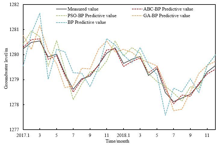
Water 2019, 11, 860 8 of 20
of superior solutions. Nevertheless, this procedure increases the computational complexity of the
algorithm. In the simulation test, the initial numbers of employed bees (Ne ) and onlooker bees (NO )
were set as 100, the number of bee colonies (NC ) was 200, the MCN was 150, and the limit value was
100, which should be greater than the D-dimension of each solution.
3.1.2. Model Training
After the initial parameters were set, the ABC-BP model trained the input data, tested the sample
data several times, and ended the training upon achieving the optimal effect. The analysis result of the
relationship between the fitness value and the cycle number in the training period indicated that the
fitness value rapidly increased with the iteration times during the early stages (Figure 4). This finding
demonstrated that the obtained solution became increasingly optimized. Fitness gradually stabilized
at a constant value after a series of cycles. The result indicated that the model completely converged
when the cycle number reached 150. The training results showed that the convergence rate of the BP
neural network was improved by the ABC algorithm in terms of solving optimization problem.
Water 2019, 1, x 9 of 23
Figure 4. Fitness of solutions in the ABC-BP model.
Figure 4. Fitness of solutions in the ABC-BP model.
As network training was completed, the initial weights and thresholds of the BP neural
As network training
network were wasusing
obtained completed, the initialThe
the ABC algorithm. weights and
weight W thresholds
1 and threshold Bof
1 ofthe
the BP neural
input layer network
to the first
were obtained using hidden layer are
the ABC respectively
algorithm. Thegiven as follows:
weight W1 and threshold B1 of the input layer to the first
hidden layer are respectively given as follows:
−1.831 1.935 0.589 −2.914 −2.271
1.606 2.224 0.485 1.422 −0.554
−1.831 1.935 0.589
0.231 −0.422 -3.011 2.082
−2.914 1.395 −2.271
−0.554
1.606 1 = −2.119
2.224 0.485 1.422 =
W 1.343 0.715 2.321
B1
3.604
0.977
−0.422 1.683−3.011 1.792 1.395
0.231 2.082
-2.318 1.656
W1 = −2.119 1 = 3.604
B 0.965
−2.7681.343 1.475 −1.849
1.705 0.715 2.321
2.6041.683 0.963−2.318
0.406 2.362
−1.416 1.792
0.977 1.656
−2.768 1.705 1.475 −1.849 0.965
The weight W2 and threshold B 2 of the first hidden layer to the
second
hidden layer
are given
2.604 0.963 0.406 2.362 −1.416
as follows:
The weight W2 and−threshold
0.856 1.353B2 of the−first
1.519 1.317 −
0.834 hidden the second
0.362 to0.051
layer 0.609
hidden layer are given
1.911 −1.012 −0.392 1.716 −1.128 1.629 2.375 1.476
as follows: W2 = B2 =
−1.245 0.076 −0.623 3.286 −0.209 0.734 0.246 −0.921
−0.856 2.504 1.353 −0.621
1.5191.829−0.834 1.317−0.077
1.164 0.843 −1.207 0.051−2.315 0.609
−0.362
1.911 −1.012 −0.392 1.716 −1.128 1.629 2.375 layer
1.476
The
W2 = weight W 3 and threshold B 3 of the second hidden layer to the output B2 = given as
are
−1.245 0.076 −0.623 3.286 −0.209 0.734 0.246 −0.921
follows:
2.504 −0.621 1.829 1.164 0.843 −0.077 −1.207 −2.315
W 3 = [ −1.391 0.105 − 0.647 2.526] B3 = [ -1.027]
3.1.3. Comparison of ABC-BP, PSO-BP, GA-BP and BP Models
The ABC-BP and BP models were trained, and the groundwater level data were simulated
several times to verify the feasibility and superiority of the ABC-BP prediction model. The optimal
Water 2019, 11, 860                                                                                                       9 of 20

      The weight W3 and threshold B3 of the second hidden layer to the output layer are given as follows:

                         W3 = [−1.391           0.105        − 0.647        2.526]    B3 = [−1.027]

3.1.3. Comparison of ABC-BP, PSO-BP, GA-BP and BP Models
     The ABC-BP and BP models were trained, and the groundwater level data were simulated several
times to verify the feasibility and superiority of the ABC-BP prediction model. The optimal and worst
trainingWater 2019, 1,of
          results      x the two models were selected for comparative analysis. Figure 5 clearly        10 of 23
                                                                                                           shows  that
the relative error (RE) in the worst training of the ABC-BP model was slightly lower than that in the
        that in the optimal training of the BP model. Moreover, the RE in the optimal training of the ABC-BP
optimal training of the BP model. Moreover, the RE in the optimal training of the ABC-BP model was
        model was maintained at a low value of approximately 0.007. Hence, the accuracy of the ABC-BP
maintained at a low value of approximately 0.007. Hence, the accuracy of the ABC-BP model was
        model was higher than that of the BP model. In addition, the results of the ABC-BP model remained
higher than that of the BP model. In addition, the results of the ABC-BP model remained consistent
        consistent after several runs, which demonstrated that this model considerably improved prediction
after several runs, which demonstrated that this model considerably improved prediction stability.
        stability. The multiple training results for groundwater levels obtained using the BP model differed
The multiple training results for groundwater levels obtained using the BP model differed from those
        from those obtained using the ABC-BP model. The iteration times and final RE of each training
obtained   using the ABC-BP model. The iteration times and final RE of each training varied due to
        varied
the randomness  due of to the
                            therandomness
                                weights andof the weights and
                                               thresholds      thresholds
                                                           in the         in the Thus,
                                                                   BP model.     BP model.
                                                                                       the Thus, the prediction
                                                                                           prediction   results of the
        results of  the   traditional
traditional BP model were unreliable. BP model were unreliable.

             5. Comparison
      Figure Figure           curves curves
                     5. Comparison   of the absolute
                                             of the absolute   RE between
                                                      value ofvalue        the optimal
                                                                    of RE between      and worst
                                                                                  the optimal andtraining
                                                                                                   worst of the
             training of the
      ABC-BP and BP models.  ABC-BP   and BP  models.

      As shown As shown    in Figure
                    in Figure   6, the 6,logarithmic
                                           the logarithmic   variation
                                                        variation      curves
                                                                    curves  of of
                                                                               thetheMSE
                                                                                      MSEvalues
                                                                                             valuesin
                                                                                                    in the
                                                                                                        the optimal
                                                                                                            optimal andand worst
training  of the
        worst      ABC-BP
               training   of themodel
                                 ABC-BP   were   always
                                             model         lower lower
                                                    were always    than those    of the
                                                                         than those      BP BP
                                                                                      of the  model
                                                                                                 modelthroughout
                                                                                                         throughout thethe entire
test process.   Theprocess.
        entire test    finding   implied
                               The  finding that   thethat
                                              implied  accuracy     of theofABC-BP
                                                            the accuracy     the ABC-BPmodel
                                                                                           modelwaswashigher
                                                                                                        higher than   that of the
                                                                                                                than that
BP model.
        of theFurthermore,        the ABC-BP
                BP model. Furthermore,              model model
                                               the ABC-BP    can obtain    a small
                                                                    can obtain       MSE
                                                                                a small  MSEof of
                                                                                               0.01
                                                                                                  0.01after
                                                                                                        after20
                                                                                                              20 training
                                                                                                                 training times
and reached     the predetermined
        times and                          error accuracy
                      reached the predetermined        error through
                                                              accuracy a  few cycles
                                                                        through   a few[24].   By[24].
                                                                                          cycles   contrast,   the optimal
                                                                                                        By contrast,  the    and
worst curves     of  the BP   model    demonstrated       slow   convergence     rate, thereby    verifying
        optimal and worst curves of the BP model demonstrated slow convergence rate, thereby verifying        that  the  ABC-BP
model can     considerably
        that the  ABC-BP model  improve      prediction
                                    can considerably       accuracy
                                                        improve        and ensure
                                                                  prediction         a fast
                                                                              accuracy  and convergence       rate.
                                                                                             ensure a fast convergence
      Inrate.
         addition, the predicted and error values of the ABC-BP model were compared with those of
the PSO-BP, GA-BP, and BP models under the optimal training conditions in this work. The fitting
results of groundwater levels in the monitoring well ZB-03, as shown in Table 2 and Figure 7, were
used as examples. All the absolute error (AE) values remained within 0.16 when the network training
of the ABC-BP model ran optimally, and the change range of AE and RE were minimal. Such results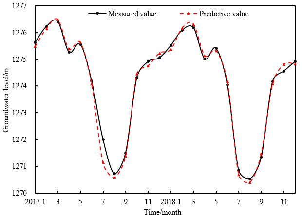
Water 2019, 11, 860                                                                                                10 of 20

indicated that the prediction accuracy of the ABC-BP model was high and met simulation accuracy
requirement. However, the AE values were maintained at approximately 0.46 in the optimal training
of the BP model, and serious AE errors that exceeded 1.1 occurred during individual training. This
result failed to meet the accuracy requirement for groundwater level prediction. The AE values of
the PSO-BP and GA-BP models in the optimal training were kept at approximately 0.28 and 0.35,
respectively. Although the predicted values were acceptable in most cases for the PSO-BP and GA-BP
models, the AE values of the two models were higher than those of the ABC-BP model. As a result,
the ABC-BP model comparatively performed best in the prediction effect of groundwater levels, and
the simulated values of groundwater levels were closest to the true values. PSO-BP ranked second,
followed   by GA-BP, and the BP model demonstrated the worst performance.
       Water 2019, 1, x                                                                11 of 23

       Figure 6. Variation curve of MSE in the optimal and worst training of the ABC-BP and BP models.
            Figure 6. Variation curve of MSE in the optimal and worst training of the ABC-BP and BP
            models.
     In addition to AE and RE, four error representations were used to compare several algorithms
to better illustrate   the the
              In addition,  filtering   effects
                                predicted        of the
                                           and error     fourofmodels
                                                      values             andmodel
                                                                the ABC-BP    highlight    the superiority
                                                                                    were compared              of the
                                                                                                      with those   of ABC
algorithm.   The coefficient     of determination        2
       the PSO-BP,    GA-BP, and    BP models under(Rthe) represents     the degree
                                                            optimal training          of relevant
                                                                              conditions            correlation
                                                                                          in this work.             between
                                                                                                          The fitting
the measured      and predicted     values.   The  closer  R 2 is to “1”, the higher the correlation is. Conversely,
       results of groundwater levels in the monitoring well ZB-03, as shown in Table 2 and Figure 7, were
the closer R2 is to “0”, the lower the correlation is [45]. As listed in Table 3, the R2 values of the ABC-BP,
       used as examples. All the absolute error (AE) values remained within 0.16 when the network
PSO-BP, GA-BP, and BP models were 0.983, 0.864, 0.826, and 0.653, respectively. It illustrated that
       training of the ABC-BP model ran optimally, and the change range of AE and RE were minimal.
the ABC-BP model matched better than the other three models. Moreover, the other three errors of
       Such results indicated that the prediction accuracy of the ABC-BP model was high and met
the ABC-BP model were smaller than those of the three other models. The root MSE (RMSE) and
       simulation accuracy requirement. However, the AE values were maintained at approximately 0.46
maximum RE (REmax) of the PSO algorithm were smaller than those of the GA algorithm, whereas
       in the optimal training of the BP model, and serious AE errors that exceeded 1.1 occurred during
their mean AE (MAE) were similar. The RMSE, MAE, and REmax of the BP model were the highest,
       individual training. This result failed to meet the accuracy requirement for groundwater level
thereby indicating that the traditional BP neural network provided the worst prediction accuracy. The
       prediction. The AE values of the PSO-BP and GA-BP models in the optimal training were kept at
comparative analysis results of the four models were found that the ABC-BP model exhibited the better
       approximately 0.28 and 0.35, respectively. Although the predicted values were acceptable in most
prediction  accuracy and optimization performance, followed by the PSO-BP, GA-BP, and BP models in
       cases the
turn. Thus,   for the
                   ABCPSO-BP    and GA-BP
                         algorithm           models, to
                                      was selected     theoptimize
                                                           AE valuesthe
                                                                      of the
                                                                          BP two models
                                                                             neural        were higher
                                                                                     network              thansimulate
                                                                                                 to further    those    the
       of  the  ABC-BP     model.   As  a  result, the  ABC-BP
groundwater levels of the six wells in the next part of this work.model   comparatively    performed    best  in  the
       prediction to
     According      effect of groundwater
                       Figure                  levels, values
                                 8, the measured       and theofsimulated   valueswere
                                                                   the six wells    of groundwater      levels phase
                                                                                          in the recovery       were from
       closest   to the  true   values.  PSO-BP    ranked   second,  followed   by  GA-BP,    and
January 2017 to March 2017, October 2017 to March 2018, and October 2018 to December 2018 which     the   BP  model
was in demonstrated    the worst
        the non-irrigation         performance.
                                period    when minimal mining activities were conducted. As summer and
autumn irrigation began, exploitation amount dramatically increased, and thus, groundwater level
             Table 2. Comparison results of groundwater level prediction obtained using the ABC-BP,
gradually dropped from April 2017 to September 2017 and April 2018 to September 2018. The predicted
             PSO-BP, GA-BP, and BP models.
values of the six monitoring wells obtained using the ABC-BP model fitted the measured values well.
      Test Sample           ABC-BP Model            PSO-BP Model             GA-BP Model                BP Model
            Measured     Predictive   Absolute   Predictive   Absolute    Predictive   Absolute   Predictive   Absolute
  Month        Value       Value       Error       Value        Error       Value       Error       Value        Error
                (m)         (m)                     (m)                      (m)                      (m)
  2017/1      1280.24     1280.29       0.05      1280.43       0.19       1280.76       0.52       1279.55      −0.69
Water 2019, 11, 860 11 of 20
Water 2019, 1, x 12 of 23
This result further illustrated that the ABC-BP model can effectively express the nonlinear relationship
2017/3 the
between 1280.55 1280.63
four aforementioned 0.08 1280.71
influencing 0.16 groundwater
factors and 1281.16 level.
0.61The ABC-BP
1281.65 model1.10can
also accurately
2017/4 simulate
1279.91 the trend
1279.82 of groundwater
−0.09 1279.54 levels.
−0.37In summary,
1280.14 the ABC-BP
0.23 model
1279.02 can be used
−0.89
as an
2017/5effective tool
1280.02 for forecasting
1279.96 the
−0.06 future groundwater
1280.56 0.54 levels of Yaoba
1279.63 Oasis.
−0.39 1280.21 0.19
2017/6 1279.25 1279.18 −0.07 1279.42 0.17 1278.69 −0.56 1280.11 0.86
Table 2. Comparison results of groundwater level prediction obtained using the ABC-BP, PSO-BP,
2017/7 1278.61 1278.50 −0.11 1278.20 −0.41 1278.74 0.13 1279.27 0.66
GA-BP, and BP models.
2017/8 1279.03 1278.99 −0.04 1278.82 −0.21 1279.46 0.43 1279.26 0.23
2017/9 Test1279.14
Sample ABC-BP Model
1279.21 0.07 PSO-BP Model
1279.32 0.18 GA-BP Model0.29
1279.43 BP Model
1278.72 −0.42
Measured Predictive Predictive Predictive Predictive
2017/10
Month 1279.59
Value 1279.56
Value −0.03
Absolute 1279.34
Value −0.25
Absolute 1280.22
Value 0.63
Absolute 1279.46 Absolute
Value −0.13
Error Error Error Error
2017/11 1280.06
(m) 1280.19
(m) 0.13 1279.74
(m) −0.32 1280.55
(m) 0.49 1280.64
(m) 0.58
2017/1 1280.24 1280.29 0.05 1280.43 0.19 1280.76 0.52 1279.55 −0.69
2017/12
2017/2
1280.27
1280.49
1280.22
1280.60
−0.05
0.11
1280.55
1280.95
0.28
0.46
1280.11
1280.22
−0.16
−0.27
1280.38
1280.83
0.11
0.34
2018/1
2017/3 1279.64
1280.55 1279.52
1280.63 −0.12
0.08 1279.95
1280.71 0.31
0.16 1280.21
1281.16 0.57
0.61 1279.98
1281.65 0.34
1.10
2017/4 1279.91 1279.82 −0.09 1279.54 −0.37 1280.14 0.23 1279.02 −0.89
2018/2
2017/5 1279.81
1280.02 1279.73
1279.96 −0.08
−0.06 1280.28
1280.56 0.47
0.54 1280.09
1279.63 0.28
−0.39 1279.66
1280.21 −0.15
0.19
2017/6 1279.25 1279.18 −0.07 1279.42 0.17 1278.69 −0.56 1280.11 0.86
2018/3 1279.92 1279.86 −0.06 1280.05 0.13 1279.81 −0.11 1280.29 0.37
2017/7 1278.61 1278.50 −0.11 1278.20 −0.41 1278.74 0.13 1279.27 0.66
2018/4
2017/8 1279.16
1279.03 1279.27
1278.99 0.11
−0.04 1279.25
1278.82 0.09
−0.21 1279.69
1279.46 0.53
0.43 1279.60
1279.26 0.230.44
2017/9 1279.14 1279.21 0.07 1279.32 0.18 1279.43 0.29 1278.72 −0.42
2018/5
2017/10 1279.44
1279.59 1279.51
1279.56 0.07
−0.03 1278.93
1279.34 −0.51
−0.25 1279.55
1280.22 0.11
0.63 1279.21
1279.46 −0.23
−0.13
2017/11
2018/6 1280.06
1278.48 1280.19
1278.64 0.13
0.16 1279.74
1278.74 −0.32
0.26 1280.55
1278.80 0.49
0.32 1280.64
1277.57 0.58
−0.91
2017/12 1280.27 1280.22 −0.05 1280.55 0.28 1280.11 −0.16 1280.38 0.11
2018/7
2018/1 1278.12
1279.64 1278.03
1279.52 −0.09
−0.12 1278.47
1279.95 0.35
0.31 1277.76
1280.21 −0.36
0.57 1278.65
1279.98 0.53
0.34
2018/2 1279.81 1279.73 −0.08 1280.28 0.47 1280.09 0.28 1279.66 −0.15
2018/8
2018/3 1278.26
1279.92 1278.38
1279.86 0.12
−0.06 1278.15
1280.05 −0.11
0.13 1277.81
1279.81 −0.45
−0.11 1278.51
1280.29 0.25
0.37
2018/9
2018/4 1278.42
1279.16 1278.34
1279.27 −0.08
0.11 1278.72
1279.25 0.30
0.09 1278.52
1279.69 0.10
0.53 1279.03
1279.60 0.61
0.44
2018/5 1279.44 1279.51 0.07 1278.93 −0.51 1279.55 0.11 1279.21 −0.23
2018/10
2018/6 1278.79
1278.48 1278.85
1278.64 0.06
0.16 1278.64
1278.74 −0.15
0.26 1279.25
1278.80 0.46
0.32 1278.48
1277.57 −0.31
−0.91
2018/7 1278.12 1278.03 −0.09 1278.47 0.35 1277.76 −0.36 1278.65 0.53
2018/11
2018/8
1279.31
1278.26
1279.23
1278.38
−0.08
0.12
1279.55
1278.15
0.24
−0.11
1279.57
1277.81
0.26
−0.45
1279.57
1278.51
0.26
0.25
2018/12
2018/9 1279.56
1278.42 1279.42
1278.34 −0.14
−0.08 1279.99
1278.72 0.43
0.30 1279.73
1278.52 0.17
0.10 1279.99
1279.03 0.43
0.61
2018/10 1278.79 1278.85 0.06 1278.64 −0.15 1279.25 0.46 1278.48 −0.31
2018/11 1279.31 1279.23 −0.08 1279.55 0.24 1279.57 0.26 1279.57 0.26
2018/12 1279.56 1279.42 −0.14 1279.99 0.43 1279.73 0.17 1279.99 0.43
Figure 7. Fitting curve of the measured and predicted values obtained using the ABC-BP, PSO-BP,
GA-BP, and BP models.Water 2019, 11, 860 12 of 20
Table 3. Comparison of four error representations of the ABC-BP, PSO-BP, GA-BP, and BP models.
Error Name of Models
Representations ABC-BP PSO-BP GA-BP BP
R2 0.983 0.864 0.826 0.653
RMSE 0.092 0.316 0.390 0.533
MAE 0.086 0.288 0.352 0.460
REmax 0.013 0.043 0.049 0.086
Water 2019, 1, x 14 of 23
(a) ZB-01 well
(b) ZB-02 well
Figure 8. Cont.Water 2019, 11, 860 13 of 20
Water 2019, 1, x 15 of 23
(c) ZB-03 well
(d) ZB-04 well
Figure 8. Cont.Water 2019, 11, 860 14 of 20
Water 2019, 1, x 16 of 23
(e) ZB-05 well
(f) ZB-06 well
Figure Figure 8. curve
8. Fitting Fittingofcurve of the measured
the measured and predicted
and predicted values of values of six monitoring
six monitoring wellsusing
wells obtained
obtained using the ABC-BP model.
the ABC-BP model.
3.2. Groundwater
3.2. Groundwater LevelLevel Prediction
Prediction under
under thethe ExistingMining
Existing Mining Scenario
Scenario
In this study, the trained ABC-BP model with double hidden layers was applied to predict the
In this study, the trained ABC-BP model with double hidden layers was applied to predict the
monthly groundwater levels of six monitoring wells. The prediction results of the six wells from
monthly groundwater levels of six monitoring wells. The prediction results of the six wells from 2019 to
2019 to 2030 under the existing mining scenario are provided in Table 4 and Figure 9. As seen from
2030 under
Tablethe existing
4, the mining level
groundwater scenario are provided
of Yaoba in Table
Oasis under 4 and Figure
the exploitation of 9.
40As seen m
million from Table
3/year will4, the
rate/year
groundwater level 3
gradually dropofwith
Yaoba Oasis
a total under
range themexploitation
of 1.31 to 5.50 m andofa 40 million m
descending will gradually
of 0.11–0.46 m/a. The drop
with a total range of 1.31 m to 5.50 m and a descending rate of 0.11–0.46 m/a. The groundwater level
of ZB-03 will gradually drop from 1279.51 m in 2019 to 1274.01 m in 2030, which will be the largest
dropping occurring in the central and southern areas. The analysis result of the simulated values
shows that the decreased amplitude of groundwater level will be 0.71–1.68 m from 2019 to 2024 with aWater 2019, 11, 860 15 of 20
decline rate of 0.12–0.28 m/a. The decline of groundwater level from 2025 to 2030 will be 0.59–3.82 m,
and the drop speed will be 0.10–0.64 m/a. In summary, the cumulative decline range of groundwater
level from 2019 to 2030 will be large given the current mining mode.
Table 4. Analysis of variation for groundwater level from 2019 to 2030 different mining scenarios.
Variation Range of Groundwater Levels from 2019 to
Monitoring 2030 Under Different Mining Scenarios (m)
Water 2019, 1,Well
x Location 17 of 23
40 million m3 /year 31 million m3 /year 22 million m3 /year
groundwater
ZB-01 level of ZB-03 will gradually
North Central drop−1.31
from 1279.51 m in 2019 to 1274.01 m in 2030,
0.13 which
6.73
will ZB-02
be the largest dropping occurring in the central
Central −2.81 and southern areas.
0.01 The analysis result of the
7.24
simulated
ZB-03 values shows thatCentral
South the decreased amplitude
−5.50 of groundwater 0.04
level will be 0.71–1.685.86
m from
2019ZB-04
to 2024 with a decline
West rate of 0.12–0.28 m/a.−1.79
Central The decline of groundwater
0.07 level from 20258.47
to 2030
will ZB-05
be 0.59–3.82 m, and the drop speed will be−3.52
South 0.13 the cumulative6.64
0.10–0.64 m/a. In summary, decline
rangeZB-06
of groundwater levelSouth −2.61
from 2019 to 2030 will 0.22 mining mode. 6.11
be large given the current
Figure 9. Figure 9. Duration curves of groundwater levels in six monitoring wells from 2019 to 2030
Duration curves of groundwater levels in six monitoring wells from 2019 to 2030 under the
under the existing mining scenario.
existing mining scenario.
Figure 9 clearly illustrates that the six monitoring wells exhibited a gradual declining
Figure 9 clearly
tendency. The illustrates that
analysis of the thesituation
local six monitoring wells
indicated that exhibited
the amount a gradual exploitation
of groundwater declining tendency.
The analysis of the local situation indicated that the amount of groundwater exploitation
at present is maintained at approximately 40 million m /year, which already exceeds the total
3 at present is
maintained at approximately 40 million m /year, which already exceeds the total recharge amount of
recharge amount of 31 million m 3
3/year in the study area. Under the existing mining condition, the
31 millionexploitation
m3 /year inquantity
the studyis greater than the
area. Under thelocally allowed
existing mining mining level. Consequently,
condition, the exploitationthe quantity
groundwater levels will drop considerably in the future and may cause substantial damage to
is greatergroundwater
than the locally allowed mining level. Consequently, the groundwater levels will drop
circulation and the eco-environment. With the future development of the social
considerably in the
economy, futureand
industry, and may cause
agriculture, substantial
groundwater damage
demand to groundwater
can increase considerably.circulation
Hence, the and the
eco-environment. With
decline rate and the future
amplitude development
of groundwater of be
level will thelarger
social
thaneconomy,
the predictedindustry,
value. and agriculture,
groundwater demand can increase considerably. Hence, the decline rate and amplitude of groundwater
3.3. Groundwater Level Prediction under Different Mining Scenarios
level will be larger than the predicted value.
The amount of groundwater exploitation should be optimized to ensure the sustainable
utilization of groundwater
3.3. Groundwater Level Predictioninunder
the study area [53].
Different The ABC-BP
Mining model was trained by continuously
Scenarios
adjusting the input value of the exploitation amount and then to predict the groundwater levels of
The amount of groundwater
six monitoring exploitation
wells under different miningshould beThe
scenarios. optimized
predictiontoresults
ensure the sustainable
of groundwater levelsutilization
from 2019
of groundwater intothe
2030 are summarized
study in Table
area [53]. The 4 and Figure
ABC-BP model10.was
Under the actual
trained mining situationadjusting
by continuously (40 the
million m3/year), groundwater level will be in the decline stage from 2019 to 2030, given the largest
input value of the exploitation amount and then to predict the groundwater levels of
drop of 5.50 m. As the exploitation quantity was adjusted to 31 million m3/year, groundwater level
six monitoring
wells under different mining scenarios. The prediction results of groundwater levels from 2019 toWater 2019, 11, 860 16 of 20
2030 are summarized in Table 4 and Figure 10. Under the actual mining situation (40 million m3 /year),
groundwater level will be in the decline stage from 2019 to 2030, given the largest drop of 5.50 m.
As the exploitation quantity was adjusted to 31 million m3 /year, groundwater level only changed
slightly and remained at a relatively stable value. Thereafter, groundwater level will enter the stable
stage. As the exploitation quantity was adjusted to 22 million m3 /year, groundwater level entered the
recovery stage and gradually rose with a largest increase of 8.47 m and a rate of 0.71 m/a.
Water 2019, 1, x 19 of 23
(a) Groundwater levels under the exploitation of 31 million m3/year
(b) Groundwater levels under the exploitation of 22 million m3/year
Figure 10. Duration curves of the groundwater levels of six monitoring wells from 2019 to
Figure 10. Duration curves of the groundwater levels of six monitoring wells from 2019 to 2030 under
2030 under different mining scenarios.
different mining scenarios.Water 2019, 11, 860 17 of 20
As evident in Figure 10, the variation trends of groundwater levels in the six monitoring wells are
generally consistent under the same mining conditions. Groundwater level will gradually increase
as exploitation quantity decreases. The groundwater system will gradually reach equilibrium as
exploitation amount declines to 31 million m3 /year, which is equal to the total recharge amount
(Figure 10a). Therefore, an exploitation amount of 31 million m3 /year is a reasonable value under the
current conditions of the study area and can meet the requirements of the sustainable utilization of
groundwater and the development of agriculture. Groundwater level will gradually rise as exploitation
amount decreases to 22 million m3 /year, and the damaged hydrological ecosystem will recover
(Figure 10b). Nevertheless, an exploitation of 22 million m3 /year will not guarantee the development
of efficient local agriculture and economy. In conclusion, the most appropriate amount of groundwater
exploitation for sustainable development in Yaoba Oasis is 31 million m3 /year.
Feasible solutions such as strengthening the scientific management of water resources,
implementing water-saving measures, improving the utilization rates of water resources, and adjusting
crop planting structure, can effectively reduce the exploitation amount of groundwater. Subsequently,
the results can change the status quo of mining. In future agricultural planning, the depressurization
of groundwater exploitation is essential for balancing groundwater mining, replenishing groundwater
resources, and achieving sustainable development for the agriculture, economy, and eco-environment
of Yaoba Oasis.
4. Conclusions
An ABC-BP model with double hidden layers was proposed to simulate and predict the
groundwater levels in Yaoba Oasis. The groundwater level data of six monitoring wells from
January 2010 to December 2016 and January 2017 to December 2018 were used as training and test
samples of the neural network, respectively. The data of the four major influencing factors, namely,
recharge, exploitation, rainfall, and evaporation, obtained from January 2010 to December 2016, were
used as input data. As constructed using a stepwise growing method and multi-trial algorithms,
the topology structure of the ABC-BP model with double hidden layers was 4-7-3-1, which could
overcome the over-fitting problem. The performance of the prediction model was determined by
training and testing the ABC-BP and BP models on the sample data, respectively. The comparative
analysis showed that the RE and MSE values in the optimal and worst training of the ABC-BP model
were lower than the results in the optimal training of the BP model. In addition, the ABC-BP model
obtained more consistent results and smaller MSE values after several training, compared with the BP
model. Moreover, the ABC-BP model presented more accurate prediction results, the highest R2 , and
smaller MAE, REmax, and RMSE values than the PSO-BP, GA-BP, and BP models. In summary, the
accuracy, convergence rate, and stabilization of the BP neural network with double hidden layers were
considerably improved by the ABC algorithm by overcoming the low accuracy and slow convergence
problems. Accordingly, the simulated values from January 2017 to December 2018 well fitted the
measured values of the six monitoring wells during the training process of the proposed ABC-BP model.
The trained ABC-BP model with double hidden layers was applied to predict the groundwater
levels in Yaoba Oasis from 2019 to 2030 under different mining scenarios. According to the prediction
results, the groundwater levels will rise gradually as exploitation quantity decreases. Groundwater
levels will enter the decline stage with a total decline range of 1.31 m to 5.50 m under the existing
mining scenario (40 million m3 /year), the stable stage with an exploitation amount of 31 million
m3 /year, and the recovery stage with an exploitation amount of 22 million m3 /year. Therefore, the
exploitation quantity of 31 million m3 /year was found to be applicable for the sustainable development
of groundwater resources in the study area.
The prediction of groundwater levels using the ABC-BP model in a typical oasis in the arid
northwest region of China was realized in this study. The research results can guide the scientific
utilization of groundwater and provide a novel approach for similar research in other arid oases with
the same characteristics. Further investigation is suggested to forecast the daily groundwater levelYou can also read