GS-WGAN: A Gradient-Sanitized Approach for Learning Differentially Private Generators
←
→
Page content transcription
If your browser does not render page correctly, please read the page content below
GS-WGAN: A Gradient-Sanitized Approach for
                                                   Learning Differentially Private Generators

                                                     Dingfan Chen1            Tribhuvanesh Orekondy2            Mario Fritz1
                                             1                                                  2
                                                 CISPA Helmholtz Center for Information Security Max Planck Institute for Informatics
                                                                      Saarland Informatics Campus, Germany
arXiv:2006.08265v1 [cs.LG] 15 Jun 2020

                                                                                        Abstract
                                                    The wide-spread availability of rich data has fueled the growth of machine learning
                                                    applications in numerous domains. However, growth in domains with highly-
                                                    sensitive data (e.g., medical) is largely hindered as the private nature of data
                                                    prohibits it from being shared. To this end, we propose Gradient-sanitized Wasser-
                                                    stein Generative Adversarial Networks (GS-WGAN), which allows releasing a
                                                    sanitized form of the sensitive data with rigorous privacy guarantees. In contrast to
                                                    prior work, our approach is able to distort gradient information more precisely, and
                                                    thereby enabling training deeper models which generate more informative samples.
                                                    Moreover, our formulation naturally allows for training GANs in both centralized
                                                    and federated (i.e., decentralized) data scenarios. Through extensive experiments,
                                                    we find our approach consistently outperforms state-of-the-art approaches across
                                                    multiple metrics (e.g., sample quality) and datasets.

                                         1   Introduction
                                         Releasing statistical and sensory data to a broad community has contributed towards advances in
                                         numerous machine learning (ML) techniques e.g., object recognition (ImageNet [10]), language
                                         modeling (RCV [22]), recommendation systems (Netflix ratings [6]). However, in many sensitive
                                         domains (e.g., medical, financial), similar advances are often held back as the private nature of
                                         collected data prohibits release in its original form. Privacy-preserving data publishing [5, 12, 15]
                                         provides a reasonable solution, where only a sanitized form of the original data (with rigorous privacy
                                         guarantees) is publicly released.
                                         Traditionally, sanitization is performed in a differentially private (DP) framework [11]. The saniti-
                                         zation method employed is often hand-crafted for the given input data [26, 28, 42] and the specific
                                         data-dependent task the sanitized data is intended for (e.g., answering linear queries) [7, 13, 19, 34].
                                         As a result, such sanitization techniques greatly restrict the expressiveness of the released data
                                         distribution and fail to generalize to novel tasks unanticipated by the publisher. Instead, recent
                                         privacy-preserving techniques [5, 40, 41, 43] build on top of successes in generative adversarial
                                         network (GANs) [16] literature, to generate synthetic data faithful to the original input distribution.
                                         Specifically, GANs are trained using a privacy-preserving algorithm (e.g., using DP-SGD [1]) and
                                         demonstrate promising results in modeling a variety of real-world high-dimensional data distributions.
                                         Common to most privacy-preserving training algorithms for neural network models is manipulating
                                         the gradient information generated during backpropagation. Manipulation most commonly involves
                                         clipping the gradients (to bound sensitivity) and adding calibrated random noise (to introduce stochas-
                                         ticity). Although recent techniques that employ such an approach demonstrate reasonable success,
                                         they are largely limited to shallow networks and fail to sufficiently capture the sample quality of the
                                         original data.
                                         In this paper, towards the goal of a generative model capable of synthesizing high-quality samples
                                         in a privacy-preserving manner, we propose a differentially private GAN. We first identify that in

                                         Preprint. Under review.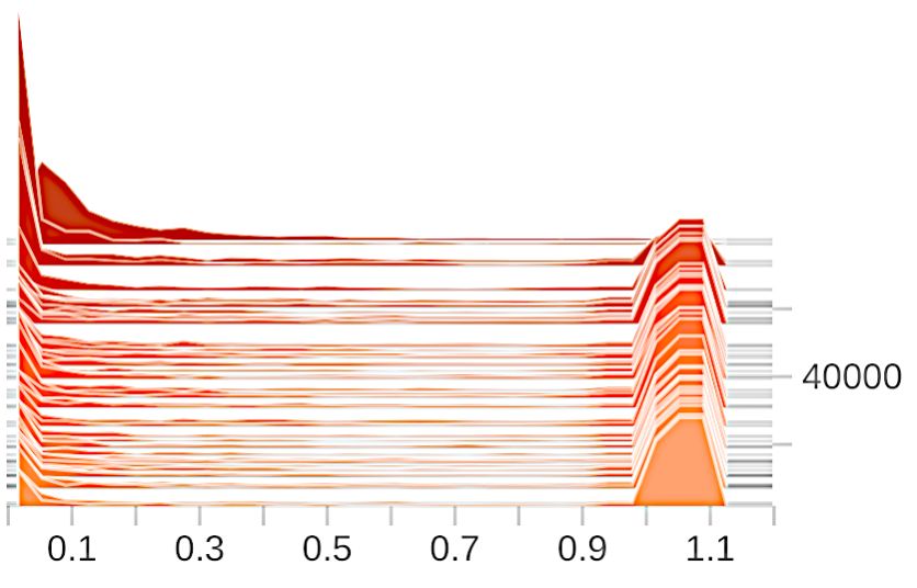
such a data-publishing scenario, only a subset of the trained model (specifically the generator) and its
parameters need to be publicly-released. This insight allows us to surgically manipulate the gradient
information during training, and thereby allowing more meaningful gradient updates. By coupling
the approach with a Wasserstein [2] objective with gradient-penalty term [17], we further improve
the amount of gradient information flow during training. The new objective additionally allows us
to precisely estimate the gradient norms and analytically determine the sensitivity values. As an
added benefit, we find our approach bypasses an intensive and fragile hyper-parameter search for
DP-specific hyperparameters (particularly clipping values).
Contributions. (i) A novel gradient-sanitized Wasserstein GAN (GS-WGAN), which is capable
of generating high-dimensional data with DP guarantee; (ii) Our approach naturally extends to both
centralized and decentralized datasets. In the case of decentralized scenarios, our work can provide
user-level DP guarantee [24] under an untrusted server; (iii) Extensive evaluations on various datasets
demonstrate that our method significantly improves the sample quality of privacy-preserving data
over state-of-the-art approaches.

2   Related Work
We review several generative models in the area of differential privacy, as well as their relations to
our work.
DP-SGD GAN. Training GANs via DP-SGD [1, 5, 36, 40, 43] has proven effective in generating
high-dimensional sanitized data. However, DP-SGD relies on carefully tuning of the clipping bound
of gradient norm, i.e., the sensitivity value. Specifically, the optimal clipping bound varies greatly with
the model architecture and the training dynamics, making the implementation of DP-SGD difficult.
Unlike DP-SGD, our framework provides precise estimation of the sensitivity value, avoiding the
intensive search of hyper-parameters.
PATE. Private Aggregation of Teacher Ensembles (PATE) is recently adapted to generative models
and two main approaches were studied: PATE-GAN [41] and G-PATE [27]. PATE-GAN trained
multiple teacher discriminators on disjoint data partitions together with a student discriminator. In
contrast, we consider a simplified model without a student discriminator.
G-PATE [27] is similar to our work in the sense that, both works trained the discriminator non-
privately while only training the generator with DP guarantee, and both sanitized gradients that the
generator received from the discriminator. However, G-PATE suffers from two main limitations:
(i) gradients need to be discretized by using manually selected bins in order to suit for the PATE
framework and (ii) high-dimensional gradients in the PATE framework bring high privacy costs and
thus dimension reduction techniques are required. Our framework can effectively avoid these two
limitations and achieve better sample quality due to the novel gradient sanitation, see our experiments.
Fed-Avg GAN [3]. While many works focus on centralized setting, the decentralized case has
rarely been studied. To address this, Federated Average GAN (Fed-Avg GAN) proposed to adapt
GAN training by using the DP-Fed-Avg [29] algorithm, providing user-level DP guarantee under
trusted server. In comparison with Fed-Avg GAN that merely works on decentralized data, our work
can tackle both centralized and decentralized data using a single framework. Note that Fed-Avg
sanitized parameter gradients of the discriminator in a similar way to DP-SGD, it also suffers from
the difficulty of turning hyper-parameters.

3   Background
DP provides rigorous privacy guarantees for algorithms while allowing for quantitative privacy
analysis. We below present several definitions and theorems that will be used in this work.
Definition 3.1. (Differential Privacy (DP) [11]) A randomized mechanism M with range R is
(ε, δ)-DP, if
                           P r[M(S) ∈ O] ≤ eε · P r[M(S 0 ) ∈ O] + δ                        (1)
holds for any subset of outputs O ⊆ R and for any adjacent datasets S and S 0 , where S and S 0 differ
from each other with only one training example. M is the GAN training algorithm in our case, ε
corresponds to the upper bound of privacy loss, and δ is the probability of breaching DP constraints.

                                                    2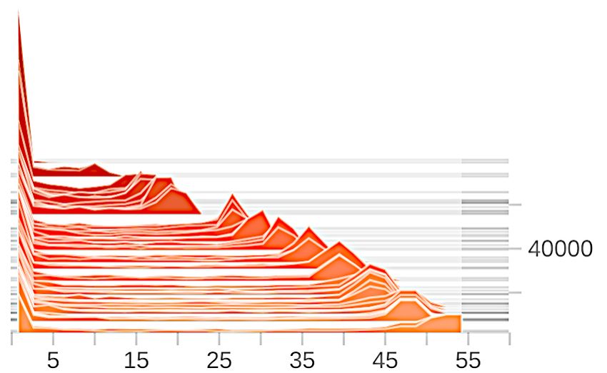
Definition 3.2. (Rényi Differential Privacy (RDP) [31]) A randomized mechanism M is (λ, ε)-RDP
with order λ, if
                                                        "                  λ−1 #
                             0        1                     P r[M(S) = x]
           Dλ (M(S)kM(S )) =              log Ex∼M(S)                              ≤ε       (2)
                                    λ−1                    P r[M(S 0 ) = x]

holds for any adjacent datasets S and S 0 , where Dλ (P kQ) =              1
                                                                          λ−1     log Ex∼Q [(P (x)/Q(x))λ ] denotes
                                                                                           log 1/δ
the Rényi divergence. Moreover, a (λ, ε)-RDP mechanism M is also (ε +                        λ−1 , δ)-DP.

In contrast to DP, RDP provides convenient composition properties to accumulate privacy cost over a
sequence of mechanisms.
Theorem 3.1. (Composition) For a sequenceP of mechanisms M1 , ..., Mk s.t. Mi is (λ, εi )-RDP
∀i, the composition M1 ◦ ... ◦ Mk is (λ, i εi )-RDP.
Definition 3.3. (Gaussian Mechanism [14, 31]) Let f : X → Rd be an arbitrary d-dimensional
function with sensitivity being
                                                ∆2 f = max0 kf (S) − f (S 0 )k2                                  (3)
                                                        S,S

over all adjacent datasets S and S 0 . The Gaussian Mechanism Mσ , parameterized by σ, adds noise
into the output,i.e.,
                                     Mσ (x) = f (x) + N (0, σ 2 I).                           (4)
                   2
M is (λ, λ∆ 2f
           2σ 2 )-RDP.
Theorem 3.2. (Post-processing [14]) If M satisfies (ε, δ)-DP, F ◦ M will satisfy (ε, δ)-DP for any
function F with ◦ denoting the composition operator.

4   Proposed Method
Generative Adversarial Networks (GANs) [16]. Our approach models the underlying (private)
data distribution using a generative neural network, building on top of recent successes of GANs.
GANs (see Fig. 1(a)) formulate the task of sample generation as a zero-sum two-player game, between
two neural network models: discriminator D and generator G. The discriminator D is rewarded for
correctly classifying whether a given sample is ‘real’ (i.e., from the input data distribution) or ‘fake’
(generated by the generator). In contrast, the task of the generator G is (given some random noise z)
to generate samples which fool the discriminator (i.e., causes misclassifications). After training the
models in an adversarial manner, the discriminator is discarded and the generator is used as a proxy
to draw samples from the original distribution.
Differentially Private GANs. Releasing the generator as a substitute for the original training data
distribution entails privacy risks. Consequently, along the lines of recent work [5, 36, 40, 43], our
goal is instead to train the GAN in a privacy-preserving manner, such that any privacy leakage upon
disclosing the generator is bounded. A simple approach towards the goal is replacing the typical
training procedure (SGD) with a differentially private variant (DP-SGD [1]) and thereby limiting
the contribution of a particular training example in the final trained model. DP-SGD enforces the
desired privacy requirement by (i) clipping the gradients gt to have an L2 -norm of C at each training
step; and (ii) sampling random noise and adding it to the gradients, before performing descent on the
trained parameters θ:
           g (t) := ∇θ L(θD , θG )                                                                 (gradient)    (5)
           ĝ (t) := Mσ,C (g (t) ) = clip(g (t) , C) + N (0, σ 2 C 2 I)             (sanitization mechanism)     (6)
          (t+1)          (t)              (t)
      θ           := θ         − η · ĝ                                                (gradient descent step)   (7)

While such an approach provides rigorous privacy guarantees, there are multiple shortcomings: (i)
the sanitization mechanism Mσ,C , primarily due to clipping, significantly destroys the original
gradient information, and thereby affects utility; and (ii) finding a reasonable clipping value C
in the mechanism to balance utility with privacy is especially challenging. In particular, as the
gradient norms exhibit a heavy-tailed distribution, choosing a clipping value requires an exhaustive

                                                              3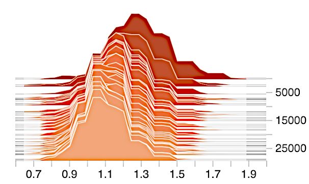
θG                         θD                         θG                            θD                           θG

                                                                                                                                                  …

                                                                                                                                                  …
                                                                       gradient                                                  gradient
                                                                     sanitization                                              sanitization
                                       sensitive                                                sensitive
                                         data                                                     data
     non-private   sensitive         (ε,δ)-private   accessible by                  not accessible by          accessible by                  not accessible by
                                                       adversary                        adversary                adversary                        adversary

(a) Vanilla GAN                                      (b) GS-WGAN                                              (c) Fed-GS-WGAN
(Without privacy barrier)                            (Ours, with privacy barrier)                             (Ours, in a Federated setup)

Figure 1: Approach outline. Our gradient sanitization scheme ensures DP training of the generator.
search. Moreover, since the clipping value is extremely sensitive to many other hyperparameters (e.g.,
learning rate, architecture), it requires persistent re-tuning. Now, we discuss how we address these
shortcomings within our differentially private GAN approach.
Selectively applying Sanitization Mechanism. We begin by exploiting the fact that after training
the GAN, only the generator G is released. Consequently, we can perform gradient steps by selectively
applying the sanitization mechanism only to the corresponding subset of parameters θG :
                    (t+1)                 (t)           (t)                                             (t)   (t)
                   θD           := θD − ηD · gD                                                 (ĝD = gD ; Discriminator)                                         (8)
                    (t+1)                 (t)           (t)                                  (t)                    (t)
              θG    := θG − ηG · ĝG                 (ĝG = Mσ,C (gG ); Generator)                (9)
Apart from reducing the number of parameters sanitized, this also provides a benefit of more reliably
training a discriminator. In addition, we exploit the chain rule to further narrow the scope of the
sanitization mechanism:

                                    gG = ∇θG LG (θG ) = ∇G(z;θG ) LG (θG ) · JθG G(z; θG )                                                                        (10)
                                    ĝG = Mσ,C (∇G(z) LG (θG )) · JθG G(z; θG )                                                                                   (11)
                                                |    {z     } |        {z    }
                                                                upstream                         local
                                                                                                JG
                                                               gG

The above becomes easier to intuit by considering a typical loss function LG (θG ) = −D(G(z; θG )).
As illustrated in Fig. 1(b), Eq. 11 can then be considered as placing the privacy barrier for gradient
information backpropagating from the discriminator back to the generator, by applying the sanitization
                  upstream                               local
mechanism on gG            . Note that the second term (JG     ) is the local generator jacobian computed
independent of training data, and hence does not require sanitization. Consequently, using a more
precise application of the sanitization mechanism on the gradient information, our goal here is to
maximally preserve the true gradient direction during training.
Bounding sensitivity using Wasserstein distance. To bound the sensitivity of the optimizer on
individual training examples, a key step in sanitization mechanisms is to clip (Eq. 6) the gradient
vector g (Eq. 5) before updating parameters (Eq. 7). Clipping is typically performed in L2 norm,
by replacing the gradient vector g by g/max(1, ||g||2 /C) to ensure ||g||2 ≤ C. However, clipping
significantly destroys gradient information, as reasonable choices of C (e.g., 4 [1]) are significantly
lower than the gradient-norms observed (12 ± 10 in our case) when training neural networks
using standard loss functions. We propose to alleviate the issue by leveraging a more suitable loss
function, which generates bounded gradients (with norms close to 1) by construction. Specifically,
we use as our loss the Wasserstein-1 metric [2], which measures the statistical distance between the
real and generated data distributions. Here, theR training Rprocess can be interpreted as minimizing
integral probability metrics (IPMs) supf ∈F | M f dP − M f dQ| between real (P ) and generated
(Q) data distributions, where F = {f : kf kL ≤ 1} (i.e., the discriminator function f is 1-Lipschitz
continuous). It follows that the optimal discriminator has a gradient norm being 1 almost everywhere
under P and Q.
We incorporate the norm constraint into our training objective in the form of a gradient penalty term
[17]:

                                                                                                                                                   2
               LD = −Ex∼P [D(x)] + Ex̃∼Q [D(x̃)] + λE[(k∇D(αx + (1 − α)x̃)k2 − 1) ]                                                                               (12)
               LG = −Ez∼Pz [D(G(z))]                                                                                                                              (13)

                                                                                4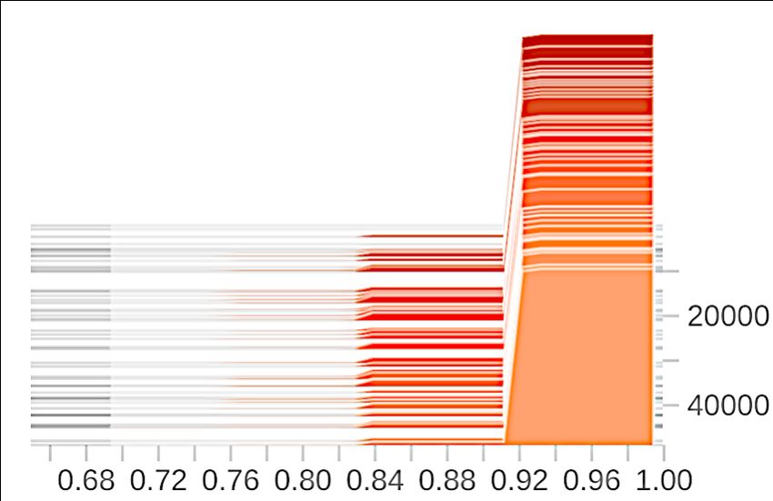
weight (1. layer)                                                1.6

                                                                                                             average gradient norm
                                                    250.0           weight (2. layer)

                            average gradient norm
                                                                                                                                     1.5
                                                    200.0           bias (1. layer)
                                                                                                                                     1.4
                                                    150.0           bias (2. layer)
                                                                                                                                     1.3
                                                    100.0
                                                                                                                                     1.2
                                                     50.0
                                                                                                                                     1.1
                                                      0.0
                                                            0   10k 20k 30k 40k 50k 60k 70k                                                0   10k 20k 30k 40k 50k 60k 70k 80k
                                                                         iterations                                                                      iterations

       (a) DP-SGD                                               (b) DP-SGD                        (c) Ours                                         (d) Ours
Figure 2: Gradient norm (before clipping) dynamics during the GAN training process. In the
experiment, the clipping bound is chosen to be 1 and 1.1 in 2(c) and 2(a) respectively.
where LD and LG represent training objectives for the discriminator and the generator, respectively.
λ is the hyper-parameter for weighting the gradient penalty term and Pz denotes the prior distribution
for the latent code variable z. The variable α ∼ U[0, 1], uniformly sampled from [0, 1], regulates the
interpolation between real and generated samples.
As a natural consequence of the Wasserstein objective, reducing the norms of our target gradient
  upstream
gG         ( Equation 11) during training is integrated in our training objective (last term in Equation 12).
Consequently, we observe significantly lower gradient norms during training (see Fig. 2(c)-2(d))
compared to training using a standard GAN loss (see Fig. 2(a)-2(b)). As a result, bounding the
sensitivity (i.e., gradient norms) is now largely delegated to our training procedure and clipping
using the sanitization mechanism destroys significantly less information. Additionally, by choosing a
clipping threshold of C=1 (i.e., ||g||2 ≤ 1), we obtain a fixed and bounded sensitivity, and eliminate
the need for intensive hyper-parameter search for the optimal clipping threshold. Following this
normalization solution, a data-independent privacy cost can be determined by the following theorem,
whose proof is provided in Appendix.
Theorem 4.1. Each generator update step satisfies (λ, 2Bλ/σ 2 )-RDP where B is the batch size.
Privacy Amplification by Subsampling. A well-known approach for increasing privacy of a
mechanism is to apply the mechanism to a random subsample of the database, rather than on the
entire dataset [4, 25, 38]. Intuitively, subsampling decreases the chances of leaking information about
a particular individual since nothing about that individual can be leaked once the individual is not
included in the subsample. In order to further reduce the privacy cost, we subsample the whole
dataset into different subsets and train multiple discriminators independently on each subset. At
each training step, the generator randomly queries one discriminator while the selected discriminator
updates its parameters on the generated data and its associated subsampled dataset.
Extending to Federated Learning. In addition to improving the privacy guarantee, performing
subsampling in our setup also naturally accommodates training a generative model on decentralized
datasets (with a discriminator trained on each disjoint data subset). Recently, Augenstein et al. [3]
identified such techniques are extremely relevant when training models in a federated setup [30],
i.e., when the training data is private and distributed among edge devices. We outline our method
to train a differentially private GAN in a federated setup in Figure 1(c) and remark some subtle
differences between our approach and Fed-Avg GAN [3] here: (i) the discriminators are retained at
each client in our framework while they are shared between the server and client in Fed-Avg GAN;
(ii) the gradients are sanitized at each client before sending to the server, with which we provide DP
guarantee even under an untrusted server. In contrast, the unprocessed information is accumulated
at the server before being sanitized in Fed-Avg GAN; and (iii) The gradients w.r.t. the samples are
transferred in GS-WGAN, while Fed-Avg GAN transfers the gradients w.r.t. discriminator network
parameters.

5     Experiment
5.1   Experiment Setup

To validate the applicability of our method to high-dimensional data, we conduct experiments on
image datasets. In line with previous works, we use MNIST [21] and Fashion-MNIST [39] dataset.
We model the joint distribution of images and the corresponding labels, i.e., the label is supplied
to both the generator and the discriminator, and the image is generated conditioned on the input.
During both training and inference, we use a uniform prior distribution for generating labels, which

                                                                                              5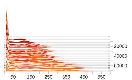
IS↑     FID ↓    MLP ↑      CNN ↑      Avg ↑    Calibrated ↑
                                                             Acc        Acc        Acc         Acc
    MNIST              Real               9.80     1.02       0.98      0.99      0.88        100 %
                       G-PATE 1           3.85    177.16      0.25      0.51      0.34         40%
                       DP-SGD GAN         4.76    179.16      0.60      0.63      0.52         59%
                       DP-Merf            2.91    247.53      0.63      0.63      0.57         66%
                       DP-Merf AE         3.06    161.11      0.54      0.68      0.42         47%
                       Ours               9.23     61.34      0.79      0.80      0.60         69%
                       Real               8.98     1.49       0.88      0.91      0.79        100%
                       G-PATE             3.35    205.78      0.30      0.50      0.40         54%
    Fashion-MNIST      DP-SGD GAN         3.55    243.80      0.50      0.46      0.43         53%
                       DP-Merf            2.32    267.78      0.56      0.62      0.51         65%
                       DP-Merf AE         3.68    213.59      0.56      0.62      0.45         55%
                       Ours               5.32    131.34      0.65      0.65      0.53         67%
          Table 1: Quantitative Results on MNIST and Fashion-MNIST (ε = 10, δ = 10−5 )

is independent of the training dataset and thus does not incur additional privacy cost (in contrast, [36]
needs to assume the labels are non-private).
Evaluation Metrics. We evaluate along two fronts: privacy (determined by ε) and utility. For
utility, we consider two metrics: (a) sample quality: realism of the samples produced – evaluated
by Inception Score (IS) [23, 35] and Frechet Inception Distance (FID) [20] (standard in GAN
literature); and (b) usefulness for downstream tasks: we train downstream classifiers on 60k privately-
generated data points and evaluate the prediction accuracy on real test set. We consider Multi-layer
Perceptrons (MLP), Convolutional Neural Networks (CNN) and 11 scikit-learn [32] classifiers (e.g.,
SVMs, Random Forest). We include the following metrics in the main paper: MLP Acc (MLP
accuracy), CNN Acc (CNN accuracy), Avg Acc (Averaged accuracy of all classification models),
Calibrated Acc (Averaged accuracy of all classification models normalized by the accuracy when
trained on real data). The detailed results are presented in Appendix.
Architecture and Warm-start. We highlight two strategies adopted for improving the sample
quality as well as reducing the privacy cost: (i) Better model architecture: While previous works
are limited to shallow networks and thereby bottle-necking generated sample quality, our frame-
work allows stable training with a complex model architecture (DCGAN [33] architecture for the
discriminator, ResNet architecture (adapted from BigGAN [8]) for the generator) to help improve the
sample quality; and (ii) Discriminator warm-starting: To bootstrap the training process, we pre-train
discriminators along with a non-private generator for a few steps, and we subsequently train the
private generator by using the warm-starting values of the discriminators. Note that our framework
allows pre-training on the original private dataset without compromising privacy (in contrast, [43]
needs to use external public datasets).

5.2    Comparison with Baselines

Baselines. We consider the following state-of-the-art methods designed for DP high-dimensional
data generation: DP-Merf and DP-Merf AE [18], DP-SGD GAN [36, 40, 43], and G-PATE [27].
While PATE-GAN [41] demonstrates promising results on low-dimensional data, we currently do
not consider it as we were unable to extend it to our image datasets (more details in appendix) for
a fair comparison. For DP-Merf, DP-Merf AE, and G-PATE, we use the source code provided by
the authors. For DP-SGD GAN, we adopt the implementation of [36], which is the only work that
provides executable code with privacy analysis. For a fair comparison, we evaluate all methods
with a privacy budget of (ε, δ)=(10, 10−5 ) (consistently used in previous works) over 60K generated
samples.
Results. We present the qualitative results in Figure 3 and the quantitative results in Table 1. In
terms of sample quality, we find (Table 1, columns IS and FID) our method consistently provides
significant improvements over baselines. For instance, considering inception scores, we find a relative
improvement of 94% (9.23 vs. 4.76 of DP-SGD GAN) on MNIST and 45% on Fashion-MNIST
(5.32 vs. 3.68 of DP-Merf AE).
1
      PATE provides data-dependent ε, i.e., publishing ε value will introduce privacy cost. Thus, G-PATE is not
      directly comparable to other methods and is excluded from our analysis study (section 5.3).

                                                       6
Method MNIST Fashion-MNIST
G-PATE
DP-SGD GAN
DP-Merf
DP-Merf AE
Ours
Figure 3: Generated samples with (ε, δ) = (10, 10−5 )
10 10 10
DP-Merf DP-Merf
8 8 8 DP-Merf AE
DP-Merf AE
DP-SGD GAN DP-SGD GAN
6 6 6 Ours
Ours
IS (↑) IS (↑) IS (↑)
1/250
4 4 4
1/500
2 1/1000 2 2
1/1500
0 0 0
0 10 20 30 40 50 60 70 80 90 0 2 5 7 10 12 15 17 20 2 4 6 8 10 12 14 16 18 20
epsilon epsilon epsilon
500 500 500
1/250 DP-Merf DP-Merf
400 1/500 400 DP-Merf AE 400 DP-Merf AE
1/1000 DP-SGD GAN DP-SGD GAN
300 1/1500 300 Ours 300 Ours
FID (↓) FID (↓) FID (↓)
200 200 200
100 100 100
0 0 0
0 10 20 30 40 50 60 70 80 90 0 2 5 7 10 12 15 17 20 2 4 6 8 10 12 14 16 18 20
epsilon epsilon epsilon
(a) Effects of subsampling rates (b) Effects of Iterations (c) Effects of Noise scale
Figure 4: Privacy-utility trade-off on MNIST with δ = 10−5 . (Top row: IS. Bottom row: FID.)
Furthermore, our method also generates samples that better capture the statistical properties of the
original data and are thereby making aiding performances of downstream tasks. For instance, our
approach increases performance of a downstream MLP classifier(Table 1, column MLP Acc) by
25% (0.79 vs. 0.63 of DP-Merf) on MNIST and 16% (0.65 vs. 0.56 of DP-Merf) on Fashion-
MNIST. In a word, our approach demonstrates significant improvements across multiple metrics and
high-dimensional image datasets.
5.3 Influence of Hyperparameters
The privacy/utility performances of our approach is primarily determined by three factors:(i) sub-
sampling rates γ, (ii) number of training iterations, and (iii) noise scale σ. We now investigate
how these factors influence privacy cost ε and utility (sample quality measured by IS and FID), and
additionally compare with baselines:
(i) Subsampling rates: We evaluate the sample quality of our method considering multiple choices
of subsampling rates (γ ∈ [1/250, 1/500, 1/1000, 1/1500]) over the training iterations. The results
are presented in Figure 4(a), where the x-axis corresponds to the ε value evaluated at different
iterations. We observe that the sub-sampling rate should be sufficiently small for achieving a
reasonable sample quality while providing a strong privacy guarantee. A value of 1/1000 yields
relatively good privacy-utility trade-off, while further decreasing the sub-sampling rate does not
7(a) Ours (b) Ours (c) Fed-Avg GAN (d) Fed-Avg GAN (e) Fed-Avg GAN (f) Fed-Avg GAN
(with bug) (without bug) (with bug) (without bug) (without bug) (without bug)
noise=0.01 noise =0.1 noise =0.5
Figure 5: Qualitative Results on Federated EMNIST.
necessarily improve the results. (ii) Iterations: We evaluate all methods during the course of training,
where more iterations lead to higher utilities, but at the expense of accumulating a higher privacy cost
ε. From Figure 4(b), we find our approach yields better sample qualities with fewer iterations (and
hence lower ε). Specifically, across the range of iterations, we find IS increases by 10-90%, while the
FID decreases by 20-60% compared to baselines. (iii) Noise scale: We calibrate the noise scale of
each method to certain privacy budget ε and show the resulting privacy-utility curves in Figure 4(c).
Similar to the previous case, our method achieves a consistent improvement in both metrics spanning
a broad range of noise scale (privacy budget ε).
5.4 Federated Setting Evaluation
Our approach allows to perform privacy- IS ↑ FID ↓ epsilon ↓ CT (byte) ↓
preserving training of a GAN in federated Fed Avg GAN 10.88 218.24 9.99 × 10 6
∼ 3.94 × 10⁷
setup, where sensitive user dataset is par- Ours 11.25 60.76 5.99 × 10² ∼ 1.50 × 10⁵
titioned across K clients (e.g., edge de-
Table 2: Quantitative Results on Federated EMNIST
vices). Such a training scheme is useful to
(δ = 1.15 × 10⁻³ )
privately inspect data for debugging. For
evaluation, we consider a real-world debugging task introduced in [3]: to detect the erroneous flipping
of pixel intensities, which occurs in a fraction of client devices. Two GAN models are trained: one
on client data that are suspected to be erroneous flipped (with bug) and one on the client data that
are believed to be normal (without bug). The samples generated by these two GAN models should
exhibit different appearance such that the bug can be detected by inspecting the generated samples.
We conduct experiments on the Federated EMNIST dataset [9] and compare our GS-WGAN with
Fed-Avg GAN [3].As shown in Figure 5(a) and 5(b), the presence of bug is clearly identifiable by
inspecting the samples generated by our model. Moreover, as shown in Table 2, our GS-WGAN yields
better sample quality (0.28× smaller FID) with a significantly lower privacy cost (104 × smaller ε)
compared to Fed-Avg GAN. Furthermore, our method shows better robustness against large injected
noise. This is illustrated in Figure 5(e) and 5(f): a noise scale larger than 0.1 inevitably leads to
failure in training Fed-Avg GAN, whereas our method can tolerate 10 times larger noise scale. In
addition, we show in the last column of Table 2 the amortized communication cost (CT) required for
performing one update step on the generator. Specifically, this corresponds to the total number of
transferred bytes (including both server-to-client and client-to-server) averaged over all participating
clients. Our GS-WGAN allows each client to retain its discriminator locally and only the gradients
w.r.t. generated samples are communicated (which is significantly more compact than gradients w.r.t
model parameters, as done by Fed-Avg GAN). We observe that GS-WGAN achieves a magnitude of
102 gain in reducing the communication cost.
6 Conclusion
In this paper, we presented a differentially-private approach GS-WGAN to sanitize sensitive high-
dimensional datasets with provable privacy guarantees while simultaneously preserving informa-
tiveness of the sanitized samples. Our primary insight is that privacy-preserving training (which
sacrifices utility) can be selectively applied only to the generator (which is publicly released) while the
discriminator (which is discarded post-training) can be trained optimally. Additionally, introducing
a Wasserstein training objective allowed us to exploit the Lipschitz property of the discriminator
and led to tighter estimates of sensitivity values to better estimate privacy. Our extensive evaluation
8presents encouraging results: sensitive datasets can be effectively distilled to sanitized forms which
nonetheless preserves informativeness of the data and allows training downstream models.
References
[1] M. Abadi, A. Chu, I. Goodfellow, H. B. McMahan, I. Mironov, K. Talwar, and L. Zhang. Deep
learning with differential privacy. In Proceedings of the 2016 ACM SIGSAC Conference on
Computer and Communications Security (CCS), 2016.
[2] M. Arjovsky, S. Chintala, and L. Bottou. Wasserstein generative adversarial networks. In
International Conference on Machine Learning (ICML), 2017.
[3] S. Augenstein, H. B. McMahan, D. Ramage, S. Ramaswamy, P. Kairouz, M. Chen, R. Mathews,
and B. A. y Arcas. Generative models for effective ML on private, decentralized datasets. In
International Conference on Learning Representations (ICLR), 2020.
[4] B. Balle, G. Barthe, and M. Gaboardi. Privacy amplification by subsampling: Tight analyses via
couplings and divergences. In Advances in Neural Information Processing Systems (NeurIPS),
2018.
[5] B. K. Beaulieu-Jones, Z. S. Wu, C. Williams, and C. S. Greene. Privacy-preserving generative
deep neural networks support clinical data sharing. biorxiv. DOI, 10, 2017.
[6] J. Bennett, S. Lanning, et al. The netflix prize. In Proceedings of KDD cup and workshop,
volume 2007. Citeseer, 2007.
[7] A. Blum, K. Ligett, and A. Roth. A learning theory approach to noninteractive database privacy.
Journal of the ACM (JACM), 60(2), 2013.
[8] A. Brock, J. Donahue, and K. Simonyan. Large scale gan training for high fidelity natural image
synthesis. In International Conference on Learning Representations (ICLR), 2018.
[9] S. Caldas, P. Wu, T. Li, J. Konečnỳ, H. B. McMahan, V. Smith, and A. Talwalkar. Leaf: A
benchmark for federated settings. arXiv preprint arXiv:1812.01097, 2018.
[10] J. Deng, W. Dong, R. Socher, L.-J. Li, K. Li, and L. Fei-Fei. Imagenet: A large-scale hierarchical
image database. In IEEE Conference on Computer Vision and Pattern Recognition (CVPR),
2009.
[11] C. Dwork. Differential privacy: A survey of results. In International Conference on Theory and
Applications of Models of Computation (TAMC). Springer, 2008.
[12] C. Dwork, M. Naor, O. Reingold, G. N. Rothblum, and S. Vadhan. On the complexity of
differentially private data release: efficient algorithms and hardness results. In Proceedings of
the forty-first annual ACM symposium on Theory of computing (STOC), 2009.
[13] C. Dwork, G. N. Rothblum, and S. Vadhan. Boosting and differential privacy. In IEEE 51st
Annual Symposium on Foundations of Computer Science (FOCS), 2010.
[14] C. Dwork, A. Roth, et al. The algorithmic foundations of differential privacy. Foundations and
Trends® in Theoretical Computer Science, 9(3–4), 2014.
[15] B. C. Fung, K. Wang, R. Chen, and P. S. Yu. Privacy-preserving data publishing: A survey of
recent developments. ACM Computing Surveys (Csur), 42(4), 2010.
[16] I. Goodfellow, J. Pouget-Abadie, M. Mirza, B. Xu, D. Warde-Farley, S. Ozair, A. Courville, and
Y. Bengio. Generative adversarial nets. In Advances in neural information processing systems
(NeurIPS), 2014.
[17] I. Gulrajani, F. Ahmed, M. Arjovsky, V. Dumoulin, and A. C. Courville. Improved training of
wasserstein gans. In Advances in Neural Information Processing Systems (NeurIPS), 2017.
[18] F. Harder, K. Adamczewski, and M. Park. Differentially private mean embeddings with
random features (dp-merf) for simple & practical synthetic data generation. arXiv preprint
arXiv:2002.11603, 2020.
9[19] M. Hardt and G. N. Rothblum. A multiplicative weights mechanism for privacy-preserving data
analysis. In IEEE 51st Annual Symposium on Foundations of Computer Science (FOCS), 2010.
[20] M. Heusel, H. Ramsauer, T. Unterthiner, B. Nessler, and S. Hochreiter. Gans trained by a two
time-scale update rule converge to a local nash equilibrium. In Advances in Neural Information
Processing Systems (NeurIPS), 2017.
[21] Y. LeCun, L. Bottou, Y. Bengio, and P. Haffner. Gradient-based learning applied to document
recognition. Proceedings of the IEEE, 86(11), 1998.
[22] D. D. Lewis, Y. Yang, T. G. Rose, and F. Li. Rcv1: A new benchmark collection for text
categorization research. Journal of Machine Learning Research (JMLR), 5(Apr), 2004.
[23] C. Li, H. Liu, C. Chen, Y. Pu, L. Chen, R. Henao, and L. Carin. Alice: Towards understand-
ing adversarial learning for joint distribution matching. In Advances in Neural Information
Processing Systems (NeurIPS), 2017.
[24] J. Li, M. Khodak, S. Caldas, and A. Talwalkar. Differentially private meta-learning. In
International Conference on Learning Representations (ICLR), 2020.
[25] N. Li, W. Qardaji, and D. Su. On sampling, anonymization, and differential privacy or, k-
anonymization meets differential privacy. In Proceedings of the 7th ACM Symposium on
Information, Computer and Communications Security, 2012.
[26] N. Li, M. Lyu, D. Su, and W. Yang. Differential privacy: From theory to practice. Synthesis
Lectures on Information Security, Privacy, & Trust, 8(4), 2016.
[27] Y. Long, S. Lin, Z. Yang, C. A. Gunter, and B. Li. Scalable differentially private generative
student model via pate. arXiv preprint arXiv:1906.09338, 2019.
[28] R. Mckenna, D. Sheldon, and G. Miklau. Graphical-model based estimation and inference for
differential privacy. In International Conference on Machine Learning (ICML), 2019.
[29] B. McMahan, D. Ramage, K. Talwar, and L. Zhang. Learning differentially private recurrent
language models. In International Conference on Learning Representations (ICLR), 2018.
[30] H. B. McMahan, E. Moore, D. Ramage, S. Hampson, et al. Communication-efficient learning
of deep networks from decentralized data. In International Conference on Artificial Intelligence
and Statistics (AISTATS), 2017.
[31] I. Mironov. Rényi differential privacy. In IEEE 30th Computer Security Foundations Symposium
(CSF), 2017.
[32] F. Pedregosa, G. Varoquaux, A. Gramfort, V. Michel, B. Thirion, O. Grisel, M. Blondel,
P. Prettenhofer, R. Weiss, V. Dubourg, J. Vanderplas, A. Passos, D. Cournapeau, M. Brucher,
M. Perrot, and E. Duchesnay. Scikit-learn: Machine learning in Python. Journal of Machine
Learning Research (JMLR), 12, 2011.
[33] A. Radford, L. Metz, and S. Chintala. Unsupervised representation learning with deep con-
volutional generative adversarial networks. In Y. Bengio and Y. LeCun, editors, International
Conference on Learning Representations (ICLR), 2016.
[34] A. Roth and T. Roughgarden. Interactive privacy via the median mechanism. In Proceedings of
the forty-second ACM symposium on Theory of computing (STOC), 2010.
[35] T. Salimans, I. Goodfellow, W. Zaremba, V. Cheung, A. Radford, and X. Chen. Improved
techniques for training gans. In Advances in Neural Information Processing Systems (NeurIPS),
2016.
[36] R. Torkzadehmahani, P. Kairouz, and B. Paten. Dp-cgan: Differentially private synthetic data
and label generation. In Proceedings of the IEEE Conference on Computer Vision and Pattern
Recognition Workshops, 2019.
[37] T. Van Erven and P. Harremos. Rényi divergence and kullback-leibler divergence. IEEE
Transactions on Information Theory, 60(7), 2014.
10[38] Y.-X. Wang, B. Balle, and S. P. Kasiviswanathan. Subsampled renyi differential privacy and
analytical moments accountant. In International Conference on Artificial Intelligence and
Statistics (AISTATS), 2019.
[39] H. Xiao, K. Rasul, and R. Vollgraf. Fashion-mnist: a novel image dataset for benchmarking
machine learning algorithms, 2017.
[40] L. Xie, K. Lin, S. Wang, F. Wang, and J. Zhou. Differentially private generative adversarial
network. arXiv preprint arXiv:1802.06739, 2018.
[41] J. Yoon, J. Jordon, and M. van der Schaar. PATE-GAN: Generating synthetic data with
differential privacy guarantees. In International Conference on Learning Representations
(ICLR), 2019.
[42] J. Zhang, G. Cormode, C. M. Procopiuc, D. Srivastava, and X. Xiao. Privbayes: Private data
release via bayesian networks. ACM Transactions on Database Systems (TODS), 42(4), 2017.
[43] X. Zhang, S. Ji, and T. Wang. Differentially private releasing via deep generative model
(technical report). arXiv preprint arXiv:1801.01594, 2018.
11Appendix
The appendix contains: the privacy analysis (§A), the algorithm pseudocode (§B), the details of
experiment setup (§C), and additional results (§D). The source code will be released at the time of
publication.
A Privacy Analysis
The privacy cost () computation including: (i) bounding the privacy loss for our gradient sanitization
mechanism using RDP; (ii) applying analytical moments accountant of subsampled RDP [38] for a
tighter upper bound on the RDP parameters; (iii) tracking the overall privacy cost: multiplying the
RDP orders by the number of training iterations and converting the resulting RDP orders to an (ε, δ)
pair (Definition 3.2 [31]). We below present the theoretical results.
Theorem 4.1. Each generator update step satisfies (λ, 2Bλ/σ 2 )-RDP where B is the batch size.
upstream
Proof. Let f = clip(gG , C), i.e., the clipped gradient before being sanitized. The sensitivity can
be derived via the triangle inequality:
∆2 f = max0 kf (S) − f (S 0 )k2 ≤ 2C (14)
S,S
with C = 1 in our case. Hence, we have Mσ,C is (λ, 2λ/σ 2 )-RDP.
Each generator update step (which operates on a batch of data) can be expressed as
B
1 X
ĝG = Mσ,C (∇G(zi ) LG (θG )) · JθG G(zi ; θG ) (15)
B i=1
This can be seen as a composition of B Gaussian mechanism. Concretely, we want to bound the
Rényi divergence Dλ (ĝG (S)kĝG (S 0 )) with S, S 0 denoting the neighbouring datasets. We use the
following properties of Rényi divergence [37]:
(i) Data-processing inequality : Dλ (PY kQY ) ≤ Dλ (PX kQX ) if the transition probabilities A(Y |X)
in the Markov chain X → Y is fixed.
(ii) Additivity : For arbitrary distributions P1 , .., PN and Q1 , ..., QN let P N = P1 × · · · ×PN and
PN
QN = Q1 × · · · ×QN . Then Dλ (P N kQN ) = n=1 Dλ (Pn kQn )
Let u and v denote the output distribution of the sanitization mechanism Mσ,C when applied on S
and S 0 respectively, and h the post-processing function (i.e., multiplication with the local Jacobian).
We have,
Dλ (ĝG (S), ĝG (S 0 )) ≤ Dλ h1 (u1 ) ∗ · · · ∗ hB (uB )kh1 (v1 ) ∗ · · · ∗ hB (vB ) (16)
≤ Dλ h1 (u1 ), · · · , hB (uB ) k h1 (v1 ), · · · , hB (vB ) (17)
X
= Dλ ((hb (ub )khb (vb )) (18)
b
X
≤ Dλ (ub kvb ) (19)
b
≤ B · max Dλ (ub kvb ) (20)
b
≤ B · 2λ/σ 2 (21)
where (3)(4)(6) are based on the data-processing theorem; (5) follows from the additivity; and the
last equation follows from the (λ, 2λ/σ 2 )-RDP of Mσ,C .
Theorem A.1. (RDP for Subsampled Mechanisms [38]) Given a dataset containing n datapoints
with domain X and a randomized mechanism M that takes an input from X m for m ≤ n, let the
randomized algorithm M ◦ subsample be defined as: (i) subsample: subsample without replacement
m datapoints of the dataset (with subsampling rate γ = m/n); (ii) apply M: a randomized algorithm
12taking the subsampled dataset as the input. For all integers λ ≥ 2, if M is (λ, (λ))-RDP, then
M ◦ subsample is (λ, 0 (λ))-RDP where
0 1 2 λ
n o
(λ) ≤ log 1 + γ min 4(e(2) − 1), e(2) min {2, (e(∞) − 1)2 }
λ−1 2
λ
j λ
X
(j−1)(j) (∞) j
+ γ e min{2, (e − 1) }
j=3
j
In practice, we adopt the official implementation of [38] 1 for computing the accumulated privacy
cost (i.e., tracking the RDP orders and converting RDP to (ε, δ)-DP).
B Algorithm
We present the pseudocode of our proposed method in Algorithm 1 (Centralized setup) and Algo-
rithm 2 (Federated setup).
Algorithm 1: Centralized GS-WGAN Training
Input: Dataset S, subsampling rate γ, noise scale σ, warm-start iterations Tw , training
iterations T , learning rates ηD and ηG , the number of discriminator iterations per
generator iteration ndis , batch size B
Output: Differentially Private generator G with parameters θG , total privacy cost ε
K
1 Subsample (without replacement) the dataset S into subsets {Sk }k=1 with rate γ (K = 1/γ);
2 for k in {1, ..., K} in parallel do
k k
3 Initialize non-private generator θG , discriminator θD for step in {1, ..., Tw } do
4 for t in {1, ..., ndis } do
5 Sample batch {xi }B i=1 ⊆ Sk ;
6 Sample batch {zi }B i=1 with zi ∼ Pz ;
k k
− ηD · B1 i ∇θD k k
P
7 θD ← θD k LD (θ ; xi , G(zi ; θ )) ;
D G
8 end
k k
− ηG · B1 i ∇θG k k k
P
9 θG ← θG k LG (θ ; G(zi ; θ ), θ ) ;
G G D
10 end
11 Initialize private generator θG ;
12 for step in {1, ..., T } do
13 Sample subset index k ∼ U[1, K] ;
14 for t in {1, ..., ndis } do
15 Sample batch {xi }B i=1 ⊆ Sk ;
16 Sample batch {zi }B i=1 with zi ∼ Pz ;
k k
− ηD · B1 i ∇θD k
P
17 θD ← θD k LD (θ ; xi , G(zi ; θG )) ;
D
18 end
θG ← θG − ηG · B1 i Mσ,C (θG ; G(zi ; θG ), θD k
P
19 ) · JθG G(zi ; θG ) ;
20 Accumulate privacy cost ε ;
21 end
22 end
23 return Generator G(· ; θG ), privacy cost ε
1
https://github.com/yuxiangw/autodp
13Algorithm 2: Federated (Decentralized) GS-WGAN Training
Input: Client index set {1, ..., K}, noise scale σ, warm-start iterations Tw , training iterations
T , learning rates ηD and ηG , the number of discriminator iterations per generator
iteration ndis , batch size B
Output: Differentially Private generator G with parameters θG , total privacy cost ε
1 for each client k in {1, ..., K} in parallel do
2 ClientWarmStart(k)
3 end
4 Initialize private generator θG ;
5 for step in {1, ..., T } do
6 Sample client index k ∼ U[1, K] ;
7 for t in {1, ..., ndis } do
8 Sample batch {zi }B i=1 with zi ∼ Pz ;
up B
9 {ĝi }i=1 ← ClientUpdate(k, G(zi ; θG ))
10 end
θG ← θG − ηG · B1 i ĝiup · JθG G(zi ; θG ) ;
P
11
12 Accumulate privacy cost ε ;
13 end
14 return Generator G(· ; θG ), privacy cost ε
15
16 Procedure ClientWarmStart(k)
17 Get local dataset Sk ;
k k
18 Initialize local generator θG , discriminator θD ;
19 for step in {1, ..., Tw } do
20 for t in {1, ..., ndis } do
21 Sample batch {xi }B i=1 ⊆ Sk ;
22 Sample batch {zi }B i=1 with zi ∼ Pz ;
k k 1 k k
P
23 θD ← θD − ηD · B i ∇θD k LD (θ ; xi , G(zi ; θ )) ;
D G
24 end
k k
− ηG · B1 i ∇θG k k k
P
25 θG ← θG k LG (θ ; G(zi ; θ ), θ ) ;
G G D
26 end
27
28 Procedure ClientUpdate(k, G(zi ; θG ))
k
29 Get local dataset Sk , local discriminator D(· ; θD );
B
30 Sample batch {xi }i=1 ⊆ Sk ;
k k
− ηD · B1 i ∇θD k
P
31 θD ← θD k LD (θ ; xi , G(zi ; θG )) ;
D
k
32 return Mσ,C (θG ; G(zi ; θG ), θD )
C Experiment Setup
C.1 Hyperparameters
We adopt the hyperparameters setting in [17] for the GAN training, and list below the hyperparameters
relevant for privacy computation.
Centralized Setting. We use by default a subsampling rate of γ=1/1000, noise scale σ=1.07,
pretraining (warm-start) for 2K iterations and subsequently training for 20K iterations.
Federated Setting. We use by default a noise scale σ=1.07, pretraining (warm-start) for 2K
iterations and subsequently training for 30K iterations.
C.2 Datasets
Centralized Setting. MNIST [21] and Fashion-MNIST [39] datasets contain 60K training images
and 10K testing images. Each image has dimension 28 × 28 and belongs to one of the 10 classes.
14Federated Setting. Federated EMNIST [9] dataset contains 28 × 28 gray-scale images of hand-
written letters and numbers, grouped by user. The entire dataset contains 3400 users with 671,585
training examples and 77,483 testing examples. Following [3], the users are filtered by the prediction
accuracy of a 36-class (10 numeric digits + 26 letters) CNN classifier. For evaluating the sample
quality, we train GAN models on the users’ data which yields classification accuracy ≥ 93.9% (866
users); For simulating the debugging task, we randomly choose 50% of the users and pre-process
their data by flipping the pixel intensities. To mimic the real-world situation where the server is
blind to the erroneous pre-processing, users with low classification accuracy ≤88.2% are selected
(2136 users) as they are suspected to be affected by erroneous flipping (with bug). Note that only a
fraction of them is indeed affected by the bug (1720 with bug, 416 without bug). This has the realistic
property that the client data is non-IID and poses additional difficulties in the GAN training.
C.3 Evaluation Metrics
In line with previous literature, we use Inception Score (IS) [23, 35] and Frechet Inception Distance
(FID) [20] for measuring sample quality, and classification accuracy for evaluating the usefulness of
generated samples. We present below a detailed explanation of the evaluation metrics we adopted in
the experiments.
Inception Score (IS). Formally, the IS is defined as follows,
IS = exp Ex∼G(z) DKL (P (y|x)kP (y))
which corresponds to exponential of the KL divergence between the conditional class P (y|x) and
the marginal class distribution P (y), where both P (y|x) and P (y) are measured by the output
distribution of a pre-trained classifier when passing the generated samples as input. Intuitively, the
IS should exhibit a high value if P (y|x) has low entropy (i.e., the generated images are sharp and
contain clear objects) and P (y) is of high entropy (i.e., the generated samples have a high diversity
covering all the different classes). In our experiments, we use pre-trained classifiers on the real
datasets (with test accuracy equals to 99.25%, 93.75%, 92.16% on the MNIST, Fashion-MNIST and
Federated EMNIST dataset respectively) 2 for computing the IS.
Frechet Inception Distance (FID). The FID is formularized as follows,
FID = kµr − µg k2 + tr(Σr + Σg − 2(Σr Σg )1/2 )
where xr ∼ N (µr , Σr ) and xg ∼ N (µg , Σg ) are the 2048-dimensional activations of the Inception-
v3 pool3 layer for real and generated samples respectively. A lower FID value indicates a smaller
discrepancy between the real and generated samples, which corresponds to a better sample quality
and diversity. Following previous works 3 , we rescale the images and convert them to RGB by
repeating the grayscale channel three times before inputting them to the Inception network.
Classification Accuracy. We consider the following classification models in our experiments: Multi-
layer Perceptron (MLP), Convolutional Neural Network (CNN), AdaBoost (adaboost), Bagging
(bagging), Bernoulli Naive Bayes (bernoulli nb), Decision tree (decision tree), Gaussian Naive
Bayes (gaussian nb), Gradient Boosting (gbm), Linear Discriminant Analysis (lda), Linear Support
Vector Machine (linear svc), Logistic Regression (logistic reg), Random Forest (random forest), and
XGBoost (xgboost). For implementing the CNN model, we use two hidden layers (with dropout)
each containing 32 and 64 kernels and apply ReLU as the activation function. For implementing
the MLP, we use one hidden layer with 100 neurons and set ReLU as the activation function. All
the other classification models are implemented using the default hyperparameters supplied by the
scikit-learn [32] package.
C.4 Baseline Methods
We present more details about the implementation of the baseline methods. In particular, we provide
the default value of the privacy hyperparameters below.
2
https://github.com/ChunyuanLI/MNIST_Inception_Score
3
https://github.com/google/compare_gan
15DP-Merf (AE) 4 We use as default a batch size=500 (γ=1/120), noise scale σ=0.588, training
iteration=600 (epoch=5) for implementing DP-Merf, and batch size=500, noise scale σ=0.686,
training iteration=2040 (epoch=17) for implementing DP-Merf AE.
DP-SGD GAN 5 We set the default hyper-parameters as follows: gradient clipping bound C=1.1,
noise scale σ=2.1, batch size=600, training iterations=30K.
G-PATE We use 2000 teacher discriminators with batch size of 30 and set noise scales σ1 =600 and
σ2 =100, consensus threshold T =0.5. A random projection with projection dimension=10 is applied.
PATE-GAN 6 When extending PATE-GAN to high-dimensional image datasets, we observe that
after a few iterations, the generated samples are classified as fake by all teacher discriminators and
the learning signals (gradients) for student discriminator and the generator vanish. Consequently, the
training stuck at the early stage where the losses remain unchanged and no progress can be observed.
While this issue is well resolved by careful design of the prior distribution, as reported in the original
paper, we find that this technique has a limited effect when applied to the high-dimensional image
dataset. In addition, we make the following attempts to address this issue: (i) changing the network
initialization (ii) increasing (or decreasing) the network capacity of the student discriminator, the
teacher discriminators, and the generator (iii) increasing the number of iterations for updating the
student discriminator and/or the generator. Despite some progress in preserving the gradients for
larger iterations, none of the above attempts successfully eliminate the issue, as the training inevitably
gets stuck within 1K iterations.
D Additional Results
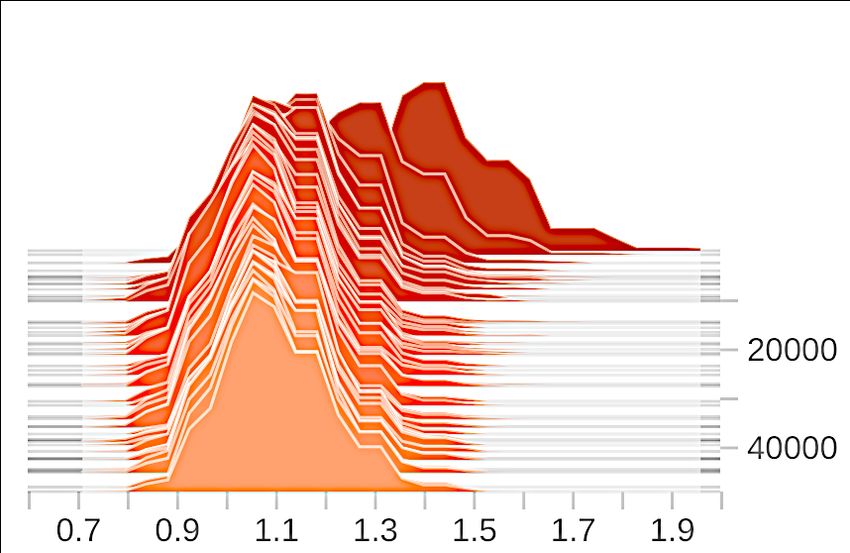
Effects of gradient clipping. We show in Figure A1 the gradient norm distribution before and after
gradient clipping. The clipping bound is set to be 1.1 for DP-SGD and 1 for our method. In contrast
to DP-SGD, the clipping operation distorts less information in our framework, witnessed by a much
smaller difference in the average gradient norm before and after the clipping. Moreover, the gradients
used in our method exhibit much less variance both before and after the clipping compared with
DP-SGD.
(a) DP-SGD (before) (b) DP-SGD (after) (c) Ours (before) (d) Ours (after)
Figure A1: Effects of gradient clipping.
Comparison to Baselines. We provide the detailed quantitative results in Table A1 and A2, which
are supplementary to Table 1 in the main paper. We show in parentheses the calibrated accuracy,
i.e., the absolute accuracy of each classifier trained on generated data divided by the accuracy when
trained on real data. The results are averaged over five runs.
Privacy-utility Curves. We show in Figure A2 the privacy-utility curves of different methods when
applied to the Fashion-MNIST dataset. We evaluate over three runs and show the corresponding
mean and standard deviation. Similar to the results shown in Figure 4 in the main paper, our method
achieves a consistent improvement over prior methods across a broad range of privacy budget ε.
4
https://github.com/frhrdr/Differentially-Private-Mean-Embeddings-with-Random-
Features-for-Synthetic-Data-Generation
5
https://github.com/reihaneh-torkzadehmahani/DP-CGAN
6
https://bitbucket.org/mvdschaar/mlforhealthlabpub/src/2534877d99c8fdf19cbade16057990171e249ef3/
alg/pategan/
16Real GAN (non-private) G-PATE DP-SGD GAN DP-Merf DP-Merf AE Ours
MLP 0.98 0.84 (85%) 0.25 (26%) 0.60 (61%) 0.63 (64%) 0.54 (55%) 0.79 (81%)
CNN 0.99 0.84 (85%) 0.51 (52%) 0.64 (65%) 0.63 (64%) 0.68 (69%) 0.80 (81%)
adaboost 0.73 0.28 (39%) 0.11 (16%) 0.32 (44%) 0.38 (52%) 0.21 (29%) 0.21 (29%)
bagging 0.93 0.46 (49%) 0.36 (38%) 0.44 (47%) 0.43 (46%) 0.33 (35%) 0.45 (48%)
bernoulli nb 0.84 0.80 (95%) 0.71 (84%) 0.62 (74%) 0.76 (90%) 0.50 (60%) 0.77 (92%)
decision tree 0.88 0.40 (45%) 0.13 (14%) 0.36 (41%) 0.29 (33%) 0.27 (31%) 0.35 (40%)
gaussian nb 0.56 0.71 (126%) 0.61 (110%) 0.37 (66%) 0.57 (102%) 0.17 (30%) 0.64 (114%)
gbm 0.91 0.50 (55%) 0.11 (12%) 0.45 (49%) 0.36 (40%) 0.20 (22%) 0.39 (43%)
lda 0.88 0.84 (95%) 0.60 (68%) 0.59 (67%) 0.72 (82%) 0.55 (63%) 0.78 (89%)
linear svc 0.92 0.81 (88%) 0.24 (26%) 0.56 (61%) 0.58 (63%) 0.43 (47%) 0.76 (83%)
logistic reg 0.93 0.83 (90%) 0.26 (28%) 0.60 (65%) 0.66 (71%) 0.55 (59%) 0.79 (85%)
random forest 0.97 0.39 (41%) 0.33 (34%) 0.63 (65%) 0.66 (68%) 0.45 (46%) 0.52 (54%)
xgboost 0.91 0.44 (49%) 0.15 (16%) 0.60 (66%) 0.70 (77%) 0.54 (59%) 0.50 (55%)
Average 0.88 0.63 (71%) 0.34 (40%) 0.52 (59%) 0.57 (66%) 0.42 (47%) 0.60 (69%)
Table A1: Classification accuracy on MNIST (ε = 10, δ = 10−5 ).
Real GAN (non-private) G-PATE DP-SGD GAN DP-Merf DP-Merf AE Ours
MLP 0.88 0.77 (88%) 0.30 (34%) 0.50 (57%) 0.56 (64%) 0.56 (64%) 0.65 (74%)
CNN 0.91 0.73 (80%) 0.50 (54%) 0.46 (51%) 0.54 (59%) 0.62 (68%) 0.64 (70%)
adaboost 0.56 0.41 (74%) 0.42 (75%) 0.21 (38%) 0.33 (59%) 0.26 (46%) 0.25 (45%)
bagging 0.84 0.57 (68%) 0.38 (45%) 0.32 (38%) 0.40 (47%) 0.45 (54%) 0.47 (56%)
bernoulli nb 0.65 0.59 (91%) 0.57 (88%) 0.50 (77%) 0.62 (95%) 0.54 (83%) 0.55 (85%)
decision tree 0.79 0.53 (67%) 0.24 (30%) 0.33 (42%) 0.25 (32%) 0.36 (46%) 0.40 (51%)
gaussian nb 0.59 0.55 (93%) 0.57 (97%) 0.28 (47%) 0.59 (100%) 0.12 (20%) 0.48 (81%)
gbm 0.83 0.44 (53%) 0.25 (30%) 0.38 (46%) 0.27 (33%) 0.30 (36%) 0.38 (46%)
lda 0.80 0.77 (96%) 0.55 (69%) 0.55 (69%) 0.67 (84%) 0.65 (81%) 0.67 (84%)
linear svc 0.84 0.77 (91%) 0.30 (36%) 0.39 (46%) 0.46 (55%) 0.40 (48%) 0.65 (77%)
logistic reg 0.84 0.76 (90%) 0.35 (42%) 0.51 (61%) 0.59 (70%) 0.50 (60%) 0.68 (81%)
random forest 0.88 0.69 (78%) 0.33 (37%) 0.51 (58%) 0.61 (69%) 0.55 (63%) 0.54 (61%)
xgboost 0.83 0.65 (78%) 0.49 (59%) 0.52 (63%) 0.62 (75%) 0.55 (66%) 0.47 (57%)
Average 0.79 0.61 (77%) 0.40 (54%) 0.42 (53%) 0.50 (65%) 0.45 (56%) 0.53 (67%)
−5
Table A2: Classification accuracy on Fashion-MNIST (ε = 10, δ = 10 ).
Noise scale Iterations
8 8
7 7
6 6
5 5
IS (↑) 4 IS (↑) 4
3 3
2 2
1 1
0 0
2 4 6 8 10 12 14 16 18 20 0 2 5 7 10 12 15 17 20
epsilon epsilon
300 450
275 400
250
350
225
300
FID (↓) 200 FID (↓)
250
175
200
150
150
125
100
100
2 4 6 8 10 12 14 16 18 20 0 2 5 7 10 12 15 17 20
epsilon epsilon
DP-Merf DP-Merf AE DP-SGD GAN Ours
Figure A2: Privacy-utility trade-off on Fashion-MNIST with δ = 10−5 . (Left: Effects of noise scale.
Right: Effects of Iterations.)
17You can also read