CHAMELEON: LEARNING MODEL INITIALIZATIONS ACROSS TASKS WITH DIFFERENT SCHEMAS
←
→
Page content transcription
If your browser does not render page correctly, please read the page content below
Under review as a conference paper at ICLR 2021

C HAMELEON : L EARNING M ODEL I NITIALIZATIONS
ACROSS TASKS W ITH D IFFERENT S CHEMAS
 Anonymous authors
 Paper under double-blind review

                                              A BSTRACT

         Parametric models, and particularly neural networks, require weight initialization
         as a starting point for gradient-based optimization. Recent work shows that an
         initial parameter set can be learned from a population of supervised learning tasks
         that enables a fast convergence for unseen tasks even when only a handful of
         instances is available (model-agnostic meta-learning). Currently, methods for
         learning model initializations are limited to a population of tasks sharing the
         same schema, i.e., the same number, order, type, and semantics of predictor and
         target variables. In this paper, we address the problem of meta-learning weight
         initialization across tasks with different schemas, for example, if the number of
         predictors varies across tasks, while they still share some variables. We propose
         Chameleon, a model that learns to align different predictor schemas to a common
         representation. In experiments on 23 datasets of the OpenML-CC18 benchmark,
         we show that Chameleon can successfully learn parameter initializations across
         tasks with different schemas, presenting, to the best of our knowledge, the first
         cross-dataset few-shot classification approach for unstructured data.

1    I NTRODUCTION

Humans require only a few examples to correctly classify new instances of previously unknown
objects. For example, it is sufficient to see a handful of images of a specific type of dog before
being able to classify dogs of this type consistently. In contrast, deep learning models optimized
in a classical supervised setup usually require a vast number of training examples to match human
performance. A striking difference is that a human has already learned to classify countless other
objects, while parameters of a neural network are typically initialized randomly. Previous approaches
improved this starting point for gradient-based optimization by choosing a more robust random
initialization (He et al., 2015) or by starting from a pretrained network (Pan & Yang, 2010). Still,
models do not learn from only a handful of training examples even when applying these techniques.
Moreover, established hyperparameter optimization methods (Schilling et al., 2016) are not capable
of optimizing the model initialization due to the high-dimensional parameter space. Few-shot
classification aims at correctly classifying unseen instances of a novel task with only a few labeled
training instances given. This is typically accomplished by meta-learning across a set of training
tasks, which consist of training and validation examples with given labels for a set of classes. The
field has gained immense popularity among researchers after recent meta-learning approaches have
shown that it is possible to learn a weight initialization across different tasks, which facilitates a faster
convergence speed and thus enables classifying novel classes after seeing only a few instances (Finn
et al., 2018). However, training a single model across different tasks is only feasible if all tasks share
the same schema, meaning that all instances share one set of features in identical order. For that
reason, most approaches demonstrate their performance on image data, which can be easily scaled to
a fixed shape, whereas transforming unstructured data to a uniform schema is not trivial.
We want to extend popular approaches to operate invariant of schema, i.e., independent of order and
shape, making it possible to use meta-learning approaches on unstructured data with varying feature
spaces, e.g., learning a model from heart disease data that can accurately classify a few-shot task for
diabetes detection that relies on similar features. Thus, we require a schema-invariant encoder that
maps heart disease and diabetes data to one feature representation, which then can be used to train a
single model via popular meta-learning algorithms like REPTILE (Nichol et al., 2018b).

                                                     1
Under review as a conference paper at ICLR 2021
Original Task Schema Transformed Task Schema
Task A
ŷA
Task B Chameleon
Common Schema Model M ŷB
Task C
ŷC
Figure 1: Chameleon Pipeline: Chameleon aims to encode tasks with different schemas to a shared representa-
tion with an uniform feature space, which can then be processed by any classifier. The left block represents tasks
of the same domain with different schemas. The middle represents the aligned features in a fixed schema.
We propose a set-wise feature transformation model called CHAMELEON, named after a REPTILE
capable of adjusting its colors according to the environment in which it is located. CHAMELEON
projects different schemas to a fixed input space while keeping features from different tasks but of
the same type or distribution in the same position, as illustrated by Figure 1. Our model learns to
compute a task-specific reordering matrix that, when multiplied with the original input, aligns the
schema of unstructured tasks to a common representation while behaving invariant to the order of
input features.
Our main contributions are as follows: (1) We show how our proposed method CHAMELEON can
learn to align varying feature spaces to a common representation. (2) We propose the first approach
to tackle few-shot classification for tasks with different schemas. (3) In experiments on 23 datasets
of the OpenML-CC18 benchmark (Bischl et al., 2017) collection, we demonstrate how current
meta-learning approaches can successfully learn a model initialization across tasks with different
schemas as long as they share some variables with respect to their type or semantics. (4) Although an
alignment makes little sense to be performed on top of structured data such as images which can be
easily rescaled, we demonstrate how CHAMELEON can align latent embeddings of two image datasets
generated with different neural networks.
2 R ELATED W ORK
Our goal is to extend recent few-shot classification approaches that make use of optimization-based
meta-learning by adding a feature alignment component that casts different inputs to a common
schema, presenting the first approach working across tasks with different schema. In this section, we
will discuss various works related to our approach.
Research on transfer learning (Pan & Yang, 2010; Sung et al., 2018; Gligic et al., 2020) has shown
that training a model on different auxiliary tasks before actually fitting it to the target problem can
provide better results if training data is scarce. Motivated by this, few-shot learning approaches try to
generalize to novel tasks with unseen classes given only a few instances by first meta-learning across
a set of training tasks (Duan et al., 2017; Finn et al., 2017b; Snell et al., 2017). A task τ consists of
predictor data Xτ , a target Yτ , a predefined training/test split τ = (Xτtrain , Yτtrain , Xτtest , Yτtest ) and a
loss function Lτ . Typically, an N -way K-shot problem refers to a few-shot learning problem where
each task consists of N classes with K training samples per class.
Heterogeneous Transfer Learning tries to tackle a similar problem setting as described in this work.
In contrast to regular Transfer Learning, the feature spaces of the auxiliary tasks and the actual
task differ and are often non-overlapping (Day & Khoshgoftaar, 2017). Many approaches require
co-occurence data i.e. instances that can be found in both datasets (Wu et al., 2019; Qi et al., 2011),
rely on jointly optimizing separate models for each dataset to propagate information (Zhao & Hoi,
2010; Yan et al., 2016), or utilize meta-features (Feuz & Cook, 2015). Oftentimes, these approaches
operate on structured data e.g. images and text with different data distributions for the tasks at hand
(Li et al., 2019; He et al., 2019). These datasets can thus be embedded in a shared space with standard
models such as convolutional neural networks and transformer-based language models. However,
none of these approaches are capable of training a single encoder that operates across a meta-dataset
of tasks with different schema for unstructured data.
2Under review as a conference paper at ICLR 2021
Early approaches like (Fe-Fei et al., 2003) already investigated the few-shot learning setting by
representing prior knowledge as a probability density function. In recent years, various works
proposed new model-based meta-learning approaches which rapidly improved the state-of-the-art
few-shot learning benchmarks. Most prominently, this includes methods which rely on learning
an embedding space for non-parametric metric approaches during inference time (Vinyals et al.,
2016; Snell et al., 2017), and approaches which utilize an external memory which stores information
about previously seen classes (Santoro et al., 2016; Munkhdalai & Yu, 2017). Several more recent
meta-learning approaches have been developed which introduce architectures and parameterization
techniques specifically suited for few-shot classification (Mishra et al., 2018; Shi et al., 2019; Wang &
Chen, 2020) while others try to extract useful meta-features from datasets to improve hyper-parameter
optimization (Jomaa et al., 2019).
In contrast, Finn et al. (2017a) showed that an optimization-based approach, which solely adapts the
learning paradigm can be sufficient for learning across tasks. Model Agnostic Meta-Learning (MAML)
describes a model initialization algorithm that is capable of training an arbitrary model f across
different tasks. Instead of sequentially training the model one task at a time, it uses update steps from
different tasks to find a common gradient direction that achieves a fast convergence. In other words,
for each meta-learning update, we would need an initial value for the model parameters θ. Then, we
sample a batch of tasks T , and for each task τ ∈ T we find an updated version of θ using N examples
from the task by performing gradient descent with learning rate α as in: θτ0 ← θ − α∇θ Lτ (fθ ). The
final update of θ with step size β will be:
1 X
θ ←θ−β ∇θ Lτ (fθτ0 ) (1)
|T | τ
Finn et al. (2017a) state that MAML does not require learning an update rule (Ravi & Larochelle,
2016), or restricting their model architecture (Santoro et al., 2016). They extended their approach
by incorporating a probabilistic component such that for a new task, the model is sampled from a
distribution of models to guarantee a higher model diversification for ambiguous tasks (Finn et al.,
2018). However, MAML requires to compute second-order derivatives, resulting in a computationally
heavy approach. Nichol et al. (2018b) extend upon the first-order approximation given as an ablation
by Finn et al. (2018), which numerically approximates Equation (1) by replacing the second derivative
with the weights difference, s.t. the update rule used in REPTILE is given by:
1 X 0
θ ←θ−β (θ − θ) (2)
|T | τ τ
which means we can use the difference between the previous and updated version as an approximation
of the second-order derivatives to reduce computational cost. The serial version is presented in
Algorithm (1).1 All of these approaches rely on a fixed schema, i.e. the same set of features with
identical alignment across all tasks. However, many similar datasets only share a subset of their
features, while oftentimes having a different order or representation e.g. latent embeddings for
two different image datasets generated by training two similar architectures. Most current few-shot
classification approaches sample tasks from a single dataset by selecting a random subset of classes;
although it is possible to train a single meta-model on two different image datasets as shown by
Munkhdalai & Yu (2017) and Tseng et al. (2020) since the images can be scaled to a fixed size.
Further research demonstrates that it is possible to learn a single model across different output sizes
(Drumond et al., 2020). Recently, a meta-dataset for few-shot classification of image tasks was also
published to promote meta-learning across multiple datasets (Triantafillou et al., 2020). Optimizing
a single model across various datasets requires a shared feature space. Thus, it is required to align
the features which is achieved by simply rescaling all instances in the case of image data which is
not trivial for unstructured data. Recent work relies on preprocessing images to a one-dimensional
latent embedding with an additional deep neural network. The authors Rusu et al. (2019) train a
Wide Residual Network (Zagoruyko & Komodakis, 2016) on the meta-training data of MiniImageNet
(Vinyals et al., 2016) to compute latent embeddings of the data which are then used for few-shot
classification, demonstrating state-of-the-art results.
Finding a suitable initialization for deep network has long been a focus of machine learning research.
Especially the initialization of Glorot & Bengio (2010) and later He et al. (2015) which emphasize
1
Note that REPTILE does not require validation instances during meta-learning.
3Under review as a conference paper at ICLR 2021
the importance of a scaled variance that depends on the layer inputs are widely used. Similar findings
are also reported by Cao et al. (2019). Recently, Dauphin & Schoenholz (2019) showed that it is
possible to learn a suitable initialization by optimizing the norms of the respective weights. So far,
none of these methods tried to learn a common initialization across tasks with different schema.
We propose a novel feature alignment component named CHAMELEON, which enables state-of-the-art
methods to learn how to work on top of tasks whose feature vector differ not only in their length
but also their concrete alignment. Our model shares resemblance with scaled dot-product attention
popularized by (Vaswani et al., 2017):
QK T
Attention(Q, K, V ) = sof tmax( √ )V (3)
dK
where Q, K and V are matrices describing queries, keys and values, and dK is the dimensionality of
the keys such that the softmax computes an attention mask which is then multiplied with the values V .
In contrast to this, we pretrain the parametrized model CHAMELEON to compute a soft permutation
matrix which can realign features across tasks with varying schema when multiplied with V instead
of computing a simple attention mask.
Algorithm 1 REPTILE Nichol et al. (2018b)
Input: Meta-dataset T = {(X1 , Y1 , L1 ), ..., (X|T | , Y|T | , L|T | )}, learning rate β
1: Randomly initialize parameters θ of model f
2: for iteration = 1, 2, ... do
3: Sample task (Xτ , Yτ , Lτ ) ∼ T
4: θ0 ← θ
5: for k steps = 1,2,... do
6: θ0 ← θ0 − α∇θ0 Lτ (Yτ , f (Xτ ; θ0 ))
7: end for
8: θ ← θ − β(θ0 − θ)
9: end for
10: return parameters θ of model f
3 M ETHODOLOGY
3.1 P ROBLEM SETTING
We describe a classification dataset with vector-shaped predictors (i.e., no images, time series
etc.) by a pair (X, Y ) ∈ RN ×F × {0, ..., C}N , with predictors X and targets Y , where N
denotes theSnumber of instances, F the number of predictors and C the number of classes.
Let DFS:= N ∈N RN ×F × {0, ..., C}N be the space of all such datasets with F predictors and
D := F ∈N DF be the space of any such dataset. Let us also denote the space of all predictor
matrices with F predictors by XF := N ∈N RN ×F and all predictor matrices by X := F ∈N XF .
S S
Then a dataset τ = (X, Y ) ∈ D equipped with a predefined training/test split, i.e. the quadruplet
τ = (Xτtrain , Yτtrain , Xτtest , Yτtest ) is called a task. A collection of such tasks T ⊂ D is called a meta-
dataset. Similar to splitting a single data set into a training and test part, one can split a meta-dataset
T = T train ∪˙ T test . The schema of a task τ then describes not only the number and order, but also the
semantics of predictor variables {pτ1 , pτ2 , . . . , pτF } in Xτtrain .
Consider a meta-dataset of correlated tasks T ⊂ D, such that the predictor variables
{pτ1 , pτ2 , . . . , pτF } of any individual task τ are contained in a common set of predictor variables
{p1 , p2 , . . . , pK }. Methods like REPTILE and MAML try to find the best initialization for a specific
model, in this work referred to as ŷ, to operate on a set T of similar tasks. However, every task τ
has to share the same schema of common size K, where similar features shared across tasks are in
the same position. A feature-order invariant encoder is needed to map the data representation Xτ of
tasks with varying input schema and feature length Fτ to a shared latent representation X fτ with fixed
feature length K:
enc : X −→ XK , Xτ ∈ RN ×Fτ 7−→ X eτ ∈ RN ×K (4)
4Under review as a conference paper at ICLR 2021
Chameleon
Input Xτ: Output
Fτ × 16
Fτ × K
Π(Xτ)
Fτ × N
XτΠ(Xτ):
Fτ × 8
(N×16×1)
Transpose
+ Softmax
Conv1D
(N×8×1)
Conv1D
(N×K×1)
Conv1D
N × Fτ
N×K
Figure 2: The Chameleon Architecture: N represents the number of samples in τ , Fτ is the number of features
in τ , and K is the number of features in the desired feature space. “Conv(a × b × c)” is a convolution operation
with a input channels, filter size of b and kernel length c.
where N represents the number of instances in Xτ , Fτ is the number of features of task τ which
varies across tasks, and K is the size of the desired feature space. By combining this encoder
with model ŷ that works on a fixed input size K and outputs the predicted target e.g. binary
classification, it is possible to apply the REPTILE algorithm to learn an initialization θinit across tasks
with different schema. The optimization objective then becomes the meta-loss for the combined
network f = ŷ ◦ enc over a set of tasks T :
argmin Eτ ∼T Lτ Yτtest , f Xτtest ; θτ(u) s.t. θτ(u) = A(u) Xτtrain , Yτtrain , Lτ , f ; θinit (5)
θ init
where θinit is the set of initial weights for the combined network f consisting of enc with parameters
(u)
θenc and model ŷ with parameters θŷ , and θτ are the updated weights after applying the learning
procedure A for u iterations on the task τ as defined in Algorithm 1 for the inner updates of REPTILE.
It is important to mention that learning one weight parameterization across any heterogeneous set of
tasks is extremely difficult since it is most likely impossible to find one initialization for two tasks
with a vastly different number and type of features. By contrast, if two tasks share similar features,
one can align the similar features to a common representation so that a model can directly learn
across different tasks by transforming the tasks as illustrated in Figure 1.
3.2 C HAMELEON
Consider a set of tasks where a right stochastic matrix Πτ exists for each task that reorders predictor
data Xτ into Xeτ having the same schema for every task τ ∈ T :
eτ = Xτ · Πτ , where
X (6)
x̃1,1 ... x̃1,K x1,1 . . . x1,Fτ π1,1 ... π1,K
.. .. .. = .. . .. .. · ...
. .. ..
. . . . . .
x̃N,1 ... x̃N,K xN,1 . . . xN,Fτ πFτ ,1 ... πFτ ,K
| {z } | {z } | {z }
X
eτ Xτ Πτ
Every xm,n represents the feature n of sample m. Every πm,n represent how much of feature m
(from samples in Xτ ) should be shifted to position n in the adapted input X eτ . Finally, every x̃m,n
represent the new feature n of sample m in Xτ with the adpated shape and size. In order to achieve
the same X eτ when permuting two features of a task Xτ , we must simply permute the corresponding
rows in Πτ to achieve the same X eτ . Since Πτ is a right stochastic matrix, the summation for every
P
row of Πτ is set to be equal to 1 as in i πj,i = 1, so that each value in Πτ simply states how much a
feature is shifted to a corresponding position. For example: Consider that task a has features [apples,
bananas, melons] and task b features [lemons, bananas, apples]. Both can be transformed to the
same representation [apples, lemons, bananas, melons] by replacing missing features with zeros and
reordering them. This transformation must have the same result for a and b independent of their
feature order. In a real life scenario, features might come with different names or sometimes their
similarity is not clear to the human eye. Note that a classic autoencoder is not capable of this as it is
not invariant to the order of the features. Our proposed component, denoted by Φ, takes a task as
5Under review as a conference paper at ICLR 2021
input and outputs the corresponding reordering matrix:
Φ(Xτ , θenc ) = Π̂τ (7)
The function Φ is a neural network parameterized by θenc . It consists of three 1D-convolutions,
where the last one is the output layer that estimates the alignment matrix via a softmax activation.
The input is first transposed to size [Fτ × N ] (where N is the number of samples) i.e., each feature is
represented by a vector of instances. Each convolution has kernel length 1 (as the order of instances
is arbitrary and thus needs to be permutation invariant) and a channel output size of 8, 16, and lastly
K. The result is a reordering matrix displaying the relation of every original feature to each of the K
features in the target space. Each of these vectors passes through a softmax layer, computing the ratio
of features in Xτ shifted to each position of X eτ . Finally, the reordering matrix can be multiplied
with the input to compute the aligned task as defined in Equation (6). By using a kernel length
of 1 in combination with the final matrix multiplication, the full architecture becomes permutation
invariant in the feature dimension. Column-wise permuting the features of an input task leads to
the corresponding row-wise permutation of the reordering matrix. Thus, multiplying both matrices
results in the same aligned output independent of permutation. The overall architecture can be seen
in Figure 2. The encoder necessary for training across tasks with different predictor vectors with
REPTILE by optimizing Equation (5) is then given as:
enc : Xτ 7−→ Xτ · Φ(Xτ , θenc ) = Xτ · Π̂τ (8)
3.3 R EORDERING T RAINING
Only joint-training the network ŷ ◦ enc as described above, will not teach CHAMELEON denoted
by Φ how to reorder the features to a shared representation. That is why it is necessary to train Φ
specifically with the objective of reordering features (reordering training). In order to do so, we
optimize Φ to align novel tasks by training on a set of tasks for which the reordering matrix Πτ
exists such that it maps τ to the shared representation. In other words, we require a meta-dataset
that contains not only a set of similar tasks τ ∈ T with different schema, but also the position for
each feature in the shared representation given by a permutation matrix. If Πτ is known beforehand
for each τ ∈ T , optimizing Chameleon becomes a simple supervised classification task based on
predicting the new position of each feature in τ . Thus, we can minimize the expected reordering loss
over the meta-dataset:
θenc = argmin Eτ ∼T LΦ Πτ , Π̂τ (9)
θenc
where LΦ is the softmax cross-entropy loss, Πτ is the ground-truth (one-hot encoding of the new
position for each variable), and Π̂τ is the prediction. This training procedure can be seen in Algo-
rithm (2). The trained CHAMELEON model can then be used to compute the Πτ for any unseen task
τ ∈T.
Algorithm 2 Reordering Training
Input: Meta-dataset T = {(X1 , Π1 ), ..., (X|T | , Π|T | )}, latent dimension K, learning rate γ
1: Randomly initialize parameters θenc of the CHAMELEON model
2: for training iteration = 1, 2, ... do
3: randomly sample τ ∼ T
4: θenc ←− θenc − γ∇LΦ (Πτ , Φ(Xτ , θenc ))
5: end for
6: return Trained parameters θenc of the CHAMELEON model
After this training procedure, we can use the learned weights as initialization for Φ before optimizing
ŷ ◦ enc with REPTILE without further using LΦ . Experiments show that this procedure improves our
results significantly compared to only optimizing the joint meta-loss.
Training the CHAMELEON component to reorder similar tasks to a shared representation not only
requires a meta-dataset but one where the true reordering matrix Πτ is provided for every task. In
application, this means manually matching similar features of different training tasks so that novel
tasks can be matched automatically. However, it is possible to sample a broad number of tasks from a
6Under review as a conference paper at ICLR 2021
(a) Split (b) No-Split
Accuracy increase in neg. log scale
0.2 0.2
0.4 0.4
0.6 0.6
0.8 0.8 y (Reptile Padded)
(Reptile Padded) y enc (Proposed)
1.0 enc (Proposed) 1.0 Oracle
tic
phoneme
analcat
jungle
cmc
electricity
wine
wilt
vowel
ilpd
wall
Magic
pendigits
abalone
letter
diabetes
Gesture
vehicle
segment
mfeat
wdbc
tic
analcat
cmc
electricity
jungle
wine
wall
vowel
blood
letter
phoneme
pendigits
Gesture
vehic
Magic
banknote
wilt
ilpd
diabetes
abalone
mfeat
segment
wdbc
Figure 3: Accuracy improvement for each method over Glorot initialization (Glorot & Bengio, 2010): The
difference is plotted in negative log scale to account for the varying performance scales across the different
datasets (higher points are better; A value of −1 is equivalent to the Glorot initialization). The graph (a)
represents Split experiments while (b) depicts the No-Split experiments. Notice that the oracle has been omitted
from the Split experiments since there is no true feature alignment for unseen features. The dataset axis is sorted
by the performance of REPTILE on the base model to improve readability. All results are averaged over 5 runs.
single dataset by sampling smaller sub-tasks from it, selecting a random subset of features in arbitrary
order for N random instances. Thus, it is not necessary to manually match the features since all these
sub-tasks share the same Π̂τ apart from the respective permutation of the rows as mentioned above.
4 E XPERIMENTAL R ESULTS
Baseline and Setup In order to evaluate the proposed method, we investigate the combined model
ŷ ◦ enc with the initialization for enc obtained by pretraining CHAMELEON as defined in Equation 9
before using REPTILE to jointly optimize ŷ ◦ enc. We compare the performance with an initialization
obtained by running REPTILE on the base model ŷ by training on tasks padded to a fixed size K
as ŷ is not schema invariant. Both initializations are then compared to the performance of model ŷ
with random Glorot initialization (Glorot & Bengio, 2010) (referred to as Random). In all of our
experiments, we measure the performance of a model and its initialization by evaluating the validation
data of a task after performing three update steps on the respective training data. All experiments
are conducted in two variants: In Split experiments, test tasks contain novel features in addition to
features seen during meta-training. In contrast, test tasks in No-Split experiments only consist of
features seen during meta-training. While the Split experiments evaluate the performance of the
model when faced with novel features during meta-testing, the No-Split experiments can be used to
compare against a perfect alignment by repeating the baseline experiment with tasks that are already
aligned (referred to as Oracle). A detailed description of the utilized models is found in Appendix B.
Meta-Datasets For our main experiments, we utilize a single dataset as meta-dataset by sampling
the training and test tasks from it. This allows us to evaluate our method on different domains without
matching related datasets since Π̂τ is naturally given for a subset of permuted features. Novel features
can also be introduced during testing by splitting not only the instances but also the features of a
dataset in train and test partition (Split). Training tasks are then sampled by selecting a random subset
of the training features in arbitrary order for N instances. Stratified sampling guarantees that test tasks
contain both features from train and test while sampling the instances from the test set only. For all
experiments, 75% of the instances are used for reordering training of CHAMELEON and joint-training
of the full architecture, and 25% for sampling test tasks. For Split experiments, we further impose a
train-test split on the features (20% of the features are restricted to the test split). Our work is built
on top of REPTILE (Nichol et al., 2018b) but can be used in conjunction with any model-agnostic
meta-learning method. We opted to use REPTILE since it does not require second-order derivatives,
and the code is publicly available (Nichol et al., 2018a) while also being easy to adapt to our problem.
7Under review as a conference paper at ICLR 2021
5 4 3 2 1 6 5 4 3 2 1
ŷ Random ŷ ◦ enc Proposed ŷ Random ŷ Oracle
ŷ Reptile Padded ŷ ◦ enc Frozen ŷ Reptile Padded ŷ ◦ enc Proposed
ŷ ◦ enc Untrain ŷ ◦ enc Untrain ŷ ◦ enc Frozen
Figure 4: Critical Difference Diagram for Split (Left) and No-Split (Right) showing results of Wilcoxon
signed-rank test with Holm’s alpha correction and 5% significance level. Models are ranked by their performance
and a thicker horizontal line indicates pairs that are not statistically different.
Main Results We evaluate our approach using the OpenML-CC18 benchmark (Bischl et al., 2017)
from which we selected 23 datasets for few-shot classification. The details of all datasets utilized in
this work are summarized in Appendix B. The results in Figure 3 display the model performance
after performing three update steps on a novel test task to illustrate the faster convergence. The graph
shows a clear performance lift when using the proposed architecture after pretraining it to reorder
tasks. This demonstrates to the best of our knowledge the first few-shot classification approach,
which successfully learns across tasks with varying schemas (contribution 2). Furthermore, in the
No-Split results one can see that the performance of the proposed method approaches the Oracle
performance, which suggests an ideal feature alignment. When adding novel features during test time
(Split) CHAMELEON is still able to outperform the other setups although with a lower margin.
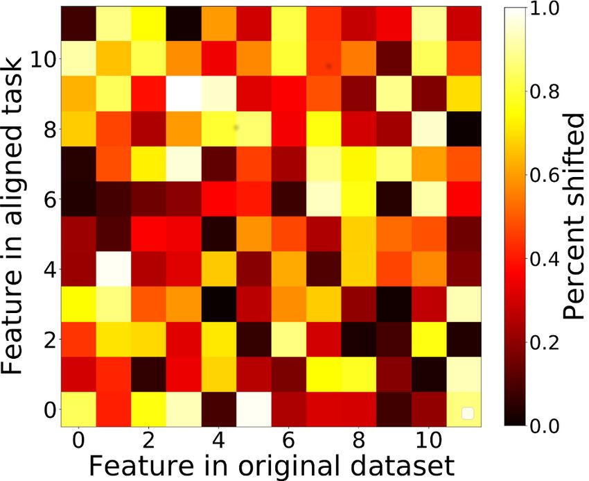
Ablations We visualize the result of pretraining CHAMELEON on the Wine dataset (from OpenML-
CC18) in Figure 6 to show that the proposed model is capable of learning the correct alignment
between tasks. One can see that the component manages to learn the true feature position in almost
all cases. Moreover, this illustration does also show that CHAMELEON can be used to compute the
similarity between different features by indicating which pairs are confused most often. For example,
features two and four are showing a strong correlation, which is very plausible since they depict the
free sulfur dioxide and total sulfur dioxide level of the wine. This demonstrates that our proposed
architecture is able to learn an alignment between different feature spaces (contribution 1).
Furthermore, we repeat the experiments on the OpenML-CC18 benchmark in two ablation studies to
measure the impact of joint-training and the proposed reordering training (Algorithm 2). First, we
do not train CHAMELEON with Equation 9, but only jointly train ŷ ◦ enc with REPTILE to evaluate
the influence of adding additional parameters to the network without pretraining it. Secondly, we
use REPTILE only to update the initialization for the parameters of ŷ while freezing the pretrained
parameters of enc in order to assess the effect of joint-training both network components. These
two variants are referred to as Untrain and Frozen. We compare these ablations to our approach by
conducting a Wilcoxon signed-rank test (Wilcoxon, 1992) with Holm’s alpha correction (Holm, 1979).
The results are displayed in the form of a critical difference diagram (Demšar, 2006; Ismail Fawaz
et al., 2019) presented in Figure 4. The diagram shows the ranked performance of each model and
whether they are statistically different. The results confirm that our approach leads to statistically
significant improvements over the random and REPTILE baselines when pretraining CHAMELEON.
Similarly, our approach is also significantly better than jointly training the full architecture without
pretraining CHAMELEON (UNTRAIN), confirming that the improvements do not stem from the
increased model capacity. Finally, comparing the results to the FROZEN model shows improvements
that are not significant, indicating that a near-optimal alignment was already found during pretraining.
A detailed overview for all experimental results is given in Appendix C.
Latent Embeddings Experiments Learning to align features is only feasible for unstructured data
since this approach would not preserve any structure. However, it is a widespread practice among
few-shot classification methods, and computer vision approaches in general, to use a pretrained
model to embed image data into a latent space before applying further operations. We can use
CHAMELEON to align the latent embeddings of image datasets that are generated with different
networks. Thus, it is possible to use latent embeddings for meta-training while evaluating on novel
tasks that are not yet embedded in case the embedding network is not available, or the complexity of
different datasets requires models with different capacities to extract useful features. We conduct
an additional experiment for which we combine two similar image datasets, namely EMNIST-Digits
and EMNIST-Letters (Cohen et al., 2017). Similar to the work of Rusu et al. (2019), we train one
neural network on each dataset in order to generate similar latent embeddings with different schema,
namely 32 and 64 latent features. Afterward, we can sample training tasks from one embedding while
8Under review as a conference paper at ICLR 2021
results
0.36
Accuracy after 3 update steps
0.34
0.32
0.30
0.28
0.26
random
0.24
enc
0.22 enc (Ablation: Untrain)
enc (Ablation: Frozen)
0 4000 8000 12000 16000 20000
Meta-epochs Figure 6: Heat map of the feature shifts for
the Wine data computed with CHAMELEON af-
Figure 5: Latent embedding results. Meta test ac- ter reordering-training: The x-axis represents the
curacy on the EMNIST-Digits data set while training twelve features of the original dataset in the correct
on EMNIST-Letters. Each point represents the ac- order and the y-axis shows which position these fea-
curacy on the 1600 test tasks after performing three tures are shifted to when presented in a permuted
update steps on the respective training data. Results subset.
are averaged over 5 runs.
evaluating on tasks sampled from the other one. In the combined experiments, the full training is
performed on the EMNIST-Letters dataset, while EMNIST-Digits is used for testing. Splitting the
features is not necessary as the train, and test features are coming from different datasets. The results
of this experiment are displayed in Figure 5. It shows the accuracy of EMNIST-Digits averaged across
5 runs with 1,600 generated tasks per run during the REPTILE training on EMNIST-Letters for the
different model variants. Each test task is evaluated by performing 3 update steps on the training
samples and measuring the accuracy of its validation data afterward. One can see that our proposed
approach reports a significantly higher accuracy than the REPTILE baseline after performing three
update steps on a task (contribution 4). Thus, showing that CHAMELEON is able to transfer knowledge
from one dataset to another. Moreover, simply adding CHAMELEON without pretraining it to reorder
tasks (Untrain) does not lead to any improvement. This might be sparked by using a CHAMELEON
component that has a much lower number of parameters than the base network. Only by adding the
reordering-training, the model manages to converge to a suitable initialization. In contrast to our
experiments on the OpenML datasets, freezing the weights of CHAMELEON after pretraining also
fails to give an improvement, suggesting that the pretraining did not manage to capture the ideal
alignment, but enables learning it during joint-training. Our code is available at BLIND - REVIEW.
5 C ONCLUSION
In this paper, we presented, to the best of our knowledge, the first approach to tackle few-shot
classification for unstructured tasks with different schema. Our model component CHAMELEON is
capable of embedding tasks to a common representation by computing a matrix that can reorder
the features. For this, we propose a novel pretraining framework that is shown to learn useful
permutations across tasks in a supervised fashion without requiring actual labels. In experiments
on 23 datasets of the OpenML-CC18 benchmark, our method shows significant improvements even
when presented with features not seen during training. Furthermore, by aligning different latent
embeddings we demonstrate how a single meta-model can be used to learn across multiple image
datasets each embedded with a distinct network.
R EFERENCES
Bernd Bischl, Giuseppe Casalicchio, Matthias Feurer, Frank Hutter, Michel Lang, Rafael G Manto-
vani, Jan N van Rijn, and Joaquin Vanschoren. Openml benchmarking suites and the openml100,
2017.
9Under review as a conference paper at ICLR 2021
Weipeng Cao, Muhammed JA Patwary, Pengfei Yang, Xizhao Wang, and Zhong Ming. An initial
study on the relationship between meta features of dataset and the initialization of nnrw. In 2019
International Joint Conference on Neural Networks (IJCNN), pp. 1–8. IEEE, 2019.
Gregory Cohen, Saeed Afshar, Jonathan Tapson, and Andre Van Schaik. Emnist: Extending mnist to
handwritten letters, 2017.
Yann N Dauphin and Samuel Schoenholz. Metainit: Initializing learning by learning to initialize. In
Advances in Neural Information Processing Systems, pp. 12645–12657, 2019.
Oscar Day and Taghi M Khoshgoftaar. A survey on heterogeneous transfer learning. Journal of Big
Data, 4(1):29, 2017.
Janez Demšar. Statistical comparisons of classifiers over multiple data sets. Journal of Machine
learning research, 7(Jan):1–30, 2006.
Rafael Rego Drumond, Lukas Brinkmeyer, Josif Grabocka, and Lars Schmidt-Thieme. Hidra: Head
initialization across dynamic targets for robust architectures. In Proceedings of the 2020 SIAM
International Conference on Data Mining, pp. 397–405. SIAM, 2020.
Yan Duan, Marcin Andrychowicz, Bradly Stadie, OpenAI Jonathan Ho, Jonas Schneider, Ilya
Sutskever, Pieter Abbeel, and Wojciech Zaremba. One-shot imitation learning. In Advances in
neural information processing systems, pp. 1087–1098, 2017.
Li Fe-Fei et al. A bayesian approach to unsupervised one-shot learning of object categories. In
Proceedings Ninth IEEE International Conference on Computer Vision, pp. 1134–1141. IEEE,
2003.
Kyle D Feuz and Diane J Cook. Transfer learning across feature-rich heterogeneous feature spaces via
feature-space remapping (fsr). ACM Transactions on Intelligent Systems and Technology (TIST), 6
(1):1–27, 2015.
Chelsea Finn, Pieter Abbeel, and Sergey Levine. Model-agnostic meta-learning for fast adaptation of
deep networks. In Proceedings of the 34th International Conference on Machine Learning-Volume
70, pp. 1126–1135. JMLR. org, 2017a.
Chelsea Finn, Tianhe Yu, Tianhao Zhang, Pieter Abbeel, and Sergey Levine. One-shot visual imitation
learning via meta-learning. arXiv preprint arXiv:1709.04905, 2017b.
Chelsea Finn, Kelvin Xu, and Sergey Levine. Probabilistic model-agnostic meta-learning. In
Advances in Neural Information Processing Systems, pp. 9537–9548, 2018.
Luka Gligic, Andrey Kormilitzin, Paul Goldberg, and Alejo Nevado-Holgado. Named entity recog-
nition in electronic health records using transfer learning bootstrapped neural networks. Neural
Networks, 121:132–139, 2020.
Xavier Glorot and Yoshua Bengio. Understanding the difficulty of training deep feedforward neural
networks. In Proceedings of the thirteenth international conference on artificial intelligence and
statistics, pp. 249–256, 2010.
Kaiming He, Xiangyu Zhang, Shaoqing Ren, and Jian Sun. Delving deep into rectifiers: Surpassing
human-level performance on imagenet classification. In Proceedings of the IEEE international
conference on computer vision, pp. 1026–1034, 2015.
Xin He, Yushi Chen, and Pedram Ghamisi. Heterogeneous transfer learning for hyperspectral image
classification based on convolutional neural network. IEEE Transactions on Geoscience and
Remote Sensing, 58(5):3246–3263, 2019.
Sture Holm. A simple sequentially rejective multiple test procedure. Scandinavian journal of
statistics, pp. 65–70, 1979.
Hassan Ismail Fawaz, Germain Forestier, Jonathan Weber, Lhassane Idoumghar, and Pierre-Alain
Muller. Deep learning for time series classification: a review. Data Mining and Knowledge
Discovery, 33(4):917–963, 2019.
10Under review as a conference paper at ICLR 2021
Hadi S Jomaa, Josif Grabocka, and Lars Schmidt-Thieme. Dataset2vec: Learning dataset meta-
features. arXiv preprint arXiv:1905.11063, 2019.
Diederik P Kingma and Jimmy Ba. Adam: A method for stochastic optimization. arXiv preprint
arXiv:1412.6980, 2014.
Haoliang Li, Sinno Jialin Pan, Renjie Wan, and Alex C Kot. Heterogeneous transfer learning via deep
matrix completion with adversarial kernel embedding. In Proceedings of the AAAI Conference on
Artificial Intelligence, volume 33, pp. 8602–8609, 2019.
Nikhil Mishra, Mostafa Rohaninejad, Xi Chen, and Pieter Abbeel. A simple neural attentive meta-
learner. In International Conference on Learning Representations, 2018.
Tsendsuren Munkhdalai and Hong Yu. Meta networks. In Proceedings of the 34th International
Conference on Machine Learning-Volume, pp. 2554–2563, 2017.
Alex Nichol, Joshua Achiam, and John Schulman. Supervised reptile. https://github.com/openai/
supervised-reptile, 2018a.
Alex Nichol, Joshua Achiam, and John Schulman. On first-order meta-learning algorithms. CoRR,
abs/1803.02999, 2018b. URL http://arxiv.org/abs/1803.02999.
Sinno Jialin Pan and Qiang Yang. A survey on transfer learning. IEEE Transactions on knowledge
and data engineering, 22(10):1345–1359, 2010.
Guo-Jun Qi, Charu Aggarwal, and Thomas Huang. Towards semantic knowledge propagation from
text corpus to web images. In Proceedings of the 20th international conference on World wide
web, pp. 297–306, 2011.
Sachin Ravi and Hugo Larochelle. Optimization as a model for few-shot learning. 2016.
Andrei A. Rusu, Dushyant Rao, Jakub Sygnowski, Oriol Vinyals, Razvan Pascanu, Simon Osindero,
and Raia Hadsell. Meta-learning with latent embedding optimization. In International Conference
on Learning Representations, 2019. URL https://openreview.net/forum?id=BJgklhAcK7.
Adam Santoro, Sergey Bartunov, Matthew Botvinick, Daan Wierstra, and Timothy Lillicrap. Meta-
learning with memory-augmented neural networks. In International conference on machine
learning, pp. 1842–1850, 2016.
Nicolas Schilling, Martin Wistuba, and Lars Schmidt-Thieme. Scalable hyperparameter optimization
with products of gaussian process experts. In Joint European conference on machine learning and
knowledge discovery in databases, pp. 33–48. Springer, 2016.
Jing Shi, Jiaming Xu, Yiqun Yao, and Bo Xu. Concept learning through deep reinforcement learning
with memory-augmented neural networks. Neural Networks, 110:47 – 54, 2019. ISSN 0893-6080.
doi: https://doi.org/10.1016/j.neunet.2018.10.018. URL http://www.sciencedirect.com/science/
article/pii/S0893608018303137.
Jake Snell, Kevin Swersky, and Richard Zemel. Prototypical networks for few-shot learning. In
Advances in Neural Information Processing Systems, pp. 4077–4087, 2017.
Flood Sung, d Li Yang, Yongxin an Zhang, Tao Xiang, Philip HS Torr, and Timothy M. Hospedales.
Learning to compare: Relation network for few-shot learning. In Proceedings of the IEEE
Conference on Computer Vision and Pattern Recognition, pp. 1199–1208, 2018.
Eleni Triantafillou, Tyler Zhu, Vincent Dumoulin, Pascal Lamblin, Utku Evci, Kelvin Xu, Ross
Goroshin, Carles Gelada, Kevin Swersky, Pierre-Antoine Manzagol, and Hugo Larochelle. Meta-
dataset: A dataset of datasets for learning to learn from few examples. In International Conference
on Learning Representations, 2020. URL https://openreview.net/forum?id=rkgAGAVKPr.
Hung-Yu Tseng, Hsin-Ying Lee, Jia-Bin Huang, and Ming-Hsuan Yang. Cross-domain few-shot
classification via learned feature-wise transformation. In International Conference on Learning
Representations, 2020. URL https://openreview.net/forum?id=SJl5Np4tPr.
11Under review as a conference paper at ICLR 2021
Ashish Vaswani, Noam Shazeer, Niki Parmar, Jakob Uszkoreit, Llion Jones, Aidan N Gomez, Łukasz
Kaiser, and Illia Polosukhin. Attention is all you need. In Advances in neural information
processing systems, pp. 5998–6008, 2017.
Oriol Vinyals, Charles Blundell, Timothy Lillicrap, Daan Wierstra, et al. Matching networks for one
shot learning. In Advances in neural information processing systems, pp. 3630–3638, 2016.
Qian Wang and Ke Chen. Multi-label zero-shot human action recognition via joint latent ranking
embedding. Neural Networks, 122:1 – 23, 2020. ISSN 0893-6080. doi: https://doi.org/10.1016/j.
neunet.2019.09.029. URL http://www.sciencedirect.com/science/article/pii/S0893608019303119.
Frank Wilcoxon. Individual comparisons by ranking methods. In Breakthroughs in statistics, pp.
196–202. Springer, 1992.
Hanrui Wu, Yuguang Yan, Yuzhong Ye, Huaqing Min, Michael K Ng, and Qingyao Wu. Online
heterogeneous transfer learning by knowledge transition. ACM Transactions on Intelligent Systems
and Technology (TIST), 10(3):1–19, 2019.
Yuguang Yan, Qingyao Wu, Mingkui Tan, and Huaqing Min. Online heterogeneous transfer learning
by weighted offline and online classifiers. In European Conference on Computer Vision, pp.
467–474. Springer, 2016.
Sergey Zagoruyko and Nikos Komodakis. Wide residual networks. arXiv preprint arXiv:1605.07146,
2016.
Peilin Zhao and Steven CH Hoi. Otl: a framework of online transfer learning. In Proceedings of the
27th International Conference on International Conference on Machine Learning, pp. 1231–1238,
2010.
12Under review as a conference paper at ICLR 2021
A A PPENDIX - I NNER T RAINING
We visualize the inner training for one of the experiments in Figure 7. It shows two exemplary
snapshots of the inner test loss when training on a sampled task with the current initialization θinit
before meta-learning and after 20,000 meta-epochs. It is compared to the test loss of the model when
it is trained on the same task starting with the random initialization. For this experiment, models
were trained until convergence. Note that both losses are not identical in meta-epoch 0 because the
CHAMELEON component is already pretrained. The snapshots show the expected REPTILE behavior,
namely a faster convergence when using the currently learned initialization compared to a random
one.
Meta-epoch 0 Meta-epoch 20,000
2.0 2.0
Chameleon
1.5
Scratch 1.5
Loss
1.0 1.0
0.5 0 100 200 300 0.5 0 100 200 300
Epochs Epochs
Figure 7: Snapshots visualizing the inner training. Validation cross-entropy loss for a task sampled from the
wall-robot-navigation data set during inner training starting from the current initialization (blue) and random
initialization (red).
B A PPENDIX - E XPERIMENTAL D ETAILS
The features of each dataset are normalized between 0 and 1. The Split experiments are limited to
the 21 datasets which have more than four features in order to perform a feature split. We sample
10 training and 10 validation instances per label for a new task, and 16 tasks per meta-batch. The
number of classes in a task is given by the number of classes of the respective dataset, as shown in
Table 1. During the reordering-training phase and the inner updates of reptile, specified in line 6
of Algorithm (1), we use the ADAM optimizer (Kingma & Ba, 2014) with an initial learning rate of
0.0001 and 0.001 respectively. The meta-updates of REPTILE are carried out with a learning rate β
of 0.01. The reordering-training phase is run for 4000 epochs. All results reported in this work are
averaged over 5 runs.
OpenML-CC18 All experiments on the OpenML-CC18 benchmark are conducted with the same
model architecture. The base model ŷ is a feed-forward neural network with two dense hidden layers
that have 16 neurons each. CHAMELEON consists of two 1D-convolutions with 8 and 16 filters
respectively and a final convolution that maps the task to the feature-length K, as shown in Figure 2.
We selected dataasets that have up to 33 features and a minimum number of 90 instances per class.
We limited the number of features and model capacity because this work seeks to establish a proof
of concept for learning across data with different schemas. In contrast, very high-dimensional data
would require tuning a more complex CHAMELEON architecture. The details for each dataset are
summarized in Appendix 1. When sampling a task in Split, we sample between 40% and 60% of the
respective training features. For test tasks in Split experiments 20% of the features are sampled from
the set of test features to evaluate performance on similar tasks with partially novel features. For each
13Under review as a conference paper at ICLR 2021
experimental run, the different variants are tested on the same data split, and we sample 1600 test
tasks beforehand, while the training tasks are randomly sampled each epoch. All experiments are
repeated five times with different instance and, in the case of Split, different feature splits, and the
results are averaged.
Latent Embeddings Both networks used for generating the latent embeddings consist of two
convolutional and two dense hidden layers with 64 neurons each, but the number of neurons in
the output layer is 32 for EMNIST-Digits and 64 for EMNIST-Letters. For these experiments, the
CHAMELEON component still has two convolutional layers with 8 and 16 filters, while we use a
larger base network with two feed-forward layers with 64 neurons each. All experimental results are
averaged over five runs.
Dataset Instances Features Classes Full Name
phonem 5404 5 2 phoneme
cmc 1473 24 3 cmc
vowel 990 27 11 vowel
analcat 797 21 6 analcatdata-dmft
tic 958 27 2 tic-tac-toe
banknote 1372 4 2 banknote-authentication
wdbc 569 30 2 wdbc
diabetes 768 8 2 diabetes
segment 2310 16 7 segment
Magic 19020 10 2 MagicTelescope
blood 748 4 2 blood-transfusion-service-center
wall 5456 24 4 wall-robot-navigation
wilt 4839 5 2 wilt
pendigits 10992 16 10 pendigits
Gesture 9873 32 5 GesturePhaseSegmentationProcessed
abalone 4177 10 3 abalone
jungle 44819 6 3 jungle-chess-2pcs-raw-endgame-complete
letter 20000 16 26 letter
ilpd 583 11 2 ilpd
wine 6497 11 5 wine-quality
mfeat 2000 6 10 mfeat-morphological
electric 45312 14 2 electricity
vehicle 846 18 4 vehicle
Embedded
Datasets
EDigits 280,000 32* 10 EMNIST-Digits
ELetter 145,600 64* 28 EMNIST-Letters
Table 1: Information for the 23 OpenML-CC18 dataset used in this paper.* These datasets were embedded using
our embedding neural network (see Apendix B).
C A PPENDIX - TABLES WITH E XPERIMENTS RESULTS
The following tables show the detailed results of our experiments on the OpenML-CC18 datasets for
Split and NoSplit settings. The tables contain the loss and accuracy for the the base model ŷ trained
from a random initialization and with REPTILE, and our proposed model ŷ ◦ enc with the additional
ablation studies Untrain and Frozen:
14Under review as a conference paper at ICLR 2021
Loss
Dataset Random ŷ (Reptile Padded) ŷ ◦ enc (Untrain) ŷ ◦ enc (Proposed) ŷ ◦ enc (Frozen) ŷ (Oracle)
segmen 2.157 ± 0.003 1.409 ± 0.020 1.203 ± 0.056 0.928 ± 0.022 0.901 ± 0.030 0.940 ± 0.030
jungle 1.324 ± 0.004 1.079 ± 0.002 1.086 ± 0.002 1.081 ± 0.002 1.077 ± 0.002 1.023 ± 0.003
wine 1.851 ± 0.005 1.580 ± 0.003 1.567 ± 0.002 1.506 ± 0.006 1.513 ± 0.012 1.512 ± 0.009
wilt 0.848 ± 0.005 0.631 ± 0.002 0.653 ± 0.005 0.555 ± 0.008 0.549 ± 0.007 0.541 ± 0.004
cmc 1.327 ± 0.003 1.086 ± 0.003 1.057 ± 0.007 1.039 ± 0.002 1.042 ± 0.003 1.035 ± 0.007
electr 0.869 ± 0.004 0.686 ± 0.004 0.683 ± 0.002 0.639 ± 0.007 0.641 ± 0.007 0.655 ± 0.008
letter 3.426 ± 0.001 3.150 ± 0.020 3.033 ± 0.017 2.909 ± 0.024 2.689 ± 0.031 2.377 ± 0.031
phonem 0.858 ± 0.002 0.665 ± 0.005 0.684 ± 0.004 0.665 ± 0.005 0.668 ± 0.004 0.577 ± 0.005
vehicl 1.624 ± 0.004 1.310 ± 0.020 1.227 ± 0.008 1.214 ± 0.033 1.199 ± 0.037 1.063 ± 0.012
mfeat 2.535 ± 0.005 1.681 ± 0.031 1.486 ± 0.036 1.370 ± 0.027 1.405 ± 0.026 1.359 ± 0.049
ilpd 0.831 ± 0.006 0.626 ± 0.004 0.615 ± 0.003 0.603 ± 0.004 0.611 ± 0.003 0.605 ± 0.006
Gestur 1.809 ± 0.002 1.499 ± 0.006 1.437 ± 0.006 1.419 ± 0.002 1.421 ± 0.004 1.398 ± 0.006
MagicT 0.853 ± 0.002 0.649 ± 0.003 0.652 ± 0.008 0.604 ± 0.007 0.603 ± 0.004 0.590 ± 0.007
tic 0.871 ± 0.002 0.698 ± 0.001 0.694 ± 0.001 0.690 ± 0.000 0.690 ± 0.001 0.610 ± 0.004
bankno 0.840 ± 0.009 0.639 ± 0.004 0.654 ± 0.006 0.616 ± 0.001 0.621 ± 0.002 0.569 ± 0.003
diabet 0.851 ± 0.003 0.623 ± 0.002 0.638 ± 0.004 0.605 ± 0.002 0.598 ± 0.003 0.600 ± 0.004
wdbc 0.823 ± 0.010 0.311 ± 0.026 0.221 ± 0.014 0.158 ± 0.007 0.194 ± 0.014 0.197 ± 0.013
blood 0.845 ± 0.004 0.681 ± 0.003 0.688 ± 0.002 0.660 ± 0.003 0.659 ± 0.002 0.647 ± 0.001
vowel 2.641 ± 0.003 2.315 ± 0.015 1.912 ± 0.016 1.821 ± 0.023 1.843 ± 0.021 1.671 ± 0.029
pendig 2.545 ± 0.004 2.189 ± 0.006 2.169 ± 0.010 2.107 ± 0.020 2.099 ± 0.021 1.068 ± 0.034
wall 1.638 ± 0.003 1.360 ± 0.011 1.083 ± 0.014 0.972 ± 0.014 0.986 ± 0.007 0.868 ± 0.016
abalon 1.311 ± 0.003 0.871 ± 0.005 0.894 ± 0.009 0.828 ± 0.004 0.834 ± 0.005 0.823 ± 0.007
analca 2.062 ± 0.002 1.801 ± 0.000 1.794 ± 0.001 1.806 ± 0.002 1.806 ± 0.001 1.827 ± 0.004
Accuracy
Dataset Random ŷ (Reptile Padded) ŷ ◦ enc (Untrain) ŷ ◦ enc (Proposed) ŷ ◦ enc (Frozen) ŷ (Oracle)
segmen 0.147 ± 0.001 0.419 ± 0.005 0.496 ± 0.015 0.595 ± 0.012 0.619 ± 0.015 0.605 ± 0.009
jungle 0.335 ± 0.002 0.395 ± 0.003 0.382 ± 0.003 0.393 ± 0.004 0.396 ± 0.002 0.460 ± 0.003
wine 0.201 ± 0.002 0.264 ± 0.003 0.273 ± 0.003 0.314 ± 0.005 0.308 ± 0.007 0.312 ± 0.009
wilt 0.504 ± 0.002 0.628 ± 0.002 0.601 ± 0.009 0.718 ± 0.005 0.720 ± 0.005 0.724 ± 0.003
cmc 0.331 ± 0.002 0.386 ± 0.004 0.422 ± 0.008 0.448 ± 0.003 0.446 ± 0.002 0.461 ± 0.008
electr 0.499 ± 0.002 0.548 ± 0.010 0.559 ± 0.004 0.626 ± 0.011 0.625 ± 0.007 0.603 ± 0.011
letter 0.039 ± 0.000 0.078 ± 0.005 0.112 ± 0.005 0.153 ± 0.006 0.204 ± 0.006 0.282 ± 0.012
phonem 0.504 ± 0.003 0.594 ± 0.012 0.561 ± 0.005 0.600 ± 0.008 0.597 ± 0.008 0.702 ± 0.001
vehicl 0.255 ± 0.001 0.366 ± 0.010 0.413 ± 0.010 0.418 ± 0.022 0.434 ± 0.027 0.523 ± 0.009
mfeat 0.104 ± 0.002 0.354 ± 0.006 0.398 ± 0.008 0.428 ± 0.012 0.431 ± 0.009 0.447 ± 0.012
ilpd 0.506 ± 0.003 0.654 ± 0.005 0.659 ± 0.004 0.670 ± 0.005 0.662 ± 0.006 0.669 ± 0.006
Gestur 0.202 ± 0.002 0.310 ± 0.002 0.350 ± 0.006 0.368 ± 0.003 0.364 ± 0.004 0.383 ± 0.002
MagicT 0.503 ± 0.002 0.611 ± 0.002 0.601 ± 0.012 0.662 ± 0.007 0.661 ± 0.005 0.672 ± 0.004
tic 0.502 ± 0.002 0.504 ± 0.003 0.510 ± 0.003 0.533 ± 0.001 0.534 ± 0.005 0.666 ± 0.005
bankno 0.506 ± 0.005 0.634 ± 0.005 0.622 ± 0.003 0.629 ± 0.004 0.626 ± 0.004 0.652 ± 0.003
diabet 0.505 ± 0.004 0.656 ± 0.004 0.639 ± 0.007 0.674 ± 0.002 0.673 ± 0.003 0.675 ± 0.006
wdbc 0.521 ± 0.007 0.882 ± 0.008 0.906 ± 0.008 0.937 ± 0.003 0.918 ± 0.007 0.919 ± 0.006
blood 0.502 ± 0.001 0.579 ± 0.012 0.558 ± 0.010 0.613 ± 0.007 0.615 ± 0.003 0.636 ± 0.004
vowel 0.092 ± 0.001 0.143 ± 0.007 0.303 ± 0.007 0.346 ± 0.010 0.336 ± 0.008 0.391 ± 0.013
pendig 0.102 ± 0.001 0.180 ± 0.003 0.193 ± 0.004 0.222 ± 0.011 0.227 ± 0.009 0.646 ± 0.010
wall 0.254 ± 0.001 0.324 ± 0.012 0.494 ± 0.007 0.576 ± 0.009 0.562 ± 0.007 0.631 ± 0.010
abalon 0.339 ± 0.003 0.566 ± 0.002 0.554 ± 0.007 0.594 ± 0.004 0.587 ± 0.004 0.593 ± 0.005
analca 0.166 ± 0.001 0.170 ± 0.000 0.170 ± 0.002 0.172 ± 0.002 0.171 ± 0.002 0.179 ± 0.002
Table 2: Loss and accuracy scores of each model variant for the No-Split experiments. The values depict the
mean and standard deviation across 5 runs for each dataset with 1600 sampled test tasks per run. Best results are
boldfaced (excluding ORACLE).
15You can also read