L2E: LEARNING TO EXPLOIT YOUR OPPONENT
←
→
Page content transcription
If your browser does not render page correctly, please read the page content below
Under review as a conference paper at ICLR 2021

L2E: L EARNING TO E XPLOIT YOUR O PPONENT
 Anonymous authors
 Paper under double-blind review

                                           A BSTRACT

         Opponent modeling is essential to exploit sub-optimal opponents in strategic in-
         teractions. One key challenge facing opponent modeling is how to fast adapt to
         opponents with diverse styles of strategies. Most previous works focus on build-
         ing explicit models to predict the opponents’ styles or strategies directly. How-
         ever, these methods require a large amount of data to train the model and lack
         the adaptability to new opponents of unknown styles. In this work, we propose a
         novel Learning to Exploit (L2E) framework for implicit opponent modeling. L2E
         acquires the ability to exploit opponents by a few interactions with different op-
         ponents during training so that it can adapt to new opponents with unknown styles
         during testing quickly. We propose a novel Opponent Strategy Generation (OSG)
         algorithm that produces effective opponents for training automatically. By learn-
         ing to exploit the challenging opponents generated by OSG through adversarial
         training, L2E gradually eliminates its own strategy’s weaknesses. Moreover, the
         generalization ability of L2E is significantly improved by training with diverse
         opponents, which are produced by OSG through diversity-regularized policy op-
         timization. We evaluate the L2E framework on two poker games and one grid
         soccer game, which are the commonly used benchmark for opponent modeling.
         Comprehensive experimental results indicate that L2E quickly adapts to diverse
         styles of unknown opponents.

1   I NTRODUCTION

One core research topic in modern artificial intelligence is creating agents that can interact effec-
tively with their opponents in different scenarios. To achieve this goal, the agents should have
the ability to reason about their opponents’ behaviors, goals, and beliefs. Opponent modeling,
which constructs the opponents’ models to reason about them, has been extensively studied in past
decades (Albrecht & Stone, 2018). In general, an opponent model is a function that takes some
interaction history as its input and predicts some property of interest of the opponent. Specifically,
the interaction history may contain the past actions that the opponent took in various situations, and
the properties of interest could be the actions that the opponent may take in the future, the style of
the opponent (e.g., “defensive”, “aggressive”), or its current goals. The resulting opponent model
can inform the agent’s decision-making by incorporating the model’s predictions in its planning
procedure to optimize its interactions with the opponent. Opponent modeling has already been used
in many practical applications, such as dialogue systems (Grosz & Sidner, 1986), intelligent tutor
systems (McCalla et al., 2000), and security systems (Jarvis et al., 2005).
Many opponent modeling algorithms vary greatly in their underlying assumptions and methodology.
For example, policy reconstruction based methods (Powers & Shoham, 2005; Banerjee & Sen, 2007)
explicitly fit an opponent model to reflect the opponent’s observed behaviors. Type reasoning based
methods (Dekel et al., 2004; Nachbar, 2005) reuse pre-learned models of several known opponents
by finding the one which most resembles the behavior of the current opponent. Classification based
methods (Huynh et al., 2006; Sukthankar & Sycara, 2007) build models that predict the play style of
the opponent, and employ the counter-strategy, which is effective against that particular style. Some
recent works combine opponent modeling with deep learning methods or reinforcement learning
methods and propose many related algorithms (He et al., 2016; Foerster et al., 2018; Wen et al.,
2018). Although these algorithms have achieved some success, they also have some obvious disad-
vantages. First, constructing accurate opponent models requires a lot of data, which is problematic
since the agent does not have the time or opportunity to collect enough data about its opponent in

                                                  1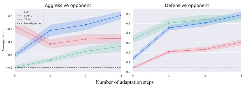
Under review as a conference paper at ICLR 2021

most applications. Second, most of these algorithms perform well only when the opponents during
testing are similar to the ones used for training, and it is difficult for them to adapt to opponents with
new styles quickly. More related works on opponent modeling are in Appendix A.1.
To overcome these shortcomings, we propose a novel Learning to Exploit (L2E) framework in this
work for implicit opponent modeling, which has two desirable advantages. First, L2E does not build
an explicit model for the opponent, so it does not require a large amount of interactive data and
eliminates the modeling errors simultaneously. Second, L2E can quickly adapt to new opponents
with unknown styles, with only a few interactions with them. The key idea underlying L2E to train a
base policy against various styles of opponents by using only a few interactions between them during
training, such that it acquires the ability to exploit different opponents quickly. After training, the
base policy can quickly adapt to new opponents using only a few interactions during testing. In
effect, our L2E framework optimizes for a base policy that is easy and fast to adapt. It can be seen
as a particular case of learning to learn, i.e., meta-learning (Finn et al., 2017). The meta-learning
algorithm (c.f ., Appendix A.2 for details), such as MAML (Finn et al., 2017), is initially designed
for single-agent environments. It requires manual design of training tasks, and the final performance
largely depends on the user-specified training task distribution. The L2E framework is designed
explicitly for the multi-agent competitive environments, which generates effective training tasks
(opponents) automatically (c.f ., Appendix A.3 for details). Some recent works have also initially
used meta-learning for opponent modeling. Unlike these works, which either use meta-learning to
predict the opponent’s behaviors (Rabinowitz et al., 2018) or to handle the non-stationarity problem
in multi-agent reinforcement learning (Al-Shedivat et al., 2018), we focus on how to improve the
agent’s ability to adapt to unknown opponents quickly.
In our L2E framework, the base policy is explicitly trained such that a few interactions with a
new opponent will produce an opponent-specific policy to effectively exploit this opponent, i.e.,
the base policy has strong adaptability that is broadly adaptive to many opponents. In specific, if
a deep neural network models the base policy, then the opponent-specific policy can be obtained
by fine-tuning the parameters of the base policy’s network using the new interactive data with the
opponent. A critical step in L2E is how to generate effective opponents to train the base policy.
The ideal training opponents should satisfy the following two desiderata. 1) The opponents need to
be challenging enough (i.e., hard to exploit). By learning to exploit these challenging opponents,
the base policy eliminates its weakness and learns a more robust strategy. 2) The opponents need
to have enough diversity. The more diverse the opponents during training, the stronger the base
policy’s generalization ability is, and the more adaptable the base policy to the new opponents.
To this end, we propose a novel opponent strategy generation (OSG) algorithm, which can produce
challenging and diverse opponents automatically. We use the idea of adversarial training to gener-
ate challenging opponents. Some previous works have also been proposed to obtain more robust
policies through adversarial training and showed that it improves the generalization (Pinto et al.,
2017; Pattanaik et al., 2018). From the perspective of the base policy, giving an opponent, the base
policy first adjusts itself to obtain an adapted policy, the base policy is then optimized to maximize
the rewards that the adapted policy gets when facing the opponent. The challenging opponents are
then adversarially generated by minimizing the base policy’s adaptability by automatically generat-
ing difficult to exploit opponents. These hard-to-exploit opponents are trained such that even if the
base policy adapts to them, the adapted base policy cannot take advantage of them. Besides, our
OSG algorithm can further produce diverse training opponents with a novel diversity-regularized
policy optimization procedure. In specific, we use the Maximum Mean Discrepancy (MMD) met-
ric (Gretton et al., 2007) to evaluate the differences between policies. The MMD metric is then
incorporated as a regularization term into the policy optimization process to obtain a diverse set of
opponent policies. By training with these challenging and diverse training opponents, the robustness
and generalization ability of our L2E framework can be significantly improved. To summarize, the
main contributions of this work are listed bellow in four-fold:

      • We propose a novel learning to exploit (L2E) framework to exploit sub-optimal opponents
        without building explicit models for it. L2E can quickly adapt to a new opponent with
        unknown style using only a few interactions.
      • We propose to use an adversarial training procedure to generate challenging opponents au-
        tomatically. These hard to exploit opponents help L2E eliminate its weakness and improve
        its robustness effectively.

                                                    2
Under review as a conference paper at ICLR 2021

Figure 1: The overview of our proposed L2E framework. The entire training process is based on
the idea of adversarial learning (Alg. 1). The base policy training part maximizes the base policy’s
adaptability by continually interacting with opponents of different strengths and styles (Section 2.1).
The opponent strategy generation part first generates hard-to-exploit opponents for the current base
policy (Hard-OSG, see Section 2.2.1), then generates diverse opponent policies to improve the gen-
eralization ability of the base policy (Diverse-OSG, see Section 2.2.2). The resulting base policy
can fast adapt to completely new opponents with a few interactions.

      • We further propose a diversity-regularized policy optimization procedure to generate di-
        verse opponents automatically. The generalization ability of L2E is improved significantly
        by training with these diverse opponents.
      • We conduct detailed experiments to evaluate the L2E framework in three different environ-
        ments. The experimental results demonstrate that the base policy trained with L2E quickly
        exploits a wide range of opponents compared to other algorithms.

2   M ETHOD

In this paper, we propose a novel L2E framework to endow the agents to adapt to diverse opponents
quickly. As shown in Fig. 1, L2E mainly consists of two modules, i.e., the base policy training part,
and the opponent strategy generation part. In the base policy training part, our goal is to find a base
policy that, given the unknown opponent, can fast adapt to it by using only a few interactions. To
this end, the base policy is trained to be able to adapt to many opponents. In specific, giving an
opponent O, the base policy B first adjusts itself to obtain an adapted policy B 0 by using a little
interaction data between O and B, the base policy is then optimized to maximize the rewards that
B 0 gets when facing O. In other words, the base policy has learned how to adapt to its opponents
and exploit them quickly.
The opponent strategy generation provides the base policy training part with challenging and diverse
training opponents automatically. First, our proposed opponent strategy generation (OSG) algorithm
can produce difficult to exploit opponents. In specific, the base policy B first adjusts itself to obtain
an adapted policy B 0 by using a little interaction data between O and B, the opponent O is then
optimized to minimize the rewards that B 0 gets when facing O. The resulting opponent O is hard to
exploit since even if the base policy B adapts to O, the adapted policy B 0 can not take advantage of
O. By training with these hard to exploit opponents, the base policy can eliminate its weakness and
improve its robustness effectively. Second, our OSG algorithm can further produce diverse training
opponents with a novel diversity-regularized policy optimization procedure. More specifically, we

                                                   3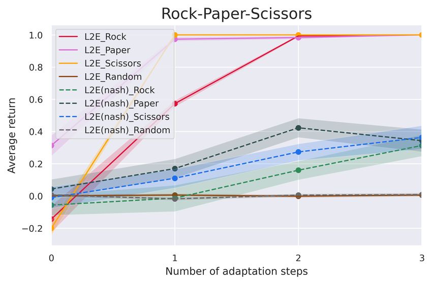
Under review as a conference paper at ICLR 2021

first formalize the difference between opponent policies as the difference between the distribution
of trajectories induced by each policy. The difference between distributions can be evaluated by
the Maximum Mean Discrepancy (MMD) metric (Gretton et al., 2007). Then, MMD is integrated
as a regularization term in the policy optimization process to identify various opponent policies.
By training with these diverse opponents, the base policy can improve its generalization ability
significantly. Next, we introduce these two modules in detail.

2.1   BASE P OLICY T RAINING

Our goal is to find a base policy B that can fast adapt to an unknown opponent O by updating
the parameters of B using only a few interactions between B and O. The key idea is to train
the base policy B against many opponents to maximize its payoffs by using only a small amount
of interactive data during training, such that it acquires the ability to exploit different opponents
quickly. In effect, our L2E framework treats each opponent as a training example. After training,
the resulting base policy B can quickly adapt to new and unknown opponents using only a few
interactions. Without loss of generality, the base policy B is modeled by a deep neural network
in this work, i.e., a parameterized function πθ with parameters θ. Similarly, the opponent O for
training is also a deep neural network πφ with parameters φ. We model the base policy as playing
against an opponent in a two-player Markov game (Shapley, 1953). This Markov game M =
(S, (AB , AO ), T, (RB , RO )) consists of the state space S, the action space AB and AO , and a state
transition function T : S × AB × AO → ∆ (S) where ∆ (S) is a probability distribution on S.
The reward function Ri : S × AB × AO × S → R for each player i ∈ {B, O} depends on the
current state, the next state and both players’ actions. Given a training opponent O whose policy
is known and fixed, this two-player Markov game M reduces to a single-player Markov Decision
Process (MDP), i.e., MBO = (S, AB , TBO , RB  O
                                                ). The state and action space of MBO are the same as in
M . The transition and reward functions have the opponent policy embedded:
                  TBO (s, aB ) = T (s, aB , aO ),    O
                                                    RB (s, aB , s0 ) = RB (s, aB , aO , s0 ),
                                                                                                   Y
where the opponent’s action is sampled from its policy aO ∼ πφ (· | s). Throughout the paper, MX
represents a single-player MDP, which is reduced from a two-player Markov game (i.e., player X
and player Y ). In this MDP, the player Y is fixed and can be regarded as part of the environment.
                                                                                               Oi
Suppose a set of training opponents {Oi }N
                                         i=1 is given. For each training opponent Oi , an MDP MB
can be constructed as described above. The base policy B, i.e., πθ is allowed to query a limited
number of sample trajectories τ to adapt to Oi . In our method, the adapted parameters θOi of the
base policy are computed using one or more gradient descent updates with the sample trajectories
τ . For example, when using one gradient update:
                                     θOi = θ − α∇θ LO  B (πθ ),
                                                        i
                                                                                                          (1)
                                                       Oi (t) (t) (t+1)
                                                X
                         LO
                          B (πθ ) = −Eτ ∼M Oi [
                            i
                                                  γ t RB  (s , aB , s   )].                               (2)
                                               B        t
                                                              (1)                  (t)
τ ∼ MBOi represents that the trajectory τ = {s(1) , aB , s(2) , . . . , s(t) , aB , s(t+1) , . . .} is sampled
                                                 (t)      (t)
from the MDP MBOi , where s(t+1) ∼ TBOi (s(t) , aB ) and aB ∼ πθ (· | s(t) ).
We use B Oi to denote the updated base policy, i.e., πθOi . B Oi can be seen as an opponent-specific
policy, which is updated from the base policy through fast adaptation. Our goal is to find a gener-
alizable base policy whose opponent-specific policy B Oi can exploit its opponent Oi as much as
possible. To this end, we optimize the parameters θ of the base policy to maximize the rewards that
B Oi gets when interacting with Oi . More concretely, the learning to exploit objective function is
defined as follows:
                       XN                           XN
                   min        LO i
                                 O
                                B i
                                    (π θ Oi ) = min        LO i
                                                             B Oi
                                                                  (πθ−α∇ LOi (π ) ).            (3)
                     θ       i=1                    θ         i=1              θ    B    θ

It is worth noting that the optimization is performed over the base policy’s parameters θ, whereas
the objective is computed using the adapted based policy’s parameters θOi . The parameters θ of the
base policy are updated as follows:
                                                XN
                                 θ = θ − β∇θ          LO i
                                                       B Oi
                                                            (πθOi ).                            (4)
                                                        i=1

                                                        4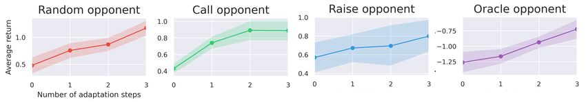
Under review as a conference paper at ICLR 2021

In effect, our L2E framework aims to find a base policy that can significantly exploit the opponent
with only a few interactions with it (i.e., with a few gradient steps). The resulting base policy has
learned how to adapt to different opponents and exploit them quickly. An overall description of the
base policy training procedure is shown in Alg. 1. The algorithm consists of three main steps. First,
generating hard to exploit opponents through the Hard-OSG module. Second, generating diverse
opponent policies through the Diverse-OSG module. Third, training the base policy with these
opponents to obtain fast adaptability.

2.2     AUTOMATIC O PPONENT G ENERATION

Previously, we assumed that the set of opponents had been given. How to automatically gener-
ate effective opponents for training is the key to the success of our L2E framework. The training
opponents should be challenging enough (i.e., hard to exploit). By learning to exploit these hard-to-
exploit opponents, the base policy B can eliminate its weakness and become more robust. Besides,
they should be sufficiently diverse. The more diverse they are, the stronger the generalization ability
of the resulting base policy. We propose a novel opponent strategy generation (OSG) algorithm to
achieve these goals.

2.2.1    H ARD - TO -E XPLOIT O PPONENTS G ENERATION
We use the idea of adversarial learning to generate challenging training opponents for the base
policy B. From the perspective of the base policy B, giving an opponent O, B first adjusts itself
to obtain an adapted policy, i.e., the opponent-specific policy B O , the base policy is then optimized
to maximize the rewards that B O gets when interacting with O. Contrary to the base policy’s goal,
we want to find a hard-to-exploit opponent O    b for the current base policy B, such that even if B
                                    O
adapts to O,
           b the adapted policy B cannot take advantage of O.    b In other words, the hard-to-exploit
                                     b

                                                           O
opponent O is trained to minimize the rewards that B gets when interacting with O.         b The base
           b                                               b

policy attempts to increase its adaptability by learning to exploit different opponents, while the hard-
to-exploit opponent adversarially tries to minimize the base policy’s adaptability, i.e., maximize its
counter-adaptability.
More concretely, the hard-to-exploit opponent O    b is also a deep neural network π b with randomly
                                                                                     φ
                       b At each training iteration, an MDP M Ob can be constructed. The base policy
initialized parameters φ.                                        B
                                                            b The parameters θOb of the adapted policy
B first query a limited number of trajectories to adapt to O.
B O are computed using one gradient descent update,
  b

                                    θO = θ − α∇θ LO B (πθ ).                                        (5)
                                         b                 b

                                                    b (t) (t) (t+1)
                                             X
                        LO
                         B (πθ ) = −Eτ ∼M O
                                          b[
                                                    O
                                               γ t RB (s , aB , s   )].                             (6)
                         b
                                             B     t

The parameters φb of O b is optimized to minimize the rewards that B Ob gets when interacting with
O.
 b This is equivalent to maximize the rewards that O b gets since we only consider the competitive
setting in this work. More concretely, the parameters φb are updated as follows:
                                                     O
                                  φb = φb − α∇φbLB
                                                           b

                                                   Ob (πφb)                                         (7)
                       BO                            B O (t) (t) (t+1)
                                             X
                                                γ t RO
                         b                             b
                      LO   b) = −E 0
                       b (πφ            BO
                                          b [         b (s , aO
                                                              b ,s     )].                          (8)
                                       τ ∼M b          t
                                             O

After several rounds of iteration, we can obtain a hard-to-exploit opponent πφb for the current base
policy B. An overall description of this procedure is shown in Alg. 2.

2.2.2    D IVERSE O PPONENTS G ENERATION
Training an effective base policy requires not only the hard-to-exploit opponents, but also diverse
opponents of different styles. The more diverse the opponents used for training, the stronger the
generalization ability of the resulting base policy. From a human player’s perspective, the opponent
style is usually defined as different types, such as aggressive, defensive, elusive, etc. The most sig-
nificant difference between opponents with different styles lies in the actions taken in the same state.

                                                   5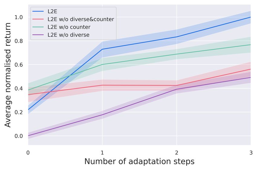
Under review as a conference paper at ICLR 2021

Take poker as an example; different opponents’ styles tend to take different actions when holding
the same hand. Based on the above analysis, we formalize the difference between opponent policies
as the difference between the distribution of trajectories induced by each policy when interacting
with the base policy. We argue that differences in trajectories better capture the differences between
different opponent policies.
Formally, given a base policy B, i.e., πθ and an opponent policy Oi , i.e., πφi , our diversity-
regularized policy optimization algorithm is to generate a new opponent Oj , i.e., πφj whose style
is different from Oi . We first construct two MDPs, i.e., MOBi and MOBj , and then sample two sets
of trajectories, i.e., Ti = {τ ∼ MOBi } and Tj = {τ ∼ MOBj } from this two MDPs. The stochas-
ticity in the MDP and the policy will induce a distribution over trajectories. We use the Maximum
Mean Discrepancy (MMD) (Gretton et al., 2007) metric (c.f . Appendix C for details) to measure the
differences between Ti and Tj :
    MMD2 (Ti , Tj ) = Eτ,τ 0 ∼MOB k (τ, τ 0 ) − 2Eτ ∼MOB ,τ 0 ∼MOB k(τ, τ 0 ) + Eτ,τ 0 ∼MOB k (τ, τ 0 ) .    (9)
                                         i                    i        j                     j

k is the Gaussian radial basis function kernel defined over a pair of trajectories:
                                                          kg(τ ) − g(τ 0 )k2
                                     k(τ, τ 0 ) = exp(−                      ),                             (10)
                                                                  2
where g stacks the states and actions of a trajectory into a vector. For trajectories with different
length, we clip the long trajectory to the same length as the short one. There overall objective
function of our proposed diversity-regularized policy optimization algorithm is as follows:
                                                        (t)
                                 X
          Lφi (φj ) = −Eτ ∼MOB [      γ t RO
                                           B
                                             j
                                               (s(t) , aOj , s(t+1) )] − αmmd MMD2 (Ti , Tj ).  (11)
                                     j           t

The first term is to maximize the rewards that Oj gets when interacting with the base policy B. The
second term measures the difference between Oj and the existing opponent Oi . By this diversity-
regularized policy optimization, the resulting opponent Oj is not only useful in performance but also
diverse relative to the existing policy.
We can iteratively apply the above algorithm to find a set of N distinct and diverse opponents.
In specific, subsequent opponents are learned by encouraging diversity with respect to previously
generated opponent set S. The distance between an opponent Om and an opponent set S is defined
by the distance between Om and On , where On ∈ S is the most similar policy to Om . Suppose we
have obtained a set of opponents S = {Om }M   m=1 , M < N . The M + 1-th opponent, i.e., πφM +1
can be obtained by optimizing:
                                                        (t)
                                X
  LS (φM +1 ) = −Eτ ∼MOB      [    γ t RO
                                        B
                                          M +1
                                               (s(t) , aOM +1 , s(t+1) )] − min MMD2 (Ti , TM +1 ).
                              M +1           t                                    Oi ∈S
                                                                                            (12)
By doing so, the resulting M + 1-th opponent remains diverse relative to the opponent set S. An
overall description of this procedure is shown in Alg. 3.

3     E XPERIMENTS
In this section, we conduct extensive experiments to evaluate the proposed L2E framework. We
evaluate algorithm performance on the Leduc poker, the BigLeduc poker and a Grid Soccer envi-
ronment, which are the commonly used benchmark for opponent modeling (Lanctot et al., 2017;
Steinberger, 2019; He et al., 2016). We first verify the trained base policy using our L2E framework
can fast exploit a wide range of opponents with only a few gradient updates. Then, we compare with
other baseline methods to show the superiority of our L2E framework. Finally, we conduct a series
of ablation experiments to demonstrate each part of our L2E framework’s effectiveness.

3.1    R APID A DAPTABILITY

In this section, we verify the trained base policy’s ability to quickly adapt to different opponents
in the Leduc poker environment (c.f . Appendix D for details). We provide four opponents with
different styles and strengths. 1) The random opponent randomly takes actions whose strategy is

                                                       6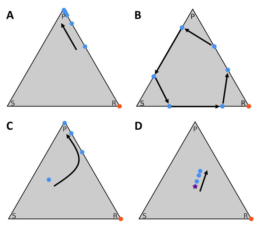
Under review as a conference paper at ICLR 2021

relatively weak but hard to exploit since it does not have an evident decision-making style. 2) The
call opponent always takes call actions and has a fixed decision-making style that is easy to exploit.
3) The rocks opponent takes actions based on its hand-strength whose strategy is relatively strong.
4) The oracle opponent is a cheating, and the strongest player who can see the other players’ hands
and make decisions based on this perfect information. As shown in Fig. 2, the base policy achieves a

Figure 2: The trained base policy using our L2E framework can quickly adapt to different opponents
of different styles and strengths in the Leduc poker environment.

rapid increase in its average returns with a few gradient updates against all four opponent strategies.
For the call opponent, which has a clear and monotonous style, the base policy can significantly
exploit it. Against the random opponent with no clear style, the base policy can also exploit it
quickly. When facing the strong rocks opponent or even the strongest oracle opponent, the base
policy can quickly improve its average returns. One significant advantage of the proposed L2E
framework is that the same base policy can exploit a wide range of opponents with different styles,
demonstrating its strong generalization ability.

3.2   C OMPARISONS WITH OTHER BASELINE M ETHODS

                                                Random          Call       Rocks        Nash         Oracle
                          L2E                   0.42±0.32   1.34±0.14    0.38±0.17    -0.03±0.14   -1.15±0.27
                        MAML                    1.27±0.17   -0.23±0.22   -1.42±0.07   -0.77±0.23   -2.93±0.17
                        Random                 -0.02±3.77   -0.02±3.31   -0.68±3.75   -0.74±4.26   -1.90±4.78
                         TRPO                   0.07±0.08   -0.22±0.09   -0.77±0.12   -0.42±0.07   -1.96±0.46
                  TRPO (pretrained)             0.15±0.17   -0.05±0.14   -0.70±0.27   -0.61±0.32   -1.32±0.27
            EOM (Explicit Opponent Modeling)    0.30±0.15   -0.01±0.05   -0.13±0.20   -0.36±0.11   -1.82±0.28

Table 1: The average return of each method when performing rapid adaptation against different
opponents in the Leduc Poker environment. The adaptation process is restricted to a three-step
gradient update.

As discussed in Section 1, most previous opponent modeling methods require constructing explicit
opponent models from a large amount of data before learning to adapt to new opponents. To the best
of our knowledge, our L2E framework is the first attempt to use meta-learning to learn to exploit
opponents without building explicit opponent models. To demonstrate the effectiveness of the L2E
framework, we design several competitive baseline methods. As with the previous experiments,
we also use three gradient updates when adapting to a new opponent. 1) MAML. The seminal
meta-learning algorithm MAML (Finn et al., 2017) is designed for single-agent environments. We
have redesigned and reimplemented the MAML algorithm for the two-player competitive environ-
ments. The MAML baseline trains a base policy by continually sampling the opponent’s strategies,
either manually specified or randomly generated. 2) TRPO. The TRPO baseline does not perform
pre-training and uses the TRPO algorithm (Schulman et al., 2015) to updated its parameters via
three-step gradient updates to adapt to different opponents. 3) Random. The Random baseline is
neither pre-trained nor updated online. To evaluate different algorithms more comprehensively, we
additionally add a new Nash opponent. This opponent’s policy is a part of an approximate Nash
Equilibrium generated iteratively by the CFR (Zinkevich et al., 2008) algorithm. Playing a strategy
from a Nash Equilibrium in a two-player zero-sum game is guaranteed not to lose in expectation
even if the opponent is the best response strategy when the value of the game is zero. We show
the performance of the various algorithms in Table 1. It is clear that L2E maintains the highest
profitability against all four types of opponents other than the random type. L2E can exploit the
opponent with evident style significantly, such as the the Call opponent. Compared to other baseline
methods, L2E achieved the highest average return against opponents with unclear styles, such as the
Rocks opponent, the Nash opponent, and the cheating Oracle opponent.

                                                            7
Under review as a conference paper at ICLR 2021
3.3 A BLATION S TUDIES
3.3.1 E FFECTS OF THE D IVERSITY- REGULARIZED P OLICY O PTIMIZATION
Figure 3: Visualization of the styles of the strategies generated with or without the MMD regular-
ization term in the Leduc poker environment.
In this section, we verify whether our proposed diversity-regularized policy optimization algorithm
can effectively generate policies with different styles. In Leduc poker, hand-action pairs represent
different combinations of hands and actions. In the pre-flop phase, each player’s hand has three
possibilities, i.e., J, Q, and K. Meanwhile, each player also has three optional actions, i.e., Call (c),
Rise (r), and Fold (f). For example, ‘Jc’ means to call when getting the jack. Action probability is the
probability that a player will take a corresponding action with a particular hand. Fig. 3 demonstrates
that without the MMD regularization term, the two sets of strategies generated in both the pre-flop
and flop phases have similar styles. By optimizing with the MMD regularization term, the generated
strategies are diverse enough which cover a wide range of different states and actions.
3.3.2 E FFECTS OF THE H ARD -OSG AND THE D IVERSE -OSG
As discussed previously, a crucial step in L2E is the
automatic generation of training opponents. The Hard-
OSG and Diverse-OSG modules are used to gener-
ate opponents that are difficult to exploit and diverse
in styles. Fig. 4 shows the impact of each mod-
ule on the performance of L2E. ‘L2E w/o counter’ is
L2E without the Hard-OSG module. Similarly, ‘L2E
w/o diverse’ is L2E without the Diverse-OSG module.
‘L2E w/o diverse&counter’ removes both modules al-
together. The results show that both Hard-OSG and
Diverse-OSG have a crucial influence on L2E’s per-
formance. It is clear that the Hard-OSG module helps
to enhance the stability of the base policy, and the Figure 4: Each curve shows the aver-
Diverse-OSG module can improve the base policy’s age normalized returns of the base policy
performance significantly. To further demonstrate the trained with different variants of L2E in the
generalization ability of L2E, we conducted a series of grid soccer environment.
additional experiments on the BigLeduc poker and a
Grid Soccer game environment (c.f . Appendix E and Appendix F for details).
4 C ONCLUSION
We propose a learning to exploit (L2E) framework to exploit sub-optimal opponents without build-
ing explicit opponent models. L2E acquires the ability to exploit opponents by a few interactions
with different opponents during training, so that it adapts to new opponents during testing quickly.
We propose a novel opponent strategy generation algorithm that produces effective training oppo-
nents for L2E automatically. We first design an adversarial training procedure to generate challeng-
ing opponents to improve L2E’s robustness effectively. We further exploit a diversity-regularized
policy optimization procedure to generate diverse opponents to improve L2E’s generalization abil-
ity significantly. Detailed experimental results in three challenging environments demonstrate the
effectiveness of the proposed L2E framework.
8Under review as a conference paper at ICLR 2021
R EFERENCES
Mohammed Amin Abdullah, Hang Ren, Haitham Bou Ammar, Vladimir Milenkovic, Rui Luo,
Mingtian Zhang, and Jun Wang. Wasserstein robust reinforcement learning. arXiv preprint
arXiv:1907.13196, 2019.
Alexandros Agapitos, Julian Togelius, Simon M Lucas, Jurgen Schmidhuber, and Andreas Konstan-
tinidis. Generating diverse opponents with multiobjective evolution. In IEEE Symposium On
Computational Intelligence and Games, pp. 135–142, 2008.
Maruan Al-Shedivat, Trapit Bansal, Yura Burda, Ilya Sutskever, Igor Mordatch, and Pieter Abbeel.
Continuous adaptation via meta-learning in nonstationary and competitive environments. In In-
ternational Conference on Learning Representations, 2018.
Stefano V Albrecht and Peter Stone. Reasoning about hypothetical agent behaviours and their pa-
rameters. In International Conference on Autonomous Agents and Multiagent Systems, pp. 547–
555, 2017.
Stefano V Albrecht and Peter Stone. Autonomous agents modelling other agents: A comprehensive
survey and open problems. Artificial Intelligence, 258:66–95, 2018.
Dipyaman Banerjee and Sandip Sen. Reaching pareto-optimality in prisoner’s dilemma using con-
ditional joint action learning. Autonomous Agents and Multi-Agent Systems, 15(1):91–108, 2007.
George W Brown. Iterative solution of games by fictitious play. Activity analysis of production and
allocation, 13(1):374–376, 1951.
Harmen de Weerd, Rineke Verbrugge, and Bart Verheij. Negotiating with other minds: the role of
recursive theory of mind in negotiation with incomplete information. Autonomous Agents and
Multi-Agent Systems, 31(2):250–287, 2017.
Eddie Dekel, Drew Fudenberg, and David K Levine. Learning to play bayesian games. Games and
Economic Behavior, 46(2):282–303, 2004.
Benjamin Eysenbach, Abhishek Gupta, Julian Ibarz, and Sergey Levine. Diversity is all you need:
Learning skills without a reward function. In International Conference on Learning Representa-
tions, 2018.
Chelsea Finn, Pieter Abbeel, and Sergey Levine. Model-agnostic meta-learning for fast adaptation
of deep networks. In International Conference on Machine Learning, pp. 1126–1135, 2017.
Jakob Foerster, Richard Y Chen, Maruan Al-Shedivat, Shimon Whiteson, Pieter Abbeel, and Igor
Mordatch. Learning with opponent-learning awareness. In International Conference on Au-
tonomous Agents and MultiAgent Systems, pp. 122–130, 2018.
Meire Fortunato, Mohammad Gheshlaghi Azar, Bilal Piot, Jacob Menick, Matteo Hessel, Ian Os-
band, Alex Graves, Volodymyr Mnih, Remi Munos, Demis Hassabis, et al. Noisy networks for
exploration. In International Conference on Learning Representations, 2018.
Arthur Gretton, Karsten Borgwardt, Malte Rasch, Bernhard Schölkopf, and Alex J Smola. A kernel
method for the two-sample-problem. In Advances in neural information processing systems, pp.
513–520, 2007.
Barbara Grosz and Candace L Sidner. Attention, intentions, and the structure of discourse. Compu-
tational linguistics, 1986.
Abhishek Gupta, Benjamin Eysenbach, Chelsea Finn, and Sergey Levine. Unsupervised meta-
learning for reinforcement learning. arXiv preprint arXiv:1806.04640, 2018.
He He, Jordan Boyd-Graber, Kevin Kwok, and Hal Daumé III. Opponent modeling in deep rein-
forcement learning. In International conference on machine learning, pp. 1804–1813, 2016.
Timothy Hospedales, Antreas Antoniou, Paul Micaelli, and Amos Storkey. Meta-learning in neural
networks: A survey. arXiv preprint arXiv:2004.05439, 2020.
9Under review as a conference paper at ICLR 2021
Trung Dong Huynh, Nicholas R Jennings, and Nigel R Shadbolt. An integrated trust and reputation
model for open multi-agent systems. Autonomous Agents and Multi-Agent Systems, 13(2):119–
154, 2006.
Max Jaderberg, Valentin Dalibard, Simon Osindero, Wojciech M Czarnecki, Jeff Donahue, Ali
Razavi, Oriol Vinyals, Tim Green, Iain Dunning, Karen Simonyan, et al. Population based train-
ing of neural networks. arXiv preprint arXiv:1711.09846, 2017.
Max Jaderberg, Wojciech M Czarnecki, Iain Dunning, Luke Marris, Guy Lever, Antonio Garcia
Castaneda, Charles Beattie, Neil C Rabinowitz, Ari S Morcos, Avraham Ruderman, et al. Human-
level performance in 3d multiplayer games with population-based reinforcement learning. Sci-
ence, 364(6443):859–865, 2019.
Peter A Jarvis, Teresa F Lunt, and Karen L Myers. Identifying terrorist activity with ai plan recog-
nition technology. AI magazine, 26(3):73–73, 2005.
Marc Lanctot, Vinicius Zambaldi, Audrunas Gruslys, Angeliki Lazaridou, Karl Tuyls, Julien
Pérolat, David Silver, and Thore Graepel. A unified game-theoretic approach to multiagent re-
inforcement learning. In Advances in neural information processing systems, pp. 4190–4203,
2017.
Gordon McCalla, Julita Vassileva, Jim Greer, and Susan Bull. Active learner modelling. In Interna-
tional Conference on Intelligent Tutoring Systems, pp. 53–62, 2000.
Richard Mealing and Jonathan L Shapiro. Opponent modeling by expectation–maximization and
sequence prediction in simplified poker. IEEE Transactions on Computational Intelligence and
AI in Games, 9(1):11–24, 2015.
Christian Muise, Vaishak Belle, Paolo Felli, Sheila McIlraith, Tim Miller, Adrian R Pearce, and Liz
Sonenberg. Planning over multi-agent epistemic states: A classical planning approach. In AAAI
Conference on Artificial Intelligence, 2015.
John H Nachbar. Beliefs in repeated games. Econometrica, 73(2):459–480, 2005.
Alex Nichol, Joshua Achiam, and John Schulman. On first-order meta-learning algorithms. arXiv
preprint arXiv:1803.02999, 2018.
Anay Pattanaik, Zhenyi Tang, Shuijing Liu, Gautham Bommannan, and Girish Chowdhary. Robust
deep reinforcement learning with adversarial attacks. In International Conference on Autonomous
Agents and MultiAgent Systems, pp. 2040–2042, 2018.
Lerrel Pinto, James Davidson, Rahul Sukthankar, and Abhinav Gupta. Robust adversarial reinforce-
ment learning. In International Conference on Machine Learning, pp. 2817–2826, 2017.
Matthias Plappert, Rein Houthooft, Prafulla Dhariwal, Szymon Sidor, Richard Y Chen, Xi Chen,
Tamim Asfour, Pieter Abbeel, and Marcin Andrychowicz. Parameter space noise for exploration.
In International Conference on Learning Representations, 2018.
Rob Powers and Yoav Shoham. Learning against opponents with bounded memory. In International
joint conference on Artificial intelligence, pp. 817–822, 2005.
Neil Rabinowitz, Frank Perbet, Francis Song, Chiyuan Zhang, SM Ali Eslami, and Matthew
Botvinick. Machine theory of mind. In International Conference on Machine Learning, pp.
4218–4227, 2018.
John Schulman, Sergey Levine, Pieter Abbeel, Michael Jordan, and Philipp Moritz. Trust region
policy optimization. In International conference on machine learning, pp. 1889–1897, 2015.
Lloyd S Shapley. Stochastic games. Proceedings of the national academy of sciences, 39(10):
1095–1100, 1953.
Eric Steinberger. Single deep counterfactual regret minimization. arXiv preprint arXiv:1901.07621,
2019.
10Under review as a conference paper at ICLR 2021
Gita Sukthankar and Katia Sycara. Policy recognition for multi-player tactical scenarios. In Inter-
national joint conference on Autonomous agents and multiagent systems, pp. 1–8, 2007.
Gabriel Synnaeve and Pierre Bessiere. A bayesian model for opening prediction in rts games with
application to starcraft. In IEEE Conference on Computational Intelligence and Games, pp. 281–
288, 2011.
Oriol Vinyals, Igor Babuschkin, Wojciech M Czarnecki, Michaël Mathieu, Andrew Dudzik, Juny-
oung Chung, David H Choi, Richard Powell, Timo Ewalds, Petko Georgiev, et al. Grandmaster
level in starcraft ii using multi-agent reinforcement learning. Nature, 575(7782):350–354, 2019.
Jane X Wang, Zeb Kurth-Nelson, Dhruva Tirumala, Hubert Soyer, Joel Z Leibo, Remi Munos,
Charles Blundell, Dharshan Kumaran, and Matt Botvinick. Learning to reinforcement learn.
arXiv preprint arXiv:1611.05763, 2016.
Rui Wang, Joel Lehman, Jeff Clune, and Kenneth O Stanley. Paired open-ended trailblazer (poet):
Endlessly generating increasingly complex and diverse learning environments and their solutions.
arXiv preprint arXiv:1901.01753, 2019.
Ben G Weber and Michael Mateas. A data mining approach to strategy prediction. In IEEE Sympo-
sium on Computational Intelligence and Games, pp. 140–147, 2009.
Ying Wen, Yaodong Yang, Rui Luo, Jun Wang, and Wei Pan. Probabilistic recursive reasoning for
multi-agent reinforcement learning. In International Conference on Learning Representations,
2018.
Zhongwen Xu, Hado P van Hasselt, and David Silver. Meta-gradient reinforcement learning. In
Advances in neural information processing systems, pp. 2396–2407, 2018.
Martin Zinkevich, Michael Johanson, Michael Bowling, and Carmelo Piccione. Regret minimization
in games with incomplete information. In Advances in neural information processing systems, pp.
1729–1736, 2008.
A R ELATED W ORK
A.1 O PPONENT M ODELING
Opponent modeling is a long-standing research topic in artificial intelligence, and some of the ear-
liest works go back to the early days of game theory research (Brown, 1951). The main goal of
opponent modeling is to interact more effectively with other agents by building models to reason
about their intentions, predicting their next moves or other properties (Albrecht & Stone, 2018).
The commonly used opponent modeling methods can be roughly divided into four categories: policy
reconstruction, classification, type-based reasoning and recursive reasoning. Policy reconstruction
methods (Mealing & Shapiro, 2015) reconstruct the opponents’ decision making process by build-
ing models which make explicit predictions about their actions. Classification methods (Weber &
Mateas, 2009; Synnaeve & Bessiere, 2011) produce models which assign class labels (e.g., “aggres-
sive” or “defensive”) to the opponent and employ a precomputed strategy which is effective against
that particular class of opponent. Type-based reasoning methods (He et al., 2016; Albrecht & Stone,
2017) assume that the opponent has one of several known types and update the belief using the new
observations obtained during the real-time interactions. Recursive reasoning based methods (Muise
et al., 2015; de Weerd et al., 2017) model the nested beliefs (e.g., “I believe that you believe that I
believe...”) and simulate the reasoning processes of the opponents to predict their actions. Different
from these existing methods which usually require a large amount of interactive data to generate
useful opponent models, our L2E framework does not explicitly model the opponent and acquires
the ability to exploit different opponents by training with limited interactions with different styles of
opponents.
11Under review as a conference paper at ICLR 2021
A.2 M ETA -L EARNING
Meta-learning is a new trend of research in the machine learning community which tackles the
problem of learning to learn (Hospedales et al., 2020). It leverages past experiences in the training
phase to learn how to learn, acquiring the ability to generalize to new environments or new tasks.
Recent progress in meta-learning has achieved impressive results ranging from classification and
regression in supervised learning (Finn et al., 2017; Nichol et al., 2018) to new task adaption in
reinforcement learning (Wang et al., 2016; Xu et al., 2018). Some recent works have also initially
explored the application of meta-learning in opponent modeling. For example, the theory of mind
network (ToMnet) (Rabinowitz et al., 2018) uses meta-learning to improve the predictions about the
opponents’ future behaviors. Another related work (Al-Shedivat et al., 2018) uses meta-learning to
handle the non-stationarity problem in the multi-agent interactions. Different from these methods,
we focus on how to improve the agents’ ability to quickly adapt to different and unknown opponents.
A.3 S TRATEGY G ENERATION
The automatic generation of effective opponent strategies for training with is a critical step in our
approach, and how to generate diverse strategies has been preliminarily studied in the reinforce-
ment learning community. In specific, diverse strategies can be obtained in a variety of ways, in-
cluding adding some diversity regularization to the optimization objective (Abdullah et al., 2019),
randomly searching in some diverse parameter space (Plappert et al., 2018; Fortunato et al., 2018),
using information-based strategy proposal (Eysenbach et al., 2018; Gupta et al., 2018) and search-
ing diverse strategies with evolutionary algorithms (Agapitos et al., 2008; Wang et al., 2019; Jader-
berg et al., 2017; 2019). More recently, the researchers from DeepMind propose a league training
paradigm to obtain a Grandmaster level StarCraft II AI (i.e., AlphaStar) by training a diverse league
of clorntinually adapting strategies and counter-strategies (Vinyals et al., 2019). Different from
AlphaStar, our opponent strategy generation algorithm exploits adversarial training and diversity-
regularized policy optimization to produce challenging and diverse opponents respectively.
B A LGORITHM
Algorithm 1: The base policy training procedure of our L2E framework.
Input: Step size hyper parameters α,β; base policy B with parameters θ; opponent policy O
with parameters φ.
Output: An adaptive base policy B with parameters θ
randomly initialize θ,φ ;
initialize policy pool M = {O} ;
for 1 < e ≤ epochs do
O = Hard-OSG(B) .(see Alg. 2 ) ;
P =Diverse-OSG(B, O, N ) .(see Alg. 3) ;
Update opponent policy pool M = M ∪ P ;
Sample batch of opponents Oi ∼ M ;
for Each opponent Oi do
Construct a single-player MDP MBOi ;
Sample trajectories τ using B against fixed opponent Oi ;
Use Eqn. (1) to update the parameters of B to obtain an adapted policy B Oi ;
Resample trajectories τ 0 using B Oi against Oi ;
Update the parameters θ of B according to Eqn. (4);
C M AXIMUM M EAN D ISCREPANCY
We use the Maximum Mean Difference (MMD) (Gretton et al., 2007) metric to measure the differ-
ences between the distributions of trajectories induced by different opponent strategies.
12Under review as a conference paper at ICLR 2021
Algorithm 2: Hard-OSG, the hard-to-exploit training opponent generation algorithm.
Input: The latest base policy B with parameters θ.
Output: A hard-to-exploit opponent O b for B.
Randomly initialize O’s parameters φ ;
b b
for 1 ≤ i ≤ epochs do
Construct a single-player MDP MBO ;
b
Sample a small number of trajectories τ ∼ MBO using B against O b;
b
Use Eqn. (5) to update the parameters of B to obtain an adapted policy B O ;
b
O
Sample trajectories τ 0 ∼ M B using O b against B Ob ;
b
O
b
Update the parameters φb of O
b according to Eqn. (7) ;
Algorithm 3: Diverse-OSG, the proposed diversity-regularized policy optimization algorithm to
generate diverse training opponents.
Input: The latest base policy B, an exsiting opponent O1 , the total number of opponents that to
be generated N .
Output: A set of diverse opponent S = {Om }N m=1
Initialize the opponent set S = {O1 } ;
for i = 2 to N do
Randonly initialize an opponent Oi ’s parameters φi ;
for 1 ≤ t ≤ steps do
Calculate the objective function LS (φi ) according to Eqn. (12);
Calucute the gradient ∇φi LS (φi ) (c.f ., Appendix C for details) ;
Use this gradient to update φi ;
Update the opponent set S, i.e., S = S ∪ Oi
Definition 1 Let F be a function space f : X → R. Suppose we have two distributions p and q,
X := {x1 , ..., xm } ∼ p, Y := {y1 , ..., yn } ∼ q. The MMD between p and q using test functions
from the function space F is defined as follows:
MMD[F, p, q] := sup (Ex∼p [f (x)] − Ey∼q [f (y)]) . (13)
f ∈F
If we can pick a suitable function space F, we get the following important theorem (Gretton et al.,
2007).
Theorem 1 Let F = {f | kf kH ≤ 1} be a unit ball in a Reproducing Kernel Hilbert Space (RKHS).
Then MMD[F, p, q] = 0 if and only if p = q.
So the MMD distance between two strategies is 0 when the distributions of trajectories induced by
them are identical. To obtain a set of strategies with diverse styles, we should increase the MMD
distances between different strategies. ϕ is a feature space mapping from x to RKHS, we can easily
Algorithm 4: The testing procedure of our L2E framework.
Input: Step size hyper parameters α; The trained base policy B with parameters θ; an
unknown opponent O.
Output: The updated base policy B O that has been adapted to the opponent O.
Construct a single-player MDP MBO ;
for 0 < step ≤ steps do
Sample trajectories τ from the MDP MBO ;
Update the parameters θ of B according to Eqn. (1);
13Under review as a conference paper at ICLR 2021
calculate the MMD distance using the kernel method k(x, x0 ) := hϕ(x), ϕ(x0 )iH :
MMD2 (F, p, q)
2
= kEX∼p ϕ(X) − EY ∼q ϕ(Y )kH
(14)
= hEX∼p ϕ(X) − EY ∼q ϕ(Y ), EX∼p ϕ(X) − EY ∼q ϕ(Y )i
=EX,X 0 ∼p k (X, X 0 ) − 2EX∼p,Y ∼q k(X, Y ) + EY,Y 0 ∼q k (Y, Y 0 ) .
The expectation terms in Eqn. (14) can be approximated using samples:
Pm
MMD2 [F, X, Y ] = m(m−1)1
i6=j k (xi , xj )
Pn Pm,n (15)
1 2
+ n(n−1) i6=j k (yi , yj ) − mn i,j=1 k (xi , yj ) .
The gradient of the MMD term with respect to the policy’s parameter φj in our L2E framework can
be calculated as follows:
∇φj MMD2 (Ti , Tj ) = ∇φj MMD2 ({τ ∼ MOBi }, {τ ∼ MOBj })
= Eτ,τ 0 ∼MOB [k (τ, τ 0 ) ∇φj log(p(τ )p(τ 0 ))]
i
(16)
− 2Eτ ∼MOB ,τ 0 ∼MOB [k (τ, τ 0 ) ∇φj log(p(τ )p(τ 0 ))]
i j
+ Eτ,τ 0 ∼MOB [k (τ, τ 0 ) ∇φj log(p(τ )p(τ 0 ))],
j
where p(τ ) is the probability of the trajectory. Since Ti = {τ ∼ MOBi }, Oi is the known opponent
policy that has no dependence on φj . The gradient with respect to the parameters φj in first term is
0. The gradient of the second and third terms can be easily calculated as follows:
XT
∇φj log(p(τ )) = ∇φj log πφj (at |st ). (17)
t=0
D L EDUC P OKER
The Leduc poker generally uses a deck of six cards that includes two suites, each with three ranks
(Jack, Queen, and King of Spades, Jack, Queen, and King of Hearts). The game has a total of
two rounds. Each player is dealt with a private card in the first round, with the opponent’s deck
information hidden. In the second round, another card is dealt with as a community card, and the
information about this card is open to both players. If a player’s private card is paired with the
community card, that player wins the game; otherwise, the player with the highest private card wins
the game. Both players bet one chip into the pot before the cards are dealt. Moreover, a betting
round follows at the end of each dealing round. The betting wheel alternates between two players,
where each player can choose between the following actions: call, check, raise, or fold. If a player
chooses to call, that player will need to increase his bet until both players have the same number
of chips. If one player raises, that player must first make up the chip difference and then place an
additional bet. Check means that a player does not choose any action on the round, but can only
check if both players have the same chips. If a player chooses to fold, the hand ends, and the other
player wins the game. When all players have equal chips for the round, the game moves on to the
next round. The final winner wins all the chips in the game.
Next, we introduce how to define the state vector. Position in a poker game is a critical piece
of information that determines the order of action. We define the button (the pre-flop first-hand
position), the action position (whose turn it is to take action), and the current game round as one
dimension of the state, respectively. In Poker, the combination of a player’s hole cards and board
cards determines the game’s outcome. We encode the hole cards and the board cards separately. The
amount of chips is an essential consideration in a player’s decision-making process. We encode this
information into two dimensions of the state. The number of chips in the pot can reflect the action
history of both players. The difference in bets between players in this round affects the choice of
action (the game goes to the next round until both players have the same number of chips). In
summary, the state vector has seven dimensions, i.e., button, to act, round, hole cards, board cards,
chips to call, and pot.
14Under review as a conference paper at ICLR 2021
E B IG L EDUC P OKER
We use a larger and more challenging BigLeduc poker environment to further verify the effectiveness
of our L2E framework. The BigLeduc poker has the same rules as Leduc but uses a deck of 24 cards
with 12 ranks. In addition to the larger state space, BigLeduc allows a maximum of 6 instead of 2
raises per round. As shown in Fig. 5, L2E still achieves fast adaptation to different opponents. In
comparison with other baseline methods, L2E achieves the highest average return in Table 2.
Random Call Raise Oracle
L2E 0.82±0.28 0.74±0.22 0.68±0.09 -1.02±0.24
MAML 0.77±0.30 0.17±0.08 -2.02±0.99 -1.21±0.30
Random -0.00±3.08 -0.00±2.78 -2.83±5.25 -1.88±4.28
TRPO 0.19±0.09 0.10±0.16 -2.22±0.71 -1.42±0.47
TRPO (pretrained) 0.36±0.42 0.23±0.21 -2.03±1.61 -1.69±0.69
EOM 0.56±0.43 0.15±0.13 -1.15±0.12 -1.63±0.62
Table 2: The average return of each method when performing rapid adaptation against different
opponents in the BigLeduc poker environment.
Figure 5: The trained base policy using our L2E framework can quickly adapt to different opponents
of different styles and strengths in the BigLeduc poker environment.
F G RID S OCCER
This game contains a board with a 6 × 9 grid, two players, and their respective target areas. The
position of the target area is fixed, and the two players appear randomly in their respective areas at
the start of the game. One of the two players randomly has the ball. The goal of all players is to
move the ball to the other player’s target position. When the two players move to the same grid, the
player with the ball loses the ball. Players gain one point for moving the ball to the opponent’s area.
The player can move in all four directions within the grid, and action is invalid when it moves to the
boundary.
We train the L2E algorithm in this soccer environment in which both players are modeled by a
neural network. Inputs to the network include information about the position of both players, the
position of the ball, and the boundary. We provide two types of opponents to test the effectiveness
of the resulting base policy. 1) A defensive opponent who adopts a strategy of not leaving the
target area and preventing opposing players from attacking. 2) An aggressive opponent who adopts
a strategy of continually stealing the ball and approaching the target area with the ball. Facing
a defensive opponent won’t lose points, but the agent must learn to carry the ball and avoid the
opponent moving to the target area to score points. Against an aggressive opponent, the agent must
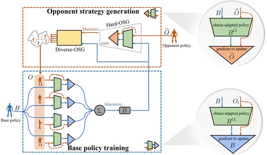
learn to defend at the target area to avoid losing points. Fig. 6 shows the comparisons between
L2E, MAML, and TRPO. L2E adapts quickly to both types of opponents; TRPO works well against
defensive opponents but loses many points against aggressive opponents; MAML is unstable due to
its reliance on task specification during the training process.
15Under review as a conference paper at ICLR 2021
Figure 6: The trained base policy using our L2E framework can quickly adapt to opponents with
different styles in a Grid Soccer environment.
G CONVERGENCE
Since convergence in game theory is difficult to analyze theoretically, we have designed a series of
small-scale experiments to empirically verify the convergence of L2E with the help of Rock-Paper-
Scissors(RPS) game. There are several reasons why RPS game is chosen: 1. RPS game is easy
to analyze due to the small state and action space. 2. RPS game is easy to visualize and analyze
due to the small state and action space. 3. RPS game is often used in game theory for theoretical
analysis. The experiments we designed contains the following parts: 1. Testing the adaptability of
Policy Gradient (PG), Self Play (SF), and L2E by visualizing the adaptation process. 2. Analyzing
the relationship between L2E strategy and Nash strategy. 3. Analyzing the convergence of L2E.
Figure 7: A. Policy Gradient : Optimize iteratively for the initial opponent (the orange dot), eventu-
ally converging to the best response of the initial opponent’s strategy. B. Self Play : Each iteration
seeks the best response to the previous round of strategy, which does not converge in an intransitive
game like RPS. C. L2E’s adaptation process when facing a new opponent (the orange dot). D. Nash
policy’s adaptation process when facing a new opponent (the orange dot).
As shown in Fig. 7, we can draw the following conclusions: 1. PG eventually converged to the best
response, but it took dozens of gradient descent steps in our experiments (Each blue dot represents
a ten-step gradient descent). SP failed to converge in the RPS game due to the intransitive nature of
the RPS game (Rock>Scissors>Paper>Rock). In contrast, our L2E quickly converged to the best
response strategy (Each blue dot represents a one-step gradient descent). 2. The strategy visualiza-
tion in the Fig. 7.C shows that the base policy of L2E does not converge to the Nash equilibrium
strategy after training but converges to the vicinity of the Nash equilibrium strategy. 3. If we fix
16You can also read