ElasticFusion: Dense SLAM Without A Pose Graph
←
→
Page content transcription
If your browser does not render page correctly, please read the page content below
ElasticFusion: Dense SLAM Without A Pose Graph
    Thomas Whelan*, Stefan Leutenegger*, Renato F. Salas-Moreno† , Ben Glocker† and Andrew J. Davison*
         *Dyson Robotics Laboratory at Imperial College, Department of Computing, Imperial College London, UK
                               †
                                 Department of Computing, Imperial College London, UK
                    {t.whelan,s.leutenegger,r.salas-moreno10,b.glocker,a.davison}@imperial.ac.uk

   Abstract—We present a novel approach to real-time dense
visual SLAM. Our system is capable of capturing comprehensive
dense globally consistent surfel-based maps of room scale envi-
ronments explored using an RGB-D camera in an incremental
online fashion, without pose graph optimisation or any post-
processing steps. This is accomplished by using dense frame-to-
model camera tracking and windowed surfel-based fusion cou-
pled with frequent model refinement through non-rigid surface
deformations. Our approach applies local model-to-model surface
loop closure optimisations as often as possible to stay close to the
mode of the map distribution, while utilising global loop closure
to recover from arbitrary drift and maintain global consistency.

                       I. I NTRODUCTION
                                                                       Fig. 1: Comprehensive scan of an office containing over 4.5
    In dense 3D SLAM, a space is mapped by fusing the data             million surfels captured in real-time.
from a moving sensor into a representation of the continuous
surfaces it contains, permitting accurate viewpoint-invariant
localisation as well as offering the potential for detailed            have relied on alternation and effectively per-surface-element-
semantic scene understanding. However, existing dense SLAM             independent filtering [15, 9]. However, it has been observed in
methods suitable for incremental, real-time operation struggle         the field of dense visual SLAM that the enormous weight of
when the sensor makes movements which are both of extended             data serves to overpower the approximations to joint filtering
duration and often criss-cross loop back on themselves. Such           which this assumes. This also raises the question as to whether
a trajectory is typical if a non-expert person with a handheld         it is optimal to attach a dense frontend to a sparse pose graph
depth camera were to scan in a room with a loopy “painting”            structure like its feature-based visual SLAM counterpart. Pose
motion; or would also be characteristic of a robot aiming to           graph SLAM systems primarily focus on optimising the cam-
explore and densely map an unknown environment.                        era trajectory, whereas our approach (utilising a deformation
    SLAM algorithms have too often targeted one of two ex-             graph) instead focuses on optimising the map.
tremes; (i) either extremely loopy motion in a very small area            Some examples of recent real-time dense visual SLAM
(e.g. MonoSLAM [4] or KinectFusion [15]) or (ii) “corridor-            systems that utilise pose graphs include that of Whelan et
like” motion on much larger scales but with fewer loop                 al. which parameterises a non-rigid surface deformation with
closures (e.g. McDonald et al. [13] or Whelan et al. [25]). In         an optimised pose graph to perform occasional loop closures
sparse feature-based SLAM, it is well understood that loopy            in corridor-like trajectories [25]. This approach is known to
local motion can be dealt with either via joint probabilistic          scale well but perform poorly given locally loopy trajectories
filtering [3], or in-the-loop joint optimisation of poses and          while being unable to re-use revisited areas of the map. The
features (bundle adjustment) [11]; and that large scale loop           DVO SLAM system of Kerl et al. applies keyframe-based
closures can be dealt with via partitioning of the map into            pose graph optimisation principles to a dense tracking frontend
local maps or keyframes and applying pose graph optimisation           but performs no explicit map reconstruction and functions off
[12]. In fact, even in sparse feature-based SLAM there have            of raw keyframes alone [10]. Meilland and Comport’s work
been relatively few attempts to deal with motion which is both         on unified keyframes utilises fused predicted 2.5D keyframes
extended and extremely loopy, such as Strasdat et al.’s work           of mapped environments while employing pose graph opti-
on double window optimisation [20].                                    misation to close large loops and align keyframes, although
    With a dense vision frontend, the number of points matched         not creating an explicit continuous 3D surface [14]. MRSMap
and measured at each sensor frame is much higher than                  by Stückler and Behnke registers octree encoded surfel maps
in feature-based systems (typically hundreds of thousands).            together for pose estimation. After pose graph optimisation the
This makes joint filtering or bundle adjustment local opti-            final map is created by merging key surfel views [21].
misation computationally infeasible. Instead, dense frontends             In our system we wish to move away from the focus on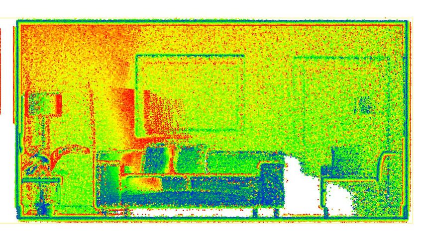
Fig. 2: Example SLAM sequence with active model coloured by surface normal overlaid on the inactive model in greyscale; (i)
Initially all data is in the active model as the camera moves left; (ii) As time goes on, the area of map not seen recently is set
to inactive. Note the highlighted area; (iii) The camera revisits the inactive area of the map, closing a local loop and registering
the surface together. The previously highlighted inactive region then becomes active; (iv) Camera exploration continues to the
right and more loops are closed; (v) Continued exploration to new areas; (vi) The camera revisits an inactive area but has
drifted too far for a local loop closure; (vii) Here the misalignment is apparent, with red arrows visualising equivalent points
from active to inactive; (viii) A global loop closure is triggered which aligns the active and inactive model; (ix) Exploration
to the right continues as more local loop closures are made and inactive areas reactivated; (x) Final full map coloured with
surface normals showing underlying deformation graph and sampled camera poses in global loop closure database.

pose graphs originally grounded in sparse methods and move          based place recognition method to resolve global surface loop
towards a more map-centric approach that more elegantly             closures and hence capture globally consistent dense surfel-
fits the model-predictive characteristics of a typical dense        based maps without a pose graph.
frontend. For this reason we also put a strong emphasis on
                                                                                          II. A PPROACH OVERVIEW
hard real-time operation in order to always be able to use sur-
face prediction every frame for true incremental simultaneous          We adopt an architecture which is typically found in real-
localisation and dense mapping. This is in contrast to other        time dense visual SLAM systems that alternates between
dense reconstruction systems which don’t strictly perform both      tracking and mapping [15, 25, 9, 8, 2, 16]. Like many dense
tracking and mapping in real-time [18, 19]. The approach we         SLAM systems ours makes significant use of GPU pro-
have developed in this paper is closer to the offline dense scene   gramming. We mainly use CUDA to implement our tracking
reconstruction system of Zhou et al. than a traditional SLAM        reduction process and the OpenGL Shading Language for view
system in how it places much more emphasis on the accuracy          prediction and map management. Our approach is grounded in
of the reconstructed map over the estimated trajectory [27].        estimating a dense 3D map of an environment explored with
                                                                    a standard RGB-D camera1 in real-time. In the following, we
   In our map-centric approach to dense SLAM we attempt to          summarise the key elements of our method.
apply surface loop closure optimisations early and often, and          1) Estimate a fused surfel-based model of the environment.
therefore always stay near to the mode of the map distribution.           This component of our method is inspired by the surfel-
This allows us to employ a non-rigid space deformation of the             based fusion system of Keller et al. [9], with some
map using a sparse deformation graph embedded in the surface              notable differences outlined in Section III.
itself rather than a probabilistic pose graph which is rigidly         2) While tracking and fusing data in the area of the
transforming independent keyframes. As we show in our                     model most recently observed (active area of the model),
evaluation of the system in Section VII, this approach to dense           segment older parts of the map which have not been
SLAM achieves state-of-the-art performance with trajectory                observed in a period of time δt into the inactive area of
estimation results on par with or better than existing dense              the model (not used for tracking or data fusion).
SLAM systems that utilise pose graph optimisation. We also             3) Every frame, attempt to register the portion of the active
demonstrate the capability to capture comprehensive dense                 model within the current estimated camera frame with
scans of room scale environments involving complex loopy                  the portion of the inactive model underlaid within the
camera trajectories as well as more traditional “corridor-like”           same frame. If registration is successful, a loop has
forward facing trajectories. At the time of writing we believe            been closed to the older inactive model and the entire
our real-time approach to be the first of its kind to; (i) use            model is non-rigidly deformed into place to reflect this
photometric and geometric frame-to-model predictive tracking              registration. The inactive portion of the map which
in a fused surfel-based dense map; (ii) perform dense model-              caused this loop closure is then reactivated to allow
to-model local surface loop closures with a non-rigid space
                                                                      1
deformation and (iii) utilise a predicted surface appearance-             Such as the Microsoft Kinect or ASUS Xtion Pro Live.
tracking and surface fusion (including surfel culling) to     captured by the camera with the surfel-splatted predicted
      take place between the registered areas of the map.           depth map and colour image of the active model from the
   4) For global loop closure, add predicted views of the           previous pose estimate. All camera poses are represented with
      scene to a randomised fern encoding database [6]. Each        a transformation matrix where:
      frame, attempt to find a matching predicted view via this

                                                                                              Rt      tt
      database. If a match is detected, register the views to-                     Pt =                    ∈ SE3 ,            (1)
                                                                                            0 0 0 1
      gether and check if the registration is globally consistent
      with the model’s geometry. If so, reflect this registration   with rotation Rt ∈ SO3 and translation tt ∈ R3 .
      in the map with a non-rigid deformation, bringing the         A. Geometric Pose Estimation
      surface into global alignment.
                                                                       Between the current live depth map Dtl and the predicted
   Figure 2 provides a visualisation of the outlined main steps                                                   a
                                                                    active model depth map from the last frame D̂t−1  we aim to
of our approach. In the following section we describe our fused
                                                                    find the motion parameters ξ that minimise the cost over the
map representation and method for predictive tracking.
                                                                    point-to-plane error between 3D back-projected vertices:
             III. F USED P REDICTED T RACKING                                         X  k                      2
                                                                              Eicp =         v − exp(ξ̂)Tvtk · nk ,          (2)
   Our scene representation is an unordered list of surfels
                                                                                        k
M (similar to the representation used by Keller et al. [9]),
where each surfel Ms has the following attributes; a position       where  vtk is the back-projection of the k-th vertex in Dtl , vk
                                                                           k
p ∈ R3 , normal n ∈ R3 , colour c ∈ N3 , weight w ∈ R,              and n are the corresponding vertex and normal represented in
radius r ∈ R, initialisation timestamp t0 and last updated          the previous camera coordinate frame (at time step t − 1). T
timestamp t. The radius of each surfel is intended to represent     is the current estimate of the transformation from the previous
the local surface area around a given point while minimising        camera pose to the current one and exp(ξ̂) is the matrix
visible holes, computed as done by Salas-Moreno et al. [17].        exponential that maps a member of the Lie algebra se3 to
Our system follows the same rules as described by Keller            a member of the corresponding Lie group SE3 . Vertices are
et al. for performing surfel initialisation and depth map           associated using projective data association [15].
fusion (where surfel colours follow the same moving average
                                                                    B. Photometric Pose Estimation
scheme), however when using the map for pose estimation our
approach differs in two ways; (i) instead of only predicting           Between the current live colour image Ctl and the predicted
                                                                                                                  a
a depth map via splatted rendering for geometric frame-to-          active model colour from the last frame Cˆt−1      we aim to
model tracking, we additionally predict a full colour splatted      find the motion parameters ξ that minimise the cost over the
rendering of the model surfels to perform photometric frame-        photometric error (intensity difference) between pixels:
to-model tracking; (ii) we define a time window threshold δt                  X                                               2
                                                                                    I(u, Ct ) − I π(K exp(ξ̂)Tp(u, Dt )), Cˆt−1
                                                                                          l                         l       a
which divides M into surfels which are active and inactive.          Ergb =                                                         ,
Only surfels which are marked as active model surfels are used                u∈Ω
                                                                                                                                    (3)
for camera pose estimation and depth map fusion. A surfel
                                                                    where as above T is the current estimate of the transformation
in M is declared as inactive when the time since that surfel
                                                                    from the previous camera pose to the current one. Note that
was last updated (i.e. had a raw depth measurement associated
                                                                    Equations 2 and 3 omit conversion between 3-vectors and
with it for fusion) is greater than δt . In the following, we
                                                                    their corresponding homogeneous 4-vectors (as needed for
describe our method for joint photometric and geometric pose
                                                                    multiplications with T) for simplicity of notation.
estimation from a splatted surfel prediction.
   We define the image space domain as Ω ⊂ N2 , where               C. Joint Optimisation
an RGB-D frame is composed of a depth map D of depth                  At this point we wish to minimise the joint cost function:
pixels d : Ω → R and a colour image C of colour pixels
c : Ω → N3 . We also compute a normal map for every                                   Etrack = Eicp + wrgb Ergb ,                  (4)
depth map as necessary using central difference. We define          with wrgb = 0.1 in line with related work [8, 25]. For this we
the 3D back-projection of a point u ∈ Ω given a depth               use the Gauss-Newton non-linear least-squares method with
map D as p(u, D) = K−1 ud(u), where K is the camera                 a three level coarse-to-fine pyramid scheme. To solve each
intrinsics matrix and u the homogeneous form of u. We also          iteration we calculate the least-squares solution:
specify the perspective projection of a 3D point p = [x, y, z]⊤
                                                                                                              2
(represented in camera frame →   F C ) as u = π(Kp), where                                  arg min kJξ + rk2 ,                    (5)
                                 −
π(p) = (x/z, y/z)⊤ denotes the dehomogenisation operation.                                     ξ

The intensity value of a pixel u ∈ Ω given a colour image           to yield an improved camera transformation estimate:
C with colour c(u) = [c1 , c2 , c3 ]⊤ is defined as I(u, C) =
                                                                                        T′ = exp(ξ̂)T                              (6)
(c1 + c2 + c3 )/3. For each input frame at time t we estimate
the global pose of the camera Pt (w.r.t. a global frame → F G)                                   [ω]× x
                                                          −                              ξ̂ =             ,                        (7)
by registering the current live depth map and colour image                                      0 0 0 0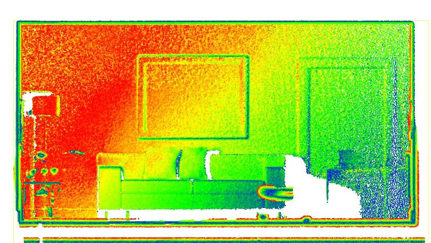
with ξ = [ω ⊤ x⊤ ]⊤ , ω, ∈ R3 and x ∈ R3 .
   Blocks of the combined measurement Jacobian J and resid-
ual r can be populated (while being weighted according to
wrgb ) and solved with a highly parallel tree reduction in
CUDA to produce a 6×6 system of normal equations which is
then solved on the CPU by Cholesky decomposition to yield ξ.
The outcome of this process is an up to date camera pose
estimate Pt = TPt−1 which brings the live camera data Dtl
and Ctl into strong alignment with the current active model
(and hence ready for fusion with the active surfels in M).
                  IV. D EFORMATION G RAPH
   In order to ensure local and global surface consistency in
the map we reflect successful surface loop closures in the set
of surfels M. This is carried out by non-rigidly deforming
all surfels (both active and inactive) according to surface
constraints provided by either of the loop closure methods later
described in Sections V and VI. We adopt a space deformation
approach based on the embedded deformation technique of
Sumner et al. [23].
   A deformation graph is composed of a set of nodes and
edges distributed throughout the model to be deformed. Each
node G n has a timestamp Gtn0 , a position Ggn ∈ R3 and set
of neighbouring nodes N (G n ). The neighbours of each node
                                                                       Fig. 3: Temporal deformation graph connectivity before loop
make up the (directed) edges of the graph. A graph is con-
                                                                       closure. The top half shows a mapping sequence where the
nected up to a neighbour count k such that ∀n, |N (G n )| = k.
                                                                       camera first maps left to right over a desk area and then back
We use k = 4 in all of our experiments. Each node also
                                                                       across the same area. Given the windowed fusion process it
stores an affine transformation in the form of a 3 × 3 matrix
  n                                                                    appears that the map and hence deformation graph is tangled
GR   and a 3 × 1 vector Gtn , initialised by default to the identity
                                                                       up in itself between passes. However, observing the bottom
and (0, 0, 0)⊤ respectively. When deforming a surface, the GR     n
       n                                                               half of the figure where the vertical dimension has been
and Gt parameters of each node are optimised according to
                                                                       artificially stretched by the initialisation times Mt0 and Gt0 of
surface constraints, which we later describe in Section IV-C.
                                                                       each surfel and graph node respectively, it is clear that multiple
   In order to apply a deformation graph to the surface, each
                                                                       passes of the map are disjoint and free to be aligned.
surfel Ms identifies a set of influencing nodes in the graph
I(Ms , G). The deformed position of a surfel is given by:

Mˆ s = φ(Ms ) =
   p
                     X           n  s  n   s    n      n    n
                                w (M ) GR (Mp − Gg ) + Gg + Gt ,       initialise a new deformation graph G each frame with node po-
                        s
                  n∈I(M ,G)                                            sitions set to surfel positions (Ggn = Msp ) and node timestamps
                                                                 (8)   set to surfel initialisation timestamps (Gtn0 = Mst0 ) sampled
while the deformed normal of a surfel is given by:                     from M using systematic sampling such that |G| ≪ |M|.
                                       n −1 ⊤                          Note that this sampling is uniformly distributed over the
           M̂sn =          wn (Ms )GR         Msn ,
                    X
                                                                (9)    population, causing the spatial density of G to mirror that
                            s
                    n∈I(M ,G)                                          of M. The set G is also ordered over n on Gtn0 such that
where wn (Ms ) is a scalar representing the influence node G n         ∀n, Gtn0 ≥ Gtn−1
                                                                                      0
                                                                                         , Gtn−2
                                                                                             0
                                                                                                 , . . . , Gt00 . To compute the connectivity
has on surfel Ms , summing to a total of 1 when n = k:                 of the graph we use this initialisation time ordering of G
                                                                       to connect nodes sequentially up to the neighbour count k,
           wn (Ms ) = (1 − Msp − Ggn         2
                                                 /dmax )2 .    (10)                                                        k
                                                                       defining N (G n ) = {G n±1 , G n±2 , . . . , G n± 2 }. This method is
Here dmax is the Euclidean distance to the k + 1-nearest node          computationally efficient (compared to spatial approaches [23,
of Ms . In the following we describe our method for sampling           1]) but more importantly prevents temporally uncorrelated
the deformation graph G from the set of surfels M along with           areas of the surface from influencing each other (i.e. active
our method for determining graph connectivity.                         and inactive areas), as shown in Figure 3. Note that in the
                                                                       case where n ± k2 is less than zero or greater than |G|
A. Construction                                                        we connect the graph either forwards or backwards from
  Each frame a new deformation graph for the set of surfels            the bound. For example, N (G 0 ) = {G 1 , G 2 , . . . , G k } and
M is constructed, since it is computationally cheap and                N (G |G| ) = {G |G|−1 , G |G|−2 , . . . , G |G|−k }. Next we describe
simpler than incrementally modifying an existing one. We               how to apply the deformation graph to the map of surfels.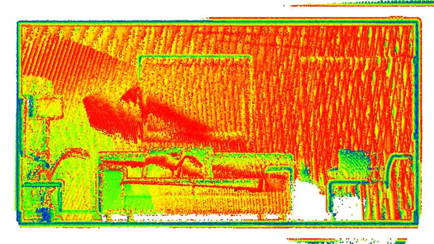
B. Application                                                     position Qps ∈ R3 which should reach the destination upon
   In order to apply the deformation graph after optimisation      deformation. The timestamps of each point are also stored in
(detailed in the next section) to update the map, the set of       Qp as Qpdt and Qpst respectively. We use four cost functions
nodes which influence each surfel Ms must be determined.           over the deformation graph akin to those defined by Sumner
In tune with the method in the previous section a temporal         et al. [23]. The first maximises rigidity in the deformation:
association is chosen, similar to the approach taken by Whelan                              X l ⊤ l             2

et al. [25]. The algorithm which implements I(Ms , G) and                           Erot =       GR GR − I ,                  (11)
                                                                                                                 F
                                                                                                 l
applies the deformation graph G to a given surfel is listed
in Algorithm 1. When each surfel is deformed, the full set of      using the Frobenius-norm. The second is a regularisation term
deformation nodes is searched for the node which is closest in     that ensures a smooth deformation across the graph:
time. The solution to this L1 -norm minimisation is actually a
                                                                                                                                    2
binary search over the set G as it is already ordered. From
                                                                             X     X         l       n   l   l       l   n   n
                                                                    Ereg =                  GR (Gg − Gg ) + Gg + Gt − (Gg + Gt )
                                                                                                                                    2
here, other nodes nearby in time are collected and the k-                    l         l
                                                                                 n∈N (G )
nearest nodes (in the Euclidean distance sense) are selected                                                                       (12)
as I(Ms , G). Finally the weights for each node are computed       The third is a constraint term that minimises the error on the
as in Equation 10 and the transformations from Equations 8         set of position constraints Q, where φ(Qps ) is the result of
and 9 are applied. All other attributes of the updated surfel      applying Equation 8 to Qps :
M̂s are copied from Ms .                                                                                         2
                                                                                                 kφ(Qps ) − Qpd k2
                                                                                             X
                                                                                    Econ =                                   (13)
                                                                                                 p
 Algorithm 1: Deformation Graph Application
                                                                   Note that in order to apply Equation 8 to Qps we must compute
  Input: Ms surfel to be deformed                                  I(Qps , G) and subsequently wn (Qps ). For this we use the same
         G set of deformation nodes                                algorithm as described in Algorithm 1 to deform the position
         α number of nodes to explore                              only, using Qps (inclusive of timestamp Qpst ) in place of Ms .
  Output: M̂s deformed surfel                                      In practice Qpst will always be the timestamp of a surfel within
  do                                                               the active model while Qpdt will be the timestamp of a surfel
     // Find closest node in time                                  within the inactive model. The temporal parameterisation of
      c ← arg min    Mst0 − Gti0                                   the surface we are using allows multiple passes of the same
               i                       1
                                                                   surface to be non-rigidly deformed into alignment allowing
      // Gather set of temporally nearby nodes
                                                                   mapping to continue and new data fusion into revisited areas
      I←∅
                                                                   of the map. Given this, the final cost function “pins” the
      for i ← −α/2 to α/2 do
                                                                   inactive area of the model in place ensuring that we are
          I i+α/2 ← c + i
                                                                   always deforming the active area of the model into the inactive
      sort by euclidean distance(I, G, Msp )                       coordinate system:
      // Take closest k as influencing nodes
                                                                                                                 2
                                                                                                 kφ(Qpd ) − Qpd k2
                                                                                             X
      I(Ms , G) ← I 0→k−1                                                            Epin =                                    (14)
      // Compute weights                                                                         p

      h←0                 k                                        As above we use Algorithm 1 to compute φ(Qpd ), using Qpd
      dmax ← Msp − GgI                                             in place of Ms . The final total cost function is defined as:
                               2
      for n ∈ I(Ms , G) do
                                                                    Edef = wrot Erot + wreg Ereg + wcon Econ + wcon Epin (15)
          wn (Ms ) ← (1 − Msp − Ggn        2
                                               /dmax )2
          h ← h + wn (Ms )                                         With wrot = 1, wreg = 10 and wcon = 100 (in line with
      // Apply transformations                                     related work [23, 1, 25]) we minimise this total cost with
                                                                                 n
       ˆs = P
                           n       s
                          w (M )  n    s        n        n   n   respect to GR   and Gtn over all n using the iterative Gauss-
      M  p         s
              n∈I(M ,G)      h
                                  GR (Mp −      Gg ) + Gg + Gt
       ˆ s  P              n   s
                          w (M ) n −1 ⊤   s
                                                                   Newton algorithm. The Jacobian matrix in this problem is
      Mn = n∈I(Ms ,G)            GR     Mn
                             h                                     sparse and as a result we use sparse Cholesky factorisation
                                                                   to efficiently solve the system on the CPU. From here the
                                                                   deformation graph G is uploaded to the GPU for application
C. Optimisation                                                    to the entire surfel map as described in Section IV-B.
   Given a set of surface correspondences Q (later expanded                          V. L OCAL L OOP C LOSURE
upon in Sections V and VI) the parameters of the deforma-             To ensure local surface consistency throughout the map our
tion graph can be optimised to reflect a surface registration      system closes many small loops with the existing map as those
in the surfel model M. An element Qp ∈ Q is a tuple                areas are revisited. As shown in Figure 2, we fuse into the
Qp = (Qpd ; Qps ; Qpdt ; Qpst ) which contains a pair of points    active area of the model while gradually labeling surfels that
representing a destination position Qpd ∈ R3 and a source          have not been seen in a period of time δt as inactive. The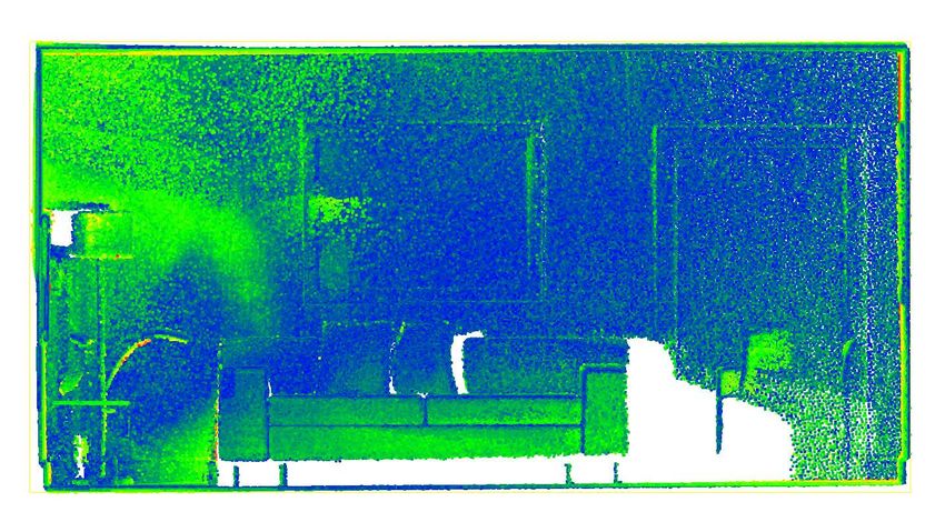
inactive area of the map is not used for live frame tracking of the active model drifting too far from the inactive model for
and fusion until a loop is closed between the active model local alignment to converge, we resort to an appearance-based
and inactive model, at which point the matched inactive area global loop closure method to bootstrap a surface deformation
becomes active again. This has the advantage of continuous which realigns the active model with the underlying inactive
frame-to-model tracking and also model-to-model tracking model for tight global loop closure and surface global consis-
which provides viewpoint-invariant local loop closures. tency. This is described in the following section.
We divide the set of surfels in our map M into two disjoint
sets Θ and Ψ, such that given the current frame timestamp t for VI. G LOBAL L OOP C LOSURE
each surfel in the map Ms ∈ Θ if t − Mst < δt and Ms ∈ Ψ We utilise the randomised fern encoding approach for
if t−Mst ≥ δt , making Θ the active set and Ψ the inactive set. appearance-based place recognition [6]. Ferns encode an RGB-
In each frame if a global loop closure has not been detected D image as a string of codes made up of the values of
(described in the following section), we attempt to compute binary tests on each of the RGB-D channels in a set of fixed
a match between Θ and Ψ. This is done by registering the pixel locations. The approach presented by Glocker et al.
predicted surface renderings of Θ and Ψ from the latest pose includes an automatic method for fern database management
estimate Pt , denoted Dta , Cta and Dti , Cti respectively. This pair that avoids adding redundant views and non-discriminative
of model views is registered together using the same method frames. This technique has been demonstrated to perform very
as described in Section III. The output of this process will be reliably in terms of computational performance and viewpoint
a relative transformation matrix H ∈ SE3 from Θ to Ψ which recognition. Our implementation of randomised fern encoding
brings the two predicted surface renderings into alignment. is identical to that of Glocker et al. with the difference that
In order to check the quality of this registration and decide instead of encoding and matching against raw RGB-D frames,
whether or not to carry out a deformation, we inspect the final we use predicted views of the surface map once they are
condition of the Gauss-Newton optimisation used to align the aligned and fused with the live camera view. Parts of the
two views. The residual cost Etrack from Equation 4 must be predicted views which are devoid of any mapped surface are
sufficiently small, while the number of inlier measurements filled in using the live depth and colour information from the
used must be above a minimum threshold. We also inspect current frame.
the eigenvalues of the covariance of the system (approximated Each frame we maintain a fern encoded frame database E,
by the Hessian as Σ = (J⊤ J)−1 ) by; σi (Σ) < µ for i = using the same process as originally specified by Glocker
{1, . . . , 6}, where σi (Σ) is the i-th eigenvalue of Σ and µ a et al. for fern encoding, frame harvesting and identification
sufficiently conservative threshold. of matching fern encodings [6]. As they suggest, we use a
If a high quality alignment has been achieved, we produce downsampled frame size of 80 × 60. Each element E i ∈ E
a set of surface constraints Q which are fed into the defor- contains a number of attributes; a fern encoding string Efi , a
i
mation graph optimisation described in Section IV to align depth map ED , a colour image ECi , a source camera pose EP
i
the surfels in Θ with those in Ψ. To do this we also require i
and an initialisation time Et . At the end of each frame we
the initialisation timestamps Ψt0 of each surfel splat used to add D̂ta and Cˆta (predicted active model depth and colour after
render Dti . These are rendered as Tti and are necessary to fusion filled in with Dtl and Ctl ) to E if necessary. We also
correctly constrain the deformation between the active model query this database immediate after the initial frame-to-model
and inactive model. We uniformly sample a set of pixel tracking step to determine if there is a global loop closure
coordinates U ⊂ Ω to compute the set Q. For each pixel required. If a matching frame E i is found we perform a number
u ∈ U we populate a constraint: of steps to potentially globally align the surfel map.
Firstly, we attempt to align the matched frame with the
Qp = ((HPt )p(u, Dta ); Pt p(u, Dta ); Tti (u); t). (16)
current model prediction. Similar to the previous section, this
After the deformation has occurred a new up to date camera involves utilising the registration process outlined in Section
pose is resolved as P̂t = HPt . At this point the set of III to bring Dta and Cta into alignment with ED i
and ECi ,
surfels which were part of the alignment are reactivated to including inspection of the final condition of the optimisation.
allow live camera tracking and fusion with the existing active If successful, a relative transformation matrix H ∈ SE3 which
surfels. An up to date prediction of the active model depth brings the current model prediction into alignment with the
must be rendered to reflect the deformation for the depth test matching frame is resolved. From here, as in the previous
for inactive surfels, computed as D̃ta . For each surfel Ms : section, we populate a set of surface constraints Q to provide
as input to the deformation, where each u is a randomly
if π(KP̂−1 s
t t Mp ) ∈ Ω sampled fern pixel location (lifted into full image resolution):
s
Mt = and (KP̂−1 s a −1
t Mp )z . D̃t (π(KP̂t Mp )),
s
s
Mt else. Qp = ((HEP
i
)p(u, Dta ); Pt p(u, Dta ); Eti ; t).
(18)
(17)
The process described in this section brings active areas Note Qpd which incorporates the difference in the estimated
of the model into strong alignment with inactive areas of the point position given by the alignment and the known actual
i
model to achieve tight local surface loop closures. In the event global point position given by EP . From here, the deformation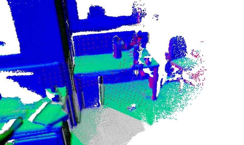
System fr1/desk fr2/xyz fr3/office fr3/nst
DVO SLAM 0.021m 0.018m 0.035m 0.018m
RGB-D SLAM 0.023m 0.008m 0.032m 0.017m
MRSMap 0.043m 0.020m 0.042m 2.018m
Kintinuous 0.037m 0.029m 0.030m 0.031m
Frame-to-model 0.022m 0.014m 0.025m 0.027m
ElasticFusion 0.020m 0.011m 0.017m 0.016m
TABLE I: Comparison of ATE RMSE on the evaluated real
world datasets of Sturm et al. [22].
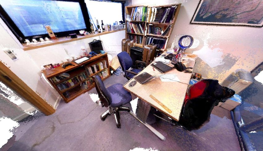
Fig. 4: Orthogonal frontal view heat maps showing reconstruc-
cost from Equations 11-15 is computed and evaluated to tion error on the kt0 dataset. Points more than 0.1m from
determine if the proposed deformation is consistent with the ground truth have been removed for visualisation purposes.
map’s geometry. We are less likely to accept unreliable fern
matching triggered deformations as they operate on a much System kt0 kt1 kt2 kt3
DVO SLAM 0.104m 0.029m 0.191m 0.152m
coarser scale than the local loop closure matches. If Econ RGB-D SLAM 0.026m 0.008m 0.018m 0.433m
is too small the deformation is likely not required and the MRSMap 0.204m 0.228m 0.189m 1.090m
loop closure is rejected (i.e. it should be detected and applied Kintinuous 0.072m 0.005m 0.010m 0.355m
as a local loop closure). Otherwise, the deformation graph Frame-to-model 0.497m 0.009m 0.020m 0.243m
is optimised and the final state of the Gauss-Newton system ElasticFusion 0.009m 0.009m 0.014m 0.106m
is analysed to determine if it should be applied. If after TABLE II: Comparison of ATE RMSE on the evaluated
optimisation Econ is sufficiently small while over all Edef synthetic datasets of Handa et al. [7].
is also small, the loop closure is accepted and the deformation
graph G is applied to the entire set of surfels M. At this
i
point the current pose estimate is also updated to P̂t = HEP . rely on a pose graph optimisation backend. Interestingly our
Unlike in the previous section the set of active and inactive frame-to-model only results are also comparable in perfor-
surfels is not revised at this point. This is for two main reasons; mance, whereas a uniform increase in accuracy is achieved
(i) correct global loop closures bring the active and inactive when active to inactive model deformations are used, proving
regions of map into close enough alignment to trigger a local their efficacy in trajectory estimation. Only on fr3/nst does
loop closure on the next frame and (ii) this allows the map a global loop closure occur. Enabling local loops alone on
to recover from potentially incorrect global loop closures. We this dataset results in an error of 0.022m, while only enabling
also have the option of relying on the fern encoding database global loops results in an error of 0.023m.
for global relocalisation if camera tracking ever fails (however
this was not encountered in any evaluated datasets). B. Surface Estimation
VII. E VALUATION We evaluate the surface reconstruction results of our ap-
proach on the ICL-NUIM dataset of Handa et al. [7]. This
We evaluate the performance of our system both quantita-
benchmark provides ground truth poses for a camera moved
tively and qualitatively in terms of trajectory estimation, sur-
through a synthetic environment as well as a ground truth 3D
face reconstruction accuracy and computational performance.
model which can be used to evaluate surface reconstruction
A. Trajectory Estimation accuracy. We evaluate our approach on all four trajectories in
To evaluate the trajectory estimation performance of our ap- the living room scene (including synthetic noise) providing
proach we test our system on the RGB-D benchmark of Sturm surface reconstruction accuracy results in comparison to the
et al. [22]. This benchmark provides synchronised ground truth same SLAM systems listed in Section VII-A. We also include
poses for an RGB-D sensor moved through a scene, captured trajectory estimation results for each dataset. Tables II and III
with a highly precise motion capture system. In Table I we
compare our system to four other state-of-the-art RGB-D System kt0 kt1 kt2 kt3
based SLAM systems; DVO SLAM [10], RGB-D SLAM [5], DVO SLAM 0.032m 0.061m 0.119m 0.053m
MRSMap [21] and Kintinuous [25]. We also provide bench- RGB-D SLAM 0.044m 0.032m 0.031m 0.167m
mark scores for our system if all deformations are disabled MRSMap 0.061m 0.140m 0.098m 0.248m
Kintinuous 0.011m 0.008m 0.009m 0.150m
and only frame-to-model tracking is used. We use the absolute Frame-to-model 0.098m 0.007m 0.011m 0.107m
trajectory (ATE) root-mean-square error metric (RMSE) in ElasticFusion 0.007m 0.007m 0.008m 0.028m
our comparison, which measures the root-mean-square of the
Euclidean distances between all estimated camera poses and TABLE III: Comparison of surface reconstruction accuracy
the ground truth poses associated by timestamp [22]. These results on the evaluated synthetic datasets of Handa et al. [7].
results show that our trajectory estimation performance is on Quantities shown are the mean distances from each point to
par with or better than existing state-of-the-art systems that the nearest surface in the ground truth 3D model.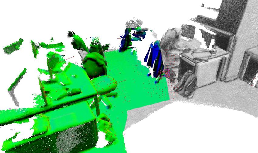
50                                                                      5
                                                                                                    Time
                                                                                       45           Surfels
                                                                                                                                                               4
                                                                                       40

                                                                                                                                                               Millions of Surfels
                                                                                                                                                               3

                                                                        Milliseconds
                                                                                       35

                                                                                       30                                                                      2
                                                                                       25
                                                                                                                                                               1
                                                                                       20

         (i)                   (ii)                     (iii)                          15                                                                      0
                                                                                            0     1,000       2,000    3,000   4,000   5,000   6,000   7,000
                                                                                                                               Frame
Fig. 5: Qualitative datasets; (i) A comprehensive scan of a
copy room; (ii) A loopy large scan of a computer lab; (iii)              Fig. 6: Frame time vs. number of surfels on the Hotel dataset.
A comprehensive scan of a twin bed hotel room (note that
the actual room is not rectilinear). To view small details we
recommend either using the digital zoom function in a PDF
                                                                         understand the capabilities of our approach2 .
reader or viewing of our accompanying videos2 .
                                                                         C. Computational Performance
 Name (Fig.)    Copy (5i)    Lab (5ii)   Hotel (5iii)      Office (1)
                                                                            To analyse the computational performance of the system we
 Frames           5490         6533         7725             5000
                       6            6             6                6     provide a plot of the average frame processing time across the
 Surfels        4.4×10       3.5×10       4.1×10           4.8×10
 Graph nodes       351         282           328              386        Hotel sequence. The test platform was a desktop PC with an
 Fern frames       582         651           325              583        Intel Core i7-4930K CPU at 3.4GHz, 32GB of RAM and an
 Local loops       15           13           11                17        nVidia GeForce GTX 780 Ti GPU with 3GB of memory. As
 Global loops       1            4            1                 0        shown in Figure 6 the execution time of the system increases
        TABLE IV: Statistics on qualitative datasets.                    with the number of surfels in the map, with an overall average
                                                                         of 31ms per frame scaling to a peak average of 45ms implying
                                                                         a worst case processing frequency of 22Hz. This is well
                                                                         within the widely accepted minimum frequencies for fused
summarise our trajectory estimation and surface reconstruction           dense SLAM algorithms [24, 17, 2, 9], and as shown in our
results. Note on kt1 the camera never revisits previously                qualitative results more than adequate for real-time operation.
mapped portions of the map, making the frame-to-model
and ElasticFusion results identical. Additionally, only the kt3                                                       VIII. C ONCLUSION
sequence triggers a global loop closure in our approach. This
yields a local loop only ATE RMSE result of 0.234m and a                    We have presented a novel approach to the problem of
global loop only ATE RMSE result of 0.236m. On surface                   dense visual SLAM that performs time windowed surfel-
reconstruction, local loops only scores 0.099m and global                based dense data fusion in combination with frame-to-model
loops only scores 0.103m. These results show that again our              tracking and non-rigid deformation. Our main contribution in
trajectory estimation performance is on par with or better than          this paper is to show that by incorporating many small local
existing approaches. It is also shown that our surface recon-            model-to-model loop closures in conjunction with larger scale
struction results are superior to all other systems. Figure 4            global loop closures we are able to stay close to the mode of
shows the reconstruction error of all evaluated systems on kt0.          the distribution of the map and produce globally consistent
                                                                         reconstructions in real-time without the use of pose graph
   We also present a number of qualitative results on datasets
                                                                         optimisation or post-processing steps. In our evaluation we
captured in a handheld manner demonstrating system versatil-
                                                                         show that the use of frequent non-rigid map deformations
ity. Statistics for each dataset are listed in Table IV. The Copy
                                                                         improve both the trajectory estimate of the camera and the
dataset contains a comprehensive scan of a photocopying room
                                                                         surface reconstruction quality. We also demonstrate the effec-
with many local loop closures and a global loop closure at one
                                                                         tiveness of our approach in long scale occasionally looping
point to resolve global consistency. This dataset was made
                                                                         camera motions and more loopy comprehensive room scanning
available courtesy of Zhou and Koltun [26]. The Lab dataset
                                                                         trajectories. In future work we wish to address the problem of
contains a very loopy trajectory around a large office envi-
                                                                         map scalability beyond whole rooms and also investigate the
ronment with many global and local loop closures. The Hotel
                                                                         problem of dense globally consistent SLAM as t → ∞.
dataset follows a comprehensive scan of a non-rectilinear hotel
room with many local loop closures and a single global loop
                                                                                                              IX. ACKNOWLEDGEMENTS
closure to resolve final model consistency. Finally the Office
dataset contains a comprehensive scan of a complete office                 Research presented in this paper has been supported by
with many local loop closures avoiding the need for any global           Dyson Technology Ltd.
loop closures for model consistency. We recommend viewing
                                                                                       2
of our accompanying videos to more clearly visualise and                                   https://youtu.be/XySrhZpODYs, https://youtu.be/-dz VauPjEU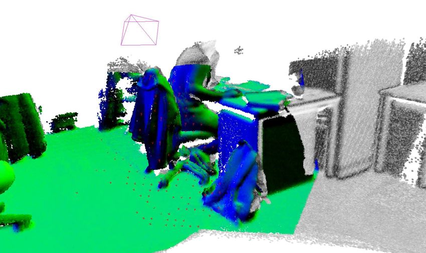
R EFERENCES                                     and voxel-based dense visual SLAM at large scales. In
                                                                        Proceedings of the IEEE/RSJ Conference on Intelligent
 [1] J. Chen, S. Izadi, and A. Fitzgibbon. KinÊtre: animating          Robots and Systems (IROS), 2013.
     the world with the human body. In Proceedings of ACM        [15]   R. A. Newcombe, S. Izadi, O. Hilliges, D. Molyneaux,
     Symposium on User Interface Software and Technolog                 D. Kim, A. J. Davison, P. Kohli, J. Shotton, S. Hodges,
     (UIST), 2012.                                                      and A. Fitzgibbon. KinectFusion: Real-Time Dense
 [2] J. Chen, D. Bautembach, and S. Izadi. Scalable real-               Surface Mapping and Tracking. In Proceedings of
     time volumetric surface reconstruction. In Proceedings             the International Symposium on Mixed and Augmented
     of SIGGRAPH, 2013.                                                 Reality (ISMAR), 2011.
 [3] A. J. Davison. Real-Time Simultaneous Localisation and      [16]   R. A. Newcombe, S. Lovegrove, and A. J. Davison.
     Mapping with a Single Camera. In Proceedings of the                DTAM: Dense Tracking and Mapping in Real-Time. In
     International Conference on Computer Vision (ICCV),                Proceedings of the International Conference on Com-
     2003.                                                              puter Vision (ICCV), 2011.
 [4] A. J. Davison, N. D. Molton, I. Reid, and O. Stasse.        [17]   R. F. Salas-Moreno, B. Glocker, P. H. J. Kelly, and
     MonoSLAM: Real-Time Single Camera SLAM. IEEE                       A. J. Davison. Dense Planar SLAM. In Proceedings of
     Transactions on Pattern Analysis and Machine Intelli-              the International Symposium on Mixed and Augmented
     gence (PAMI), 29(6):1052–1067, 2007.                               Reality (ISMAR), 2014.
 [5] F. Endres, J. Hess, N. Engelhard, J. Sturm, D. Cremers,     [18]   F. Steinbrucker, C. Kerl, J. Sturm, and D. Cremers.
     and W. Burgard. An evaluation of the RGB-D SLAM                    Large-scale multi-resolution surface reconstruction from
     system. In Proceedings of the IEEE International Con-              RGB-D sequences. In Proceedings of the International
     ference on Robotics and Automation (ICRA), 2012.                   Conference on Computer Vision (ICCV), 2013.
 [6] B. Glocker, J. Shotton, A. Criminisi, and S. Izadi. Real-   [19]   F. Steinbrucker, J. Sturm, and D. Cremers. Volumetric
     Time RGB-D Camera Relocalization via Randomized                    3d mapping in real-time on a CPU. In Proceedings
     Ferns for Keyframe Encoding. IEEE Transactions on                  of the IEEE International Conference on Robotics and
     Visualization and Computer Graphics, 21(5):571–583,                Automation (ICRA), 2014.
     2015.                                                       [20]   H. Strasdat, A. J. Davison, J. M. M. Montiel, and
 [7] A. Handa, T. Whelan, J. B. McDonald, and A. J. Davi-               K. Konolige. Double Window Optimisation for Constant
     son. A Benchmark for RGB-D Visual Odometry, 3D                     Time Visual SLAM. In Proceedings of the International
     Reconstruction and SLAM. In Proceedings of the IEEE                Conference on Computer Vision (ICCV), 2011.
     International Conference on Robotics and Automation         [21]   J. Stückler and S. Behnke. Multi-resolution surfel maps
     (ICRA), 2014. URL http://www.doc.ic.ac.uk/∼ahanda/                 for efficient dense 3d modeling and tracking. Journal of
     VaFRIC/iclnuim.html.                                               Visual Communication and Image Representation, 25(1):
 [8] P. Henry, D. Fox, A. Bhowmik, and R. Mongia. Patch                 137–147, 2014.
     Volumes: Segmentation-based Consistent Mapping with         [22]   J. Sturm, N. Engelhard, F. Endres, W. Burgard, and
     RGB-D Cameras. In Proc. of Joint 3DIM/3DPVT Con-                   D. Cremers. A benchmark for RGB-D SLAM evalu-
     ference (3DV), 2013.                                               ation. In Proceedings of the IEEE/RSJ Conference on
 [9] M. Keller, D. Lefloch, M. Lambers, S. Izadi, T. Weyrich,           Intelligent Robots and Systems (IROS), 2012.
     and A. Kolb. Real-time 3D Reconstruction in Dynamic         [23]   R. W. Sumner, J. Schmid, and M. Pauly. Embedded
     Scenes using Point-based Fusion. In Proc. of Joint                 deformation for shape manipulation. In Proceedings of
     3DIM/3DPVT Conference (3DV), 2013.                                 SIGGRAPH, 2007.
[10] C. Kerl, J. Sturm, and D. Cremers. Dense visual SLAM        [24]   T. Whelan, J. B. McDonald, M. Kaess, M. Fallon,
     for RGB-D cameras. In Proceedings of the IEEE/RSJ                  H. Johannsson, and J. J. Leonard. Kintinuous: Spatially
     Conference on Intelligent Robots and Systems (IROS),               Extended KinectFusion. In Workshop on RGB-D: Ad-
     2013.                                                              vanced Reasoning with Depth Cameras, in conjunction
[11] G. Klein and D. W. Murray. Parallel Tracking and                   with Robotics: Science and Systems, 2012.
     Mapping for Small AR Workspaces. In Proceedings of          [25]   T. Whelan, M. Kaess, H. Johannsson, M. F. Fallon, J. J.
     the International Symposium on Mixed and Augmented                 Leonard, and J. B. McDonald. Real-time large scale
     Reality (ISMAR), 2007.                                             dense RGB-D SLAM with volumetric fusion. Interna-
[12] K. Konolige and M. Agrawal. FrameSLAM: From                        tional Journal of Robotics Research (IJRR), 34(4-5):598–
     Bundle Adjustment to Real-Time Visual Mapping. IEEE                626, 2015.
     Transactions on Robotics (T-RO), 24:1066–1077, 2008.        [26]   Q. Zhou and V. Koltun. Dense scene reconstruction with
[13] J. B. McDonald, M. Kaess, C. Cadena, J. Neira, and J. J.           points of interest. In Proceedings of SIGGRAPH, 2013.
     Leonard. Real-time 6-DOF multi-session visual SLAM          [27]   Q. Zhou, S. Miller, and V. Koltun. Elastic Fragments
     over large scale environments. Robotics and Autonomous             for Dense Scene Reconstruction. In Proceedings of the
     Systems, 61(10):1144–1158, 2013.                                   International Conference on Computer Vision (ICCV),
[14] M. Meilland and A. I. Comport. On unifying key-frame               2013.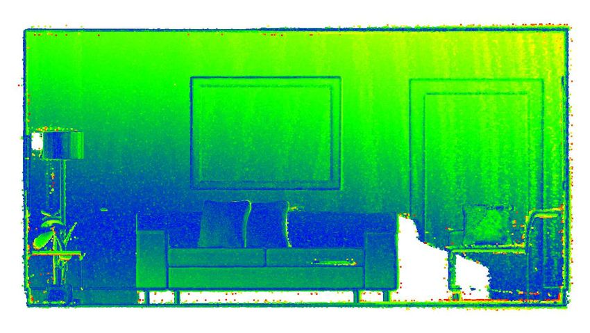
You can also read