Beyond accuracy: Measures for assessing machine learning models, pitfalls and guidelines - bioRxiv
←
→
Page content transcription
If your browser does not render page correctly, please read the page content below
bioRxiv preprint first posted online Aug. 22, 2019; doi: http://dx.doi.org/10.1101/743138. The copyright holder for this preprint
 (which was not peer-reviewed) is the author/funder, who has granted bioRxiv a license to display the preprint in perpetuity.
                                It is made available under a CC-BY-NC 4.0 International license.

     Beyond accuracy: Measures for assessing machine learning models, pitfalls and
     guidelines
     Richard Dingaa,b, Brenda W.J.H. Penninxa, Dick J. Veltmana, Lianne Schmaalc,d*, Andre F.
     Marquandb*
     a
       Department of Psychiatry, Amsterdam UMC, Amsterdam, the Netherlands
     b
       Donders Institute for Brain, Cognition and Behaviour, Radboud University, Nijmegen, the
     Netherlands
     c
       Orygen, The National Centre of Excellence in Youth Mental Health, Parkville, Australia
     d
       Centre for Youth Mental Health, The University of Melbourne, Melbourne, Australia
     *
       These authors contributed equally

     Abstract
     Pattern recognition predictive models have become an important tool for analysis of neuroimaging
     data and answering important questions from clinical and cognitive neuroscience. Regardless of the
     application, the most commonly used method to quantify model performance is to calculate
     prediction accuracy, i.e. the proportion of correctly classified samples. While simple and intuitive,
     other performance measures are often more appropriate with respect to many common goals of
     neuroimaging pattern recognition studies. In this paper, we will review alternative performance
     measures and focus on their interpretation and practical aspects of model evaluation. Specifically,
     we will focus on 4 families of performance measures: 1) categorical performance measures such as
     accuracy, 2) rank based performance measures such as the area under the curve, 3) probabilistic
     performance measures based on quadratic error such as Brier score, and 4) probabilistic
     performance measures based on information criteria such as logarithmic score. We will examine
     their statistical properties in various settings using simulated data and real neuroimaging data
     derived from public datasets. Results showed that accuracy had the worst performance with respect
     to statistical power, detecting model improvement, selecting informative features and reliability of
     results. Therefore in most cases, it should not be used to make statistical inference about model
     performance. Accuracy should also be avoided for evaluating utility of clinical models, because it
     does not take into account clinically relevant information, such as relative cost of false-positive and
     false-negative misclassification or calibration of probabilistic predictions. We recommend
     alternative evaluation criteria with respect to the goals of a specific machine learning model.

     Introduction

     Machine learning predictive models have become an integral method for many areas of clinical and
     cognitive neuroscience, including classification of patients with brain disorders from healthy
     controls, treatment response prediction or, in a cognitive neuroscience setting, identifying brain
     areas containing information about experimental conditions. They allow making potentially
     clinically important predictions and testing hypotheses about brain function that would not be
     possible using traditional mass univariate methods (i.e., effects distributed across multiple
     variables). Regardless of the application, it is important to evaluate the quality of predictions on
     new, previously unseen data.

     A common method to estimate the quality of model predictions is to use cross-validation and
     calculate the average prediction performance across test samples (Varoquaux et al., 2017) or
     balanced variants that account for different class frequencies (Brodersen et al., 2010) Selection of
     appropriate performance measures is a widely studied topic in other areas of science, such as
     weather forecasting (Mason, 2008), medicine (Steyerberg et al., 2010) or finance ((Hamerle et al.,
     2003). However, in the neuroimaging field, this has received surprisingly little attention. For
     example, many introductory review and tutorial articles focused on machine learning in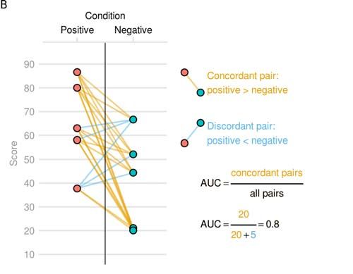
bioRxiv preprint first posted online Aug. 22, 2019; doi: http://dx.doi.org/10.1101/743138. The copyright holder for this preprint
 (which was not peer-reviewed) is the author/funder, who has granted bioRxiv a license to display the preprint in perpetuity.
                                It is made available under a CC-BY-NC 4.0 International license.

     neuroimaging (Haynes and Rees, 2006; Pereira et al., 2009; Varoquaux et al., 2017) do not discuss
     performance measures other than accuracy (i.e., simple proportion of correctly classified samples).
     Accuracy is also the most frequently reported performance measure in neuroimaging studies
     employing machine learning, even though in many cases alternative performance measures may be
     more appropriate for the specific problem at hand. However, no performance measure is perfect and
     suitable for all situations and different performance measures capture different aspects of model
     predictions. Thus, a thoughtful choice needs to be made in order to evaluate the model predictions
     based on what is important in each specific situation. Different performance measures also have
     different statistical properties which need to be taken into account. For example, how reliable or
     reproducible are the results, or what is the power of detecting a statistically significant effect?

     In this paper, we provide a didactic overview of various performance measures focusing on their
     interpretation and practical aspects of their usage. We divide the measures into four families based
     on what aspects of a model prediction they evaluate; (1) measures evaluating categorical
     predictions, (2) ranks of predictions, (3) probabilistic predictions with respect to a squared error,
     and (4) probabilistic predictions with respect to information criteria. This includes accuracy, the
     area under the receiver operating characteristic curve, the Brier score, and the logarithmic score
     respectively, as most prominent members of each family. Next, we perform an extensive empirical
     evaluation of statistical properties of these measures, focusing on power to detect a statistically
     significant effect, power to detect a model improvement, evaluation of stability of the feature
     selection process, and evaluation of the reliability of results. We show that accuracy performs the
     worst with respect to all examined statistical properties. Last, we discuss appropriate evaluation
     criteria with respect to various goals of the specific machine learning model.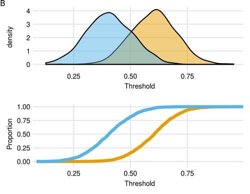
bioRxiv preprint first posted online Aug. 22, 2019; doi: http://dx.doi.org/10.1101/743138. The copyright holder for this preprint
(which was not peer-reviewed) is the author/funder, who has granted bioRxiv a license to display the preprint in perpetuity.
It is made available under a CC-BY-NC 4.0 International license.
Tutorial on performance measures
This section is a didactic overview of 4 main types of performance measures.
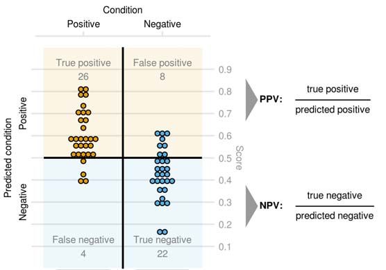
Figure 1: Definition of categorical predictions and their relationship to a confusion matrix. Note
that the predicted score (e.g. predicted probability from a logistic regression, here depicted by the
position of the predictions on the y-axis) needs to be dichotomized into categorical predictions, thus
the magnitude of a miss-classification is not taken into account. Balanced accuracy equals
accuracy when the class frequencies are equal, otherwise misclassification of the minority class is
weighted higher, therefore, the chance level stays at 0.5. PPV: positive predictive value. NPV:
Negative predictive value.
Categorical measures
The most commonly used performance measures are based on an evaluation of categorical
predictions. These can be derived from a confusion matrix where predicted labels are displayed in
rows and observed labels are displayed in columns (Figure 1). The most commonly used measure is
accuracy, which is a simple proportion of all samples classified correctly. This can be misleading in
imbalanced classes, since for example if the disease prevalence is 1% it is trivial to obtain an
accuracy of 99% just by always reporting no disease. For this reason, balanced accuracy is often
used instead (Brodersen et al., 2010). Balanced accuracy is simply the arithmetic mean of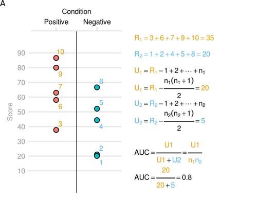
bioRxiv preprint first posted online Aug. 22, 2019; doi: http://dx.doi.org/10.1101/743138. The copyright holder for this preprint
 (which was not peer-reviewed) is the author/funder, who has granted bioRxiv a license to display the preprint in perpetuity.
                                It is made available under a CC-BY-NC 4.0 International license.

     sensitivity and specificity, thus it is equal to accuracy when the class frequencies are the same
     (Figure 1), otherwise, because sensitivity and specificity are contributing equally, it weighs false
     positive and false negative miss classifications according to class frequencies.

     Sensitivity (true positive rate, recall) is the proportion of positive samples classified as positive, or
     in other words, it is the probability that a sample from a positive class will be classified as positive.
     Specificity (true negative rate) is the counterpart to sensitivity measuring the proportion of negative
     samples correctly classified as negative. Sensitivity and specificity do not take class frequencies
     (and class imbalances) or disease prevalence into account and they do not capture what is important
     in many practical applications. For example, in a clinical setting, we don’t know if the patient has a
     disease or not (otherwise, there would be no need for testing).Instead, what is known are the results
     of the test (positive or negative) and we would like to know, given the result of the test, what is the
     probability that the patient will have a disease or not. This is measured by positive predictive value
     (PPV) and negative predictive value (NPV) for positive and negative test results, respectively. It is
     easy to misinterpret sensitivity as PPV, the difference is subtle but crucial. To illustrate, say we
     have the following confusion matrix:

                                      Condition
                                      Positive Negative
      Predicted        Positive       10            90
      Condition        Negative 0                   900

     This gives us 100% sensitivity (10/10, 91% specificity (900/990), 91% accuracy ((10+900)/1000)
     and 96% balanced accuracy ((10/10 + 900/990)/2). According to these measures, the model
     performs well. However, in this example the disease prevalence is 1% (10/1000), so only 10% of
     patients with a positive test result are truly positive, the remaining 90% are misclassified (i.e., cell
     with positive predicted condition but negative actual condition in confusion matrix). Therefore, the
     test may actually be useless in practice. Another measure used in cases with imbalanced classes is
     the F1 score, which is the harmonic mean of PPV and sensitivity (so if one of the elements is close
     to 0, the whole score will be close to 0) (Figure 1). Since the harmonic and not the arithmetic mean
     is used, both sensitivity and PPV need to be high in order for the score to be high. Thus, this score
     emphasizes the balance between sensitivity and PPV and it assumes that both are equally important.

     All categorical measures suffer from two main problems: first, they depend on an arbitrarily
     selected classification threshold. Each data point counts either as a correct or incorrect
     classification, without taking the magnitude of the error into account. If the decision threshold is set
     to 50%, then if a model predicts that a disease probability in a healthy subject is 49% percent and
     thus classifies this subject as healthy, this is indistinguishable from a disease probability of 1% in
     another healthy subject (also classified as healthy). Imagine two models, one predicts that a healthy
     subjects has a disease with a probability of 99% and other with a probability of 51%. The latter
     model is obviously better since the error is smaller, but if these predictions are thresholded at
     traditional 50% percent, the accuracy will not be able to detect the improvement. Due to this
     insensitivity, compared to measures that do not require dichotomization of predictions, using
     accuracy necessarily leads to a significant loss of statistical power. Second, false positive and false
     negative misclassification are weighted as being equally bad or according to class frequencies
     (balanced accuracy), which is often inappropriate. Rather, misclassification costs are asymmetric
     and depend on consequences of such misclassification. For example, in a clinical context,
     misclassifying a healthy subject as diseased is worse when this misclassification will lead to an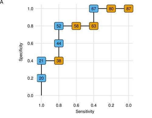
bioRxiv preprint first posted online Aug. 22, 2019; doi: http://dx.doi.org/10.1101/743138. The copyright holder for this preprint
 (which was not peer-reviewed) is the author/funder, who has granted bioRxiv a license to display the preprint in perpetuity.
                                It is made available under a CC-BY-NC 4.0 International license.

     unnecessary open brain surgery, than when it will lead to a prescription of medications with no side
     effects.

     One way to combat unequal misclassification cost is to select the decision threshold according to
     cost-benefit analysis, such that the action is made when the expected benefit of the action outweighs
     the expected harm. This is then evaluated by cost-weighted accuracy, where true positives and false
     positives are weighted according to their relative cost. Although this allows to evaluate categorical
     predictions according to their utility and not arbitrarily, the dichotomization still creates problems
     for many practical applications. For example, in a clinical setting, the categorized predictions hide
     potentially useful clinical information from decision-makers (be it clinician, patient, an insurance
     company, etc.). If a prediction is only the presence versus the absence of a disease, a decision maker
     cannot take into account if a probability of the disease is 1%, 15% or 40%. This effectively moves
     the decision from stakeholders to a data analyst assuming that the chosen decision threshold is
     appropriate and constant for every situation and every patient, thus not allowing to take clinicians’
     opinions or patients’ preferences into account.

     Rank based measures
     Another important family of performance measures are those based on ranks of predictions. Here,
     predictions are not categorical, but all predictions are ranked from lowest to highest with respect to
     the probability of an outcome.

     The most common measure from this family is the area under the receiver operating characteristic
     curve (AUC). It measures a separation between two distributions, with a maximum score of 1
     meaning perfect separation or no overlap between distributions and 0.5 being chance level when the
     distributions cannot be separated. In the case of model evaluation, the two distributions are
     distributions of predicted values (e.g. probability of a disease) for each target group. AUC is
     identical or closely related to multiple more or less known concepts, some of which we will review
     below.

     The most common way of interpreting the AUC is through the receiver operating characteristic
     curve (ROC) (Figure 2A). This is a plot showing how a proportion of false positive and false
     negative misclassifications (i.e. sensitivity and specificity) changes as a function of the decision
     threshold. AUC is then the area under this curve. The curve itself is useful because it visualizes
     sensitivity and specificity across all thresholds not only for one threshold as in the case with the
     confusion matrix. Thus it allows choosing a decision threshold with an appropriate balance between
     sensitivity and specificity. We can see that if a model has no predictive power, then regardless of
     the threshold, the proportion of false positives and false negatives will always sum to 1, therefore
     the ROC curve will be a straight line across the diagonal and thus the area under this curve will be
     0.5.

     AUC can also be seen as quantifying to which extent two distributions overlap. We can rearrange
     the ROC plot, in such a way that the threshold value is on the x-axis and two curves are shown, one
     for the false-negative rate (1-sensitivity) and one for the true negative rate, both on the y-axis. The
     area between the diagonal and the ROC curve in the ROC plot (Figure 2A) is now the area between
     these two curves. These two curves are cumulative distributions of subjects from each class. The
     area between these curves represents the non-overlapping areas of two distributions (Figure 2B).

     AUC is identical to C-index or a concordance probability in the case of a binary outcome (Hanley
     and McNeil, 1982). This is the probability that a randomly chosen data point forms a positive class
     is ranked higher than a randomly chosen example forms the negative class. E.g. if we have two
     patients, one with disease and one without, AUC is the probability that the model will correctly rank
     patients with a disease to have a higher risk of the disease than patients without the disease. This
bioRxiv preprint first posted online Aug. 22, 2019; doi: http://dx.doi.org/10.1101/743138. The copyright holder for this preprint
(which was not peer-reviewed) is the author/funder, who has granted bioRxiv a license to display the preprint in perpetuity.
It is made available under a CC-BY-NC 4.0 International license.
can also be interpreted as a proportion of all pairs of subjects in the dataset, where a subject with the
disease is ranked higher than a subject without the disease (Figure 3B).
AUC is also a rescaling of several rank-based correlation measures, including Sommers dxy
(Newson, 2002) . It is also a normalized Mann-Whitney U statistic (Mason and Graham, 2002),
which is used in the Mann-Whitney U test or Wilcoxon rank-sum test, a popular nonparametric
alternative for a t-test. The latter connection is especially important because it means that by testing
the statistical significance of a difference between two groups using the Mann-Whitney U test, one
is also testing the statistical significance of AUC and vice versa (Figure 3A).
Figure 2. A: ROC curve for the same data as in Figure 3. The points on the curve represent
threshold values that divide continuous prediction into two classes (represented as orange and blue
colors). B: AUC as an overlap between two distributions. Two distributions (top) are transformed
into cumulative distribution (bottom). The non-overlapping area of these two distributions is the
area between two cumulative distribution curves, which equals to the area between the diagonal to
the ROC curve or AUC – 0.5.bioRxiv preprint first posted online Aug. 22, 2019; doi: http://dx.doi.org/10.1101/743138. The copyright holder for this preprint
(which was not peer-reviewed) is the author/funder, who has granted bioRxiv a license to display the preprint in perpetuity.
It is made available under a CC-BY-NC 4.0 International license.
Figure 3. Interpretation and construction of AUC from the figure 2A as an A) sum of ranks, i.e.
Mann-Whitney U statistics. Predictions are ranked from lowest to highest, and the sum of ranks R1
for the positive class is computed (or R2 for negative class). From the sum of ranks, Mann-Whitney
U statistic is computed by subtracting the sum of ranks of one group from the sum of ranks of all
predictions. AUC is the normalized version of the Mann-Whitney U, by dividing U statistics by the
maximum possible value of the U statistics and B) concordance measure. AUC can be interpreted
as a proportion of pairs of subjects where a subject from the positive class is ranked higher than a
subject from the negative class, or where a randomly selected subject from the positive class is
ranked higher than a randomly selected subject from the negative class.
Quadratic error-based measures
Performance measures based on the quadratic error (together with information-based measures)
quantify the performance of probabilistic predictions directly, without any intermediate
transformation of predictions to categorical predictions or ranks. This makes them the most
sensitive measures to capture signal in the data or model improvement, although it requires that the
model predictions are in the form of probabilities.
Brier score (Brier, 1950)is the most prominent example from this category. It is a mean squared
error between predicted values and observed values, where predictions are coded as 0 and 1, for the
case of the binary classifier. The Brier score can be straightforwardly generalised to multi-class
classification using ‘one-hot’ dummy coding.bioRxiv preprint first posted online Aug. 22, 2019; doi: http://dx.doi.org/10.1101/743138. The copyright holder for this preprint
(which was not peer-reviewed) is the author/funder, who has granted bioRxiv a license to display the preprint in perpetuity.
It is made available under a CC-BY-NC 4.0 International license.
Brier =
ଵ
∑ୀଵ ଶ
For example, if a model predicts that a patient with a disease has a disease with a probability of 0.8,
the squared error will be (1-0.8)^2=0.04 and the Brier score is the average of error of all predictions
across all subjects. Brier score has values between 0 and 1 (smaller the better), with 0.25 for a
chance level predictions in a case where there is an equal number of subjects in both groups
(because 0.5^2=0.25). Compared to AUC, it takes into account specifically predicted probabilities
of an outcome, not only their ranks. The score is improved when the predictions are well calibrated,
so when the predicted probabilities correspond to observed frequencies of misclassification (e.g. in
subjects with the predicted probability of a disease of 0.8 , 80% of these subjects will have the
disease).
One of the difficulties with employing the Brier score in practice is that – unlike accuracy and AUC
– it lacks a simple intuitive interpretation. In order to make it more intuitive, it can be rescaled to
form a pseudo R2 measure analogous to variance explained used in evaluate regression models.
The Scaled Brier score is defined as
Brierscaled = 1
where the Briermax is the maximum score that can be obtained with a non-informative model
Briermax=
ଵ
∑ୀଵ 1 ଵ ∑ୀଵ
Thus a non-informative model will have a score of 0 and a perfect model score of 1, regardless of
class frequencies.
One intuitively interpretable measure is a discrimination slope, also known as Tjur’s pseudo R2
(Tjur, 2009).
Tjur’s pseudo R2 =
ଵ
∑ୀଵ ଵ ∑ୀଵ
This is simply the difference between the mean of predicted probabilities of two classes, which can
also be easily visualized (Figure 4).
Figure 4: Tjur’s pseudo R2. Interpretation of Tjur’s pseudo R2 is the difference between mean
predicted probability of the positive group and the negative group.
Information criteriabioRxiv preprint first posted online Aug. 22, 2019; doi: http://dx.doi.org/10.1101/743138. The copyright holder for this preprint
(which was not peer-reviewed) is the author/funder, who has granted bioRxiv a license to display the preprint in perpetuity.
It is made available under a CC-BY-NC 4.0 International license.
Information theory provides a natural framework to evaluate the quality of model predictions
according to how much information about the outcome is contained in the probabilistic predictions.
The most important information-theoretical measure is the logarithmic score, defined as
Logarithmic score = ௧௧
where p_target is the predicted probability of the observed target. If the target is coded as 0 and 1,
and the score is averaged across all predictions, this becomes
Logarithmic score =
ଵ
∑ୀଵ 1 1
For example, a model predicts that a patient with a disease has a disease with a probability of 0.8,
the logarithmic score will be ln(0.8) = -0.22. It has many interpretations and strong connections to
other important mathematical concepts. It is a log-likelihood of observed outcomes given model
predictions, it also equals to Kullback–Leibler or relative entropy between observed target values
and predicted probabilities. It quantifies an average information loss (in bits) about the target given
that we have only imperfect, probabilistic predictions. It also quantifies how surprising the observed
targets are given the probabilistic predictions. In a certain sense, the logarithmic score is an optimal
score. It has been shown that in betting or investing, the expected long term gains are directly
proportional to the amount of information the gambler has about the outcome. For example, if two
gamblers are betting against each other repeatedly on an outcome of football games, the gambler
whose predictions are better according to the logarithmic score, will on average multiply her wealth,
even if her predictions might be worse according to Brier score or AUC (Kelly, 1956; Roulston and
Smith, 2000).
In practice, the logarithmic score and Brier score usually produce similar results and the difference
is evident only with severe misclassification. The logarithmic score can grow to infinity when the
predicted probability of an outcome is close to zero.
This might be considered undesirable since a single extreme wrong prediction can severely affect
the summary score of an otherwise well-performing model. On the other hand, it can be argued that
this is a desirable property of a score and predictions close to 0 and 1 should be discouraged.
Intuitively, the logarithmic score measures surprise, if an event that is supposed to be absolutely
impossible (p=0) happens, we rightly ought to be infinitely surprised. Similarly, if we know that an
event is absolutely certain (p=1), then the right approach (mathematically) would be to bet all our
money on this event, thus it is desirable that the wrong prediction is maximally penalized.
Similarly to the Brier score, the logarithmic score can be scaled to make it more intuitively
interpretable. One popular way is to use Nagelkerke pseudo R2 (Nagelkerke, 1991) which is defined
as
൰⁄
R2Nagelkerke =
ଵି൬
ଵିሺ ሻ⁄
Where L(P) is a logarithmic score of model and L(Pnull) is a logarithmic score of chance level
predictions (i.e. predicting only class frequencies).
Empirical evaluation
Here we perform several empirical evaluations of statistical properties of the selected performance
measures, one from each family described above, namely, accuracy, AUC, Brier score and
logarithmic score. We examine: (i) the statistical power of detecting a statistically significant result,bioRxiv preprint first posted online Aug. 22, 2019; doi: http://dx.doi.org/10.1101/743138. The copyright holder for this preprint
(which was not peer-reviewed) is the author/funder, who has granted bioRxiv a license to display the preprint in perpetuity.
It is made available under a CC-BY-NC 4.0 International license.
(ii) the power to detect a statistically significant improvement in model performance, (iii) the
feature selection stability, and (iv) the reliability of cross-validation results. We employ real and
simulated datasets.
Statistical power of detecting a statistically significant result
Statistical tests: In this section, we evaluate how often a given method is likely to detect a
statistically significant effect (i.e., a classifier that exceeds chance levels at a given significance
level, nominally p < 0.05). In this case, the focus is on statistical significance, but not on the
absolute level of performance. We used the same datasets using the different performance measures
described above. We tested the power of a model to make a statistically significant prediction on an
independent test set. Statistical significance of the accuracy measure was obtained using a binomial
test. To obtain statistical significance of AUC, we performed Mann-Whitney U test. Since AUC is
equivalent to Wilcoxon-Mann-Whitney U statistics, performing Mann-Whitney-U test on model
predictions equals to performing a statistical significance test of AUC. P-values for Brier score and
log score were obtained using a permutation test, where the real labels were shuffled for a
maximum of 10,000 times and the specific scores were computed for each shuffle, thus obtaining an
empirical null distribution of scores where the specific p-value corresponds to a percentile of the
observed test statistic in this distribution. For permutation tests, we employed early stopping criteria
according to (Gandy, 2009), that stopped the permutation when the chance of making wrong
decision to reject the null hypothesis was lower than 0.001. Performing the permutation test for
accuracy and AUC is not necessary, because their distributions are known and can be computed
exactly. These tests are only valid because we are testing the statistical significance in an
independent test set. However, they would produce overly optimistic results in a cross-validation
setting. This is because data points between folds are no longer completely independent and a
permutation test where a model is refitted in each permutation should be used instead (Noirhomme
et al., 2014; Varoquaux et al., 2017).
Experiments:
First, we examined statistical power on simulated distributions of model predictions, without any
machine learning modeling. Similar to the first experiment, we repeatedly sampled from two one-
dimensional Gaussian distributions 1 SD apart representing the distribution of model predictions of
two classes. These predictions were transformed into 0-1 range using a logistic function and into
categorical predictions by thresholding at 0.5 threshold. We performed 1000 simulations for sample
sizes 20, 80, 140, 200, and recorded proportion of times each statistical test obtained a statistically
significant result (p < 0.05).
Second, we examined statistical power of a support vector machine (SVM) to discriminate between
two groups in the simulated dataset. The simulated dataset consisted of 6 independent variables, 3
signal variables and 3 noise variables. Signal variables were each randomly sampled from a
Gaussian distribution with SD=1 and mean=0 for group 0 and mean=0.3 for group 1. Three noise
variables were each randomly sampled from a Gaussian distribution with mean=0 and SD=1. We
repeatedly sampled training and test set from this dataset of size 40, 80, 120, 140, and fit a support
vector machine classifier in the training set and evaluated the statistical significance of the
predictions in the test set. We used C-SVM implementation of an SVM with a linear kernel from a
package kernlab (Karatzoglou et al., 2004), with a C parameter fixed at 1. SVM predictions were
transformed into probabilities using Platt scaling (Platt, 1999), as implemented in kernlab.
Third, we examined statistical power on real neuroimaging datasets, including OASIS cross-
sectional (Marcus et al., 2010) and ABIDE datasets (Craddock et al., 2009). We used already
preprocessed OASIS VBM data as provided by the OASIS project using nilearn dataset fetchingbioRxiv preprint first posted online Aug. 22, 2019; doi: http://dx.doi.org/10.1101/743138. The copyright holder for this preprint
(which was not peer-reviewed) is the author/funder, who has granted bioRxiv a license to display the preprint in perpetuity.
It is made available under a CC-BY-NC 4.0 International license.
functionality (Abraham et al., 2014) The preprocessing consisted of brain extraction, segmentation
of white matter and gray matter, and normalization to standard space using DARTEL. Details of the
preprocessing can be found elsewhere (Marcus et al., 2010). Here we used gray matter and white
matter data separately in order to predict biological sex and diagnostic status (presence or absence
of dementia). To reduce the computational load, we reduced the dimensionality of the WM and GM
datasets to 100 principal components each. Furthermore, we used already preprocessed ABIDE
dataset as provided by the preprocessed-connectome-project (Craddock et al., 2009)to predict
biological sex. These consisted of ROI average cortical thickness data obtained using ANTs
pipeline (Das et al., 2009), defined using sulcus landmarks according to the Desikan-Killiany-
Tourville (DKT) protocol (Klein and Tourville, 2012).
Additionally, we included common non-imaging machine learning benchmark datasets obtained
from using mlbench and kernlab libraries originaly from UCI machine learning repository (Dua and
Graff, 2017). These included Pima Indians diabetes, sonar, musk, and spam.
Finally, in order to compare statistical power to detect statistically significant above chance
prediction according to specific performance measures, it is important to show that the higher
power is due to higher sensitivity of the performance measure and not because the used statistical
test is overly optimistic. To do this, we repeated all experiments including simulated and real
datasets, but with permuting true labels before each simulation to destroy any relationship between
the data and target outcome.
Results: In all simulated and real datasets, when the null hypothesis was true (i.e. performing
experiments on data with shuffled labels), statistical significance p < 0.05 was obtained
approximately 5% of times for significance tests of AUC, Brier score and logarithmic score, as
expected (supplementary figure 1). The binomial test was often overly conservative, i.e., p < 0.05
was obtained less than 5% of times. This is a known behavior of binomial test in small samples
caused by a limited number of values in the null distribution (Fig 4 shows the example of n=20
sample). This conservativeness is worse in small samples and it disappears when the sample size is
sufficiently large (i.e. N=5000). This behavior is not limited to a binomial test, it also happens if the
p-value of accuracy is calculated using permutation test, which is just a random approximation of
the exact binomial test, and the low resolution of the null distribution of accuracy results is present
even when this distribution is obtained using permutations.
For all experiments and all sample sizes, tests using accuracy had the lowest power. Brier score,
logarithmic score, and AUC performed approximately the same. At the sample size where AUC,
Brier score, the logarithmic score obtained the common goal of 80% power, accuracy obtained only
60% power in all datasets (see figure 5). Results for all datasets separately are in supplementary
figure 2
Fig 5: Null distribution of correct predictions for n=20 illustrating why significance test for
categorical predictions is conservative in small samples at specific significance levels. Since the
predictions are categorical, the null distributions consist only of a limited number of values. It is
not possible to obtain p=0.05, in order to obtain pbioRxiv preprint first posted online Aug. 22, 2019; doi: http://dx.doi.org/10.1101/743138. The copyright holder for this preprint
(which was not peer-reviewed) is the author/funder, who has granted bioRxiv a license to display the preprint in perpetuity.
It is made available under a CC-BY-NC 4.0 International license.
level, it is not conservative at p = 0.058 or p=0.021 levels obtained by getting 13 or 14 correct
predictions respectively.
Figure 6. Comparison of statistical power of accuracy and alternative performance measures. We
calculated statistical power to find significant above-chance performance in the test set (p < 0.05)
across multiple simulated and real datasets with varying sample sizes. Each dot represents a
proportion of statistically significant results across 1000 draws from a specific dataset and sample
size. This figure shows that all alternative measures show greater power than accuracy for
detecting a significant effect.bioRxiv preprint first posted online Aug. 22, 2019; doi: http://dx.doi.org/10.1101/743138. The copyright holder for this preprint
(which was not peer-reviewed) is the author/funder, who has granted bioRxiv a license to display the preprint in perpetuity.
It is made available under a CC-BY-NC 4.0 International license.
Power to detect a statistically significant improvement in model performance
In the previous section, we evaluated power to detect an effect that is significantly different from
zero (i.e. exceeding ‘chance’ level), however, in many cases, it is important to detect a difference
between two different classification models, potentially trained using different algorithms or
different features. For example, we might want to know if a whole brain-machine learning model
predicts remission of a depressive episode better than simple clinical data. Or we might want to
compare the performance of two different methods e.g. support vector machines and deep learning.
In both of these cases, it is important to evaluate the difference statistically, otherwise the apparent
superiority of one model might be due to chance and translate to better predictions in a population.
Statistical tests: We obtained statistical significance of a difference in accuracy between two
models using McNemar test using an exact binomial distribution. To test differences between two
models using Brier score and logarithmic score, we used a permutation sign flip test testing the
hypothesis that the difference in errors between two models is centered at 0. If the predictions were
categorical, the sign-flip test would approximate the results of the exact McNemar test. There is no
equivalent test for AUC because errors depend on ranks and thus cannot be computed for individual
data points. Instead, we have used DeLong’s non-parametric test of differences between two AUC
(DeLong et al., 1988).
Experiments: We compared the performance of two models on the same simulated and real
datasets as in the previous section. Each time, we compared the performance of a model that was
trained on the whole training set, with a model trained using only a subsample of the training set of
size between 10-90% of the full training set. The model trained with fewer data points should
eventually perform worse than a model using all available data. For each sample size of the
restricted model, we have calculated the proportion of times a statistical test found a statistically
significant difference in the performance of these two models.
Results: The difference between the power of different performance measures was higher than in
the testing against the null hypothesis of no effect in the previous section. Accuracy had the lowest
power, followed by AUC and Brier and logarithmic score performed approximately the same.bioRxiv preprint first posted online Aug. 22, 2019; doi: http://dx.doi.org/10.1101/743138. The copyright holder for this preprint
(which was not peer-reviewed) is the author/funder, who has granted bioRxiv a license to display the preprint in perpetuity.
It is made available under a CC-BY-NC 4.0 International license.
Figure 7 Statistical power of comparing 2 competing models. One model was trained using the
whole training set and the second model was trained on fewer subjects, using only a proportion of
the training set. Y-axis shows the proportion of statistically significant results obtain by comparing
the performance of two models, from 1000 random draws from each dataset. A: simulated
predictions, the performance of the two models was fixed, but we manipulated the sample size. B:
SVM fitted on simulated data, C: OASIS gray matter gender prediction, OASIS white matter gender
predictions, E: OASIS gray matter diagnosis prediction, F: OASIS white matter diagnosis
prediction, G: ABIDE cortical thickness gender prediction, H: Pima Indians diabetes benchmark
dataset, I: Sonar benchmark dataset, J: Musk benchmark dataset K: Spam benchmark dataset.
Evaluation of stability of the feature selection process
Feature selection is an important part of machine learning with the goal of selecting a subset of
features that are important for prediction. It is usually done in order to make models more
interpretable and improve their performance. Different feature selection criteria lead to a different
set of selected features. Here we evaluated which specific performance measure (accuracy, AUC,
brier score, logarithmic score), leads to better feature selection results when its improvement is used
as a criterion for feature selection. We performed a greedy forward stepwise feature selection,
starting with 0 features and subsequently adding additional features into the model that improve the
model performance the most according to a specific performance measure. This is a noisy feature
selection process but preferably we would want informative features to be selected on average more
often than non-informative features. We constructed stability paths according to Meinshausen
Buhlman (Meinshausen and Bühlmann, 2010), the feature selection procedure was performed
repeatedly on a random subsample of a dataset and the probability of selecting a specific featurebioRxiv preprint first posted online Aug. 22, 2019; doi: http://dx.doi.org/10.1101/743138. The copyright holder for this preprint
(which was not peer-reviewed) is the author/funder, who has granted bioRxiv a license to display the preprint in perpetuity.
It is made available under a CC-BY-NC 4.0 International license.
was computed for any number of selected features in the final model. This was performed on 2
benchmark machine learning datasets 1, Pima Indians diabetes dataset and 2, spam prediction
datasets. To each dataset, we added non-informative features by randomly permuting some of the
original features, thus destroying any information they can have about the outcome. We compared
how often original informative features are selected compared to non-informative features.
Results: Signal features (i.e. features that had not been permuted) were selected most often if the
feature selection was performed according to logarithmic score and Brier score, followed by AUC
and accuracy. For example for spam data, only one signal feature was stably selected using
accuracy.
Figure 8: stability of feature selections. We can see stability paths of individual features if they are
selected according to specific performance measures in a greedy forward stepwise feature selection
procedure. Signal features (red) were selected sooner using logarithmic score and brier score
compared to accuracy and AUC.
Reliability of the cross-validation measure
Previously (Varoquaux et al., 2017) showed that cross-validation estimates of accuracy have high
variance and high error with respect to the accuracy obtained on a large hold-out validation set,
especially when the sample size is low. Here we compared the relationship between cross-validation
performance and hold-out performance for accuracy, AUC, Brier score and logarithmic score. We
performed a procedure similar to Varoquaux 2017. We selected 6 large sample datasets from UCI
machine learning repository in order to have at least 1000 samples in the hold-out set. Further, we
manipulated datasets by randomly flipping labels to 0-20% data points, thus creating many datasets
with different true performance. In each of these datasets, we estimated model performance usingbioRxiv preprint first posted online Aug. 22, 2019; doi: http://dx.doi.org/10.1101/743138. The copyright holder for this preprint
(which was not peer-reviewed) is the author/funder, who has granted bioRxiv a license to display the preprint in perpetuity.
It is made available under a CC-BY-NC 4.0 International license.
10-fold cross-validation and compared it to out of sample performance on the validation sample of
size 1000. We repeated this procedure for different sizes of the training set 50, 100, 150, 200, and
250.
Results: In almost all comparisons, reliability of the cross-validation results (as measured by
Spearman correlation between cross-validation performance and hold-out performance) was higher
for logarithmic score and Brier score, compared to accuracy and AUC. This was true when the
results for different datasets were combined together (Figure 7A) or separated (Figure 7B).
Figure 7: Comparison between performance in the cross-validation and on the holdout set. A:
comparison across 6 datasets for a training set of size 50. B comparing Spearman correlation
between cross-validation performance and hold-out performance for each sample size and dataset
separately.
Data and code availability
All data and code necessary to reproduce the experiments is at https://github.com/dinga92/beyond-
acc
Discussion and recommendations
The choice of a performance measure should be motivated by the goals of the specific prediction
model. In this report, we reviewed exemplars of 4 families of performance measures evaluating
different aspects of model predictions. Namely, categorical predictions, ranks of predictions and
probabilistic predictions according to quadratic error and information content.bioRxiv preprint first posted online Aug. 22, 2019; doi: http://dx.doi.org/10.1101/743138. The copyright holder for this preprint
(which was not peer-reviewed) is the author/funder, who has granted bioRxiv a license to display the preprint in perpetuity.
It is made available under a CC-BY-NC 4.0 International license.
Often, such as in brain decoding and encoding, the primary goal of machine learning models is not
to make predictions but to learn something about how information is represented in the brain. Two
common goals of encoding or decoding studies are to establish if a region contains any information
at all about the stimulus or behavior, and to compare the relative amount of information about
stimulus between multiple ROIs (Naselaris et al., 2011).
In this case, the performance measure should be chosen to maximize the statistical power of a test
and reliability of results. Accuracy, although the most commonly used performance measure,
performed the worst in all statistical aspects we have examined in this study compared to alternative
measures (i.e. AUC, Brier score, logarithmic score). It has the lowest statistical power to find
significant results and to detect a model improvement, it leads to unstable feature selection and the
results are least likely to replicate across samples from the same population. For these reasons, the
accuracy should not be used to make a statistical inference, although if needed it can be reported as
an additional descriptive statistic.
The loss of power when using accuracy is significant. Compared to alternative measures, the power
to detect statistically significant results dropped from 80% to 60% or from 60% to 40% on average
across simulated and real datasets. The reason for this is twofold. First, accuracy does not take the
magnitude of an error into account, thus it is a very crude and insensitive measure of model
performance. The model improvement can only be detected at the decision threshold, thus leading
to severely suboptimal inference. Second, since accuracy evaluates only categorical predictions, it
can only take a limited number of values, thus a null distribution is tabulated which leads to
conservative p-values (Fig 4). The smaller the sample size, the worse this effect is.
The loss of power is even more prominent when the goal is to find statistically significant
improvement on an already well-performing model. In this situation, both accuracy and AUC
perform significantly worse than probabilistic measures (log score, Brier score). This effect is
especially prominent when comparing already well performing models. When the discrimination
between classes is already large, there is only a small chance that a model improvement would
result in changing of ranks of predictions (for the change in AUC) or predictions crossing the
decision threshold (for the change in accuracy). Even potentially important model improvements
can be missed if the model is assessed based on accuracy. Situations are easily constructed where
model performance improves significantly, but without ever changing the proportion of correctly
classified samples. Or in other words, statistical power to detect an improvement in model
performance according to accuracy can be effectively zero.
The crudeness of accuracy leads to another important problem, and that is a loss of reliability and
reproducibility of the results, as shown in our comparison of cross-validation results. If we replicate
the same analysis on a different sample from the same population, the results using accuracy will be
less similar to each other than results using alternative measures. This, together with a significant
loss of power, leads to less replicable results. It is important to note that there is no upside to these
problems in the form of for example higher confidence in conservative statistically significant
results using accuracy. As it was pointed out before (Button et al., 2013; Ioannidis, 2005; Loken and
Gelman, 2017) low power necessary leads to overestimation of the found effect, low reproducibility
of the results, and higher chance that the observed statistically significant effect size does not reflect
the true effect size. (Varoquaux et al., 2017) pointed out that the error bars for accuracy under cross-
validation are large, and that the results are much more variable than is usually appreciated. From
our results, it is clear that a large portion of this variability is attributable to using accuracy as a
performance measure, and that unfavorable statistical properties of cross-validation can be
improved simply by using alternative performance measures.
In many situations, the statistical properties of a specific performance measure are not an important
aspect of model evaluation. In a clinical context, the utility of model predictions for a patient or abioRxiv preprint first posted online Aug. 22, 2019; doi: http://dx.doi.org/10.1101/743138. The copyright holder for this preprint
(which was not peer-reviewed) is the author/funder, who has granted bioRxiv a license to display the preprint in perpetuity.
It is made available under a CC-BY-NC 4.0 International license.
clinician is far more important than statistical power. Model evaluation based on categorical
predictions is in this situation inappropriate because categorical predictions hide potentially
clinically important information from decision-makers, and they assume that the optimal decision
threshold is known and identical regardless of patient or situation. In clinical settings, it is generally
recommended (Moons et al., 2015) to evaluate models based on their discrimination, usually
measured by AUC and calibration which measures how well the predicted probabilities matches
observed frequencies. In situations where the optimal threshold is fixed and known or when the
decisions need to be made fully automatically, without any additional human intervention, it is
appropriate to evaluate model performance with respect to its categorical predictions. However,
misclassification should be weighted according to relative the cost of false positive and false
negative misclassification in order to properly evaluate the utility of the model. Accuracy weighs
false positive and false negative misclassification equally (or according to class frequencies with
balanced accuracy) which is almost never the case, thus it will lead to wrong decisions.
To present and visualize the model performance, multiple options exist. Good visualization should
be intuitive and informative. Confusion matrices, although common, do not show all available
information because they show only categorical predictions. This can be improved by plotting the
whole distribution of predicted probabilities per target class in the form of histograms, raincloud
plots, or dot plots as in figure 4. This directly shows how well the model separates target classes, it
might reveal outliers or situations where the performance is driven by only a small subset of
accurately classified data points. This can be accompanied by a calibration plot with predicted
probabilities on the x-axis and observed frequencies on the y-axis with fitted regression curve,
showing how reliable the predicted probabilities are. An additional commonly used visualization is
a ROC curve. This is arguably less informative and less intuitive than plotting the predicted
probability distributions directly, however, it can be used in specific situations where it is useful to
visualize the range of sensitivities and specificities across different decision thresholds.
Conclusion
We extensively compared classification performance metrics from four families using simulated
and real data. In all statistical properties we evaluated, accuracy performed the worst, thus it should
not be used as a metric to statistically evaluate model predictions. Summary measures based on
probability predictions (i.e. logarithmic score or Brier score) performed the best and thus, we
recommend the use of these measures instead of accuracy. For model interpretation and
presentation, various measures can be reported at the same time, together with a graphical
representation of model predictions. If the model is supposed to be used in practice such as in a
clinical setting, summary measures are not enough. Rather, we recommend that the model be
evaluated with respect to its discrimination power, calibration, and clinical utility. Accuracy should
be avoided because it weighs false positive and false negative misclassification equally, or
according to class frequencies but not according to consequences for a patient.
References
Abraham, A., Pedregosa, F., Eickenberg, M., Gervais, P., Mueller, A., Kossaifi, J., Gramfort, A.,
Thirion, B., Varoquaux, G., 2014. Machine learning for neuroimaging with scikit-learn. Front.
Neuroinform. 8, 14. https://doi.org/10.3389/fninf.2014.00014
Brier, G.W., 1950. Verification of Forecasts Expressed in Terms of Probability. Mon. Weather Rev.
78, 1–3. https://doi.org/10.1175/1520-0493(1950)0782.0.CO;2
Brodersen, K.H., Ong, C.S., Stephan, K.E., Buhmann, J.M., 2010. The Balanced Accuracy and Its
Posterior Distribution, in: 2010 20th International Conference on Pattern Recognition. IEEE,
pp. 3121–3124. https://doi.org/10.1109/ICPR.2010.764bioRxiv preprint first posted online Aug. 22, 2019; doi: http://dx.doi.org/10.1101/743138. The copyright holder for this preprint
(which was not peer-reviewed) is the author/funder, who has granted bioRxiv a license to display the preprint in perpetuity.
It is made available under a CC-BY-NC 4.0 International license.
Button, K.S., Ioannidis, J.P.A., Mokrysz, C., Nosek, B.A., Flint, J., Robinson, E.S.J., Munafò,
M.R., 2013. Power failure: why small sample size undermines the reliability of neuroscience.
Nat. Rev. Neurosci. 14, 365–376. https://doi.org/10.1038/nrn3475
Craddock, R.C., Holtzheimer, P.E., Hu, X.P., Mayberg, H.S., 2009. Disease state prediction from
resting state functional connectivity. Magn. Reson. Med. 62, 1619–1628.
https://doi.org/10.1002/mrm.22159
Das, S.R., Avants, B.B., Grossman, M., Gee, J.C., 2009. Registration based cortical thickness
measurement. Neuroimage 45, 867–79. https://doi.org/10.1016/j.neuroimage.2008.12.016
DeLong, E.R., DeLong, D.M., Clarke-Pearson, D.L., 1988. Comparing the areas under two or more
correlated receiver operating characteristic curves: a nonparametric approach. Biometrics 44,
837–45.
Dua, D., Graff, C., 2017. UCI Machine Learning Repository.
Gandy, A., 2009. Sequential Implementation of Monte Carlo Tests With Uniformly Bounded
Resampling Risk. J. Am. Stat. Assoc. https://doi.org/10.2307/40592357
Hamerle, A., Rauhmeier, R., Roesch, D., 2003. Uses and Misuses of Measures for Credit Rating
Accuracy. SSRN Electron. J. 1–28. https://doi.org/10.2139/ssrn.2354877
Hanley, J.A., McNeil, B.J., 1982. The meaning and use of the area under a receiver operating
characteristic (ROC) curve. Radiology 143, 29–36.
https://doi.org/10.1148/radiology.143.1.7063747
Haynes, J.-D., Rees, G., 2006. Decoding mental states from brain activity in humans. Nat. Rev.
Neurosci. 7, 523–34. https://doi.org/10.1038/nrn1931
Ioannidis, J.P.A.., 2005. Why most published research findings are false. PLoS Med. 2, e124.
https://doi.org/10.1371/journal.pmed.0020124
Karatzoglou, A., Smola, A., Hornik, K., Zeileis, A., 2004. kernlab - An S4 Package for Kernel
Methods in R. J. Stat. Softw. 11, 1–20. https://doi.org/10.18637/jss.v011.i09
Kelly, J.L., 1956. A New Interpretation of Information Rate. Bell Syst. Tech. J. 35, 917–926.
https://doi.org/10.1002/j.1538-7305.1956.tb03809.x
Klein, A., Tourville, J., 2012. 101 Labeled Brain Images and a Consistent Human Cortical Labeling
Protocol. Front. Neurosci. 6, 171. https://doi.org/10.3389/fnins.2012.00171
Loken, E., Gelman, A., 2017. Measurement error and the replication crisis. Science (80-. ). 355,
584–585. https://doi.org/10.1126/science.aal3618
Marcus, D.S., Fotenos, A.F., Csernansky, J.G., Morris, J.C., Buckner, R.L., 2010. Open access
series of imaging studies: longitudinal MRI data in nondemented and demented older adults. J.
Cogn. Neurosci. 22, 2677–84. https://doi.org/10.1162/jocn.2009.21407
Mason, S.J., 2008. Understanding forecast verification statistics. Appl 15, 31–40.
https://doi.org/10.1002/met.51bioRxiv preprint first posted online Aug. 22, 2019; doi: http://dx.doi.org/10.1101/743138. The copyright holder for this preprint
(which was not peer-reviewed) is the author/funder, who has granted bioRxiv a license to display the preprint in perpetuity.
It is made available under a CC-BY-NC 4.0 International license.
Mason, S.J., Graham, N.E., 2002. Areas beneath the relative operating characteristics (ROC) and
relative operating levels (ROL) curves: Statistical significance and interpretation. Q. J. R.
Meteorol. Soc. 128, 2145–2166. https://doi.org/10.1256/003590002320603584
Meinshausen, N., Bühlmann, P., 2010. Stability selection. J. R. Stat. Soc. Ser. B (Statistical
Methodol. 72, 417–473. https://doi.org/10.1111/j.1467-9868.2010.00740.x
Moons, K.G.M., Altman, D.G., Reitsma, J.B., Ioannidis, J.P.A., Macaskill, P., Steyerberg, E.W.,
Vickers, A.J., Ransohoff, D.F., Collins, G.S., 2015. Transparent Reporting of a multivariable
prediction model for Individual Prognosis Or Diagnosis (TRIPOD): Explanation and
Elaboration. Ann. Intern. Med. 162, W1. https://doi.org/10.7326/M14-0698
Nagelkerke, N.J.D., 1991. A note on a general definition of the coefficient of determination.
Biometrika 78, 691–692. https://doi.org/10.1093/biomet/78.3.691
Naselaris, T., Kay, K.N., Nishimoto, S., Gallant, J.L., 2011. Encoding and decoding in fMRI.
Neuroimage 56, 400–10. https://doi.org/10.1016/j.neuroimage.2010.07.073
Newson, R., 2002. Parameters behind “Nonparametric” Statistics: Kendall’s tau, Somers’ D and
Median Differences. Stata J. Promot. Commun. Stat. Stata 2, 45–64.
https://doi.org/10.1177/1536867X0200200103
Noirhomme, Q., Lesenfants, D., Gomez, F., Soddu, A., Schrouff, J., Garraux, G., Luxen, A.,
Phillips, C., Laureys, S., 2014. Biased binomial assessment of cross-validated estimation of
classification accuracies illustrated in diagnosis predictions. NeuroImage Clin. 4, 687–694.
https://doi.org/10.1016/J.NICL.2014.04.004
Pereira, F., Mitchell, T., Botvinick, M., 2009. Machine learning classifiers and fMRI: a tutorial
overview. Neuroimage 45, 1–24. https://doi.org/10.1016/j.neuroimage.2008.11.007.Machine
Platt, J.C., 1999. Probabilistic Outputs for Support Vector Machines and Comparisons to
Regularized Likelihood Methods. Adv. LARGE MARGIN Classif. 61--74.
Roulston, M.S., Smith, L.A., 2000. NOTES AND CORRESPONDENCE Evaluating Probabilistic
Forecasts Using Information Theory. https://doi.org/10.1175/1520-
0493(2000)1282.0.CO;2
Steyerberg, E.W., Vickers, A.J., Cook, N.R., Gerds, T., Gonen, M., Obuchowski, N., Pencina, M.J.,
Kattan, M.W., 2010. Assessing the performance of prediction models: a framework for
traditional and novel measures. Epidemiology 21, 128–38.
https://doi.org/10.1097/EDE.0b013e3181c30fb2
Tjur, T., 2009. Coefficients of determination in logistic regression models - A new proposal: The
coefficient of discrimination. Am. Stat. 63, 366–372. https://doi.org/10.1198/tast.2009.08210
Varoquaux, G., Raamana, P.R., Engemann, D.A., Hoyos-Idrobo, A., Schwartz, Y., Thirion, B.,
2017. Assessing and tuning brain decoders: Cross-validation, caveats, and guidelines. Neuroimage
145, 166–179. https://doi.org/10.1016/J.NEUROIMAGE.2016.10.038You can also read


