Malmquist Productivity Analysis of Top Global Automobile Manufacturers
←
→
Page content transcription
If your browser does not render page correctly, please read the page content below
mathematics
Article
Malmquist Productivity Analysis of Top Global
Automobile Manufacturers
Chia-Nan Wang 1, *, Hector Tibo 1,2, *              and Hong Anh Nguyen 1
 1   Department of Industrial Engineering and Management, National Kaohsiung University of Science and
     Technology, Kaohsiung 80778, Taiwan; conan1295@gmail.com
 2   Electrical Engineering Department, Technological University of the Philippines Taguig, Taguig 1630,
     Philippines
 *   Correspondence: cnwang@nkust.edu.tw (C.-N.W.); i107143104@nkust.edu.tw (H.T.)

 Received: 25 March 2020; Accepted: 12 April 2020; Published: 14 April 2020

 Abstract: The automobile industry is one of the largest economies in the world, by revenue. Being one
 of the industries with higher employment output, this has become a major determinant of economic
 growth. In view of the declining automobile production after a period of continuous growth in
 the 2008 global auto crisis, the re-evaluation of automobile manufacturing is necessary. This study
 applies the Malmquist productivity index (MPI), one of the many models in the Data Envelopment
 Analysis (DEA), to analyze the performance of the world’s top 20 automakers over the period of
 2015–2018. The researchers assessed the technical efficiency, technological progress, and the total
 factor productivity of global automobile manufacturers, using a variety of input and output variables
 which are considered to be essential financial indicators, such as total assets, shareholder’s equity, cost
 of revenue, operating expenses, revenue, and net income. The results show that the most productive
 automaker on average is Volkswagen, followed by Honda, BAIC, General Motors, and Suzuki. On the
 contrary, Mitsubishi and Tata Motors were the worst-performing automakers during the studied
 period. This study provides a general overview of the global automobile industry. This paper can
 be a valuable reference for car managers, policymakers, and investors, to aid their decision-making
 on automobile management, investment, and development. This research is also a contribution to
 organizational performance measurement, using the DEA Malmquist model.

 Keywords: data envelopment analysis (DEA); Malmquist productivity index (MPI); catch-up
 efficiency; frontier-shift; productivity index; technological change; total factor productivity

1. Introduction
     It is known that the automobile industry is one of the largest industries and has wide-spread
multiple-range products globally. However, despite an evident worldwide growth trend during the
1990s, certain aspects of automotive manufacturing are considered to be more regional, as observed
specifically in many developing countries, where vehicle production expanded rapidly during this
period. Moreover, at this time, many leading automotive manufacturers have extended some of their
operations to these developing countries, driven by the growth in global sales. This move by global
producers meant to establish cheaper production sites intended for the manufacturing of selected
vehicles and components, and to be able to access new markets for high-end-type vehicles [1].
     Some examples of the biggest key players in this industry include the German-based manufacturers
Volkswagen and Daimler AG. Japan also has big automotive companies, namely Toyota, Nissan, and
Honda. China would not want to be left behind with their very own Shanghai Automotive Industry
Corporation (SAIC) Motor and Dongfeng Motor Corporation. Hyundai is a well-known automotive
company in Korea, while the United States has a rivalry between Ford and General Motors (GM).

Mathematics 2020, 8, 580; doi:10.3390/math8040580                             www.mdpi.com/journal/mathematics
Mathematics 2020, 8, 580                                                                             2 of 21

The automotive industry plays a vital role in creating jobs or employment opportunities. With this
aspect, the automotive industry scores five in the employment multiplier, while the other industries
only got three. In the United States, OEMs (original equipment manufacturers) that make original parts
used by automakers directly employ 1.7 million people. They indirectly created 1.5 million jobs, while
suppliers and distributors supported an additional 4.8 million jobs. According to the International
Organization of Automobile Manufacturers (OICA), each $1 million increase in revenue will create
approximately 10 jobs. For industries such as energy and utilities, the ratio is even higher. On a global
scale, Volkswagen was the company with the greatest number of employees in the automotive industry
in 2015, with more than 570,000 employees. Its rival, Toyota, has 340,000 employees, while another
manufacturer, Daimler, has more than 270,000 employees. The large number of people employed by
the industry has made it a major determinant of economic growth, as well as recession. The automobile
industry is also one of many industries which have tremendous expenses in terms of advertising.
For example, during the first half of 2014, GM paid $928 million, and its global-advertising spending
reached $5.5 billion in 2013, accounting for 3.54% of its revenue. In that same year, Ford Motors
had revenues of USD 139.37 billion and expenditures of USD 4.4 billion. Moreover, Fiat Chrysler
Automobiles N.V. (a Dutch-based automaker) has recorded a spending of $2.76 billion, accounting for
3.82% of its revenue. The car-manufacturing business model and value chain are very complex, and
car development may take several years. Automakers have been challenged to increase the speed,
intelligent design, and efficiency of their vehicles. As a result, many manufacturers focus on innovation.
Few people know that, in terms of research and innovation, the world’s third largest industry is the
automotive-manufacturing industry. In 2013, $100 billion was spent globally, including $18 billion in
the United States. For Toyota, investing a lot of money in research helped maintain competition, and
in 2013, it spent $8.1 billion on research and development. GM also spent $7.2 billion on research and
development that year. It can be considered that this is a very important and influential industry in the
global economy [2].
      Nowadays, cars and other vehicles have become an integral part of modern society, it streamlines
transportation and quickens the pace of society’s evolution. The automotive industry looks toward a
future of producing more fuel-efficient vehicles to comply with governments’ initiative of changing fuel
economy standards and the need to reduce dependence on fossil fuels. Therefore, the next generation
of automobile industry requires more fuel-efficient engines, advanced and creative design, shared
intelligence, and systems engineering. Cars are being improved and developed to use electricity,
connected and offering onboard GPS and Wi-Fi capabilities. Some auto manufacturers are even
experimenting with self-driving cars. This trend leads to a fierce technological race between all the
manufacturers in the automotive industry. The performance of automobile manufacturers must be
determined, especially in terms of technical efficiency. The application of the Data Envelopment
Analysis Malmquist model in this research will be able to calculate the technical efficiency, as well as
the frontier-shift (technological change) of the automobile manufacturers, thereby reflecting their trend
of technology development. For these measurements, the authors chose this model to evaluate the
performance of 20 global automakers that have a great influence on the global automotive industry
during the period of 2015–2018. This will also assist them to better understand the industry as one of
the most important and influential industries to the global economy, especially in the context of the risks
of a second crisis and in the industry 4.0 race. The authors expect that the research results will reflect
an overall picture of the global automotive industry (especially the situation of technical efficiency)
through the performance of automotive manufacturers so that automaker managers, policy makers,
or investors can use this paper as a basis in drafting automobile management policies, direction for
development, and investment decisions. The authors hope that this study will be a valuable reference
for the studies of global automotive industry, as well as research on the DEA Malmquist model.
      This paper includes five sections. The first section gives an overview about the research background,
motivation, purpose, objects, and scope. The second section indicates some previous studies related to
performance evaluation, applying data envelopment analysis, especially those that use the Malmquist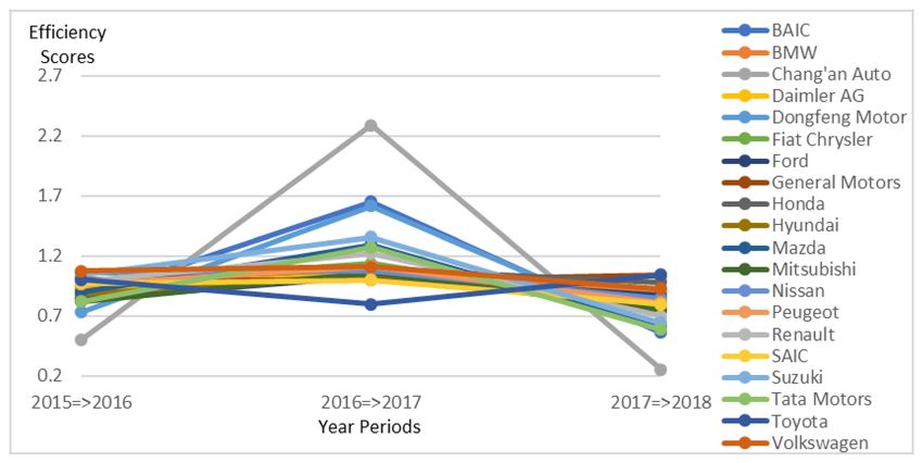
Mathematics 2020, 8, 580                                                                              3 of 21

model. Research procedures and discussions regarding the theory of the Malmquist index model, as
well as the Pearson correlation coefficient, are presented in the third section. The fourth section presents
the data and calculation, analysis, and evaluation. The last section of this research discusses the
conclusion contributions, shortcomings of research, and indicates some direction for the next research.

2. Literature Review
      In 1978, Charnes et al. [3] developed Data Envelopment Analysis (DEA). During that time, DEA
was a new data-oriented method for the evaluation of Decision-Making Units (DMUs). DMUs is a
set of peer entities in which technical efficiencies are calculated. It is a method of optimization with
the use of linear programming that will assess the productivity and efficiency of DMUs related to
the proportional change in inputs or outputs. The CCR is the first DEA model and is an acronym
for Charnes, Cooper, and Rhodes. Then, later, several models of DEA were introduced and broadly
applied for performance analysis in many areas, like transportation, mining, logistics, banking, and
many other industries and organizations since then. DEA was also used by Martín and Roman [4]
in 2001, wherein the performance and technical efficiencies of each individual airports in Spain are
analyzed. The results were used to set forth some considerations to the policies that prepare the
Spanish airport for the privatization process in 2001. Kulshreshtha et al. [5] utilized DEA to study
the productivity of the coal industry of India during the period of 1985–1997 and found that the
underground mining has less efficiency than the opencast mining. Leachman [6] used DEA for the
development of a quality and output-based performance metric to assess the competitiveness of car
firm’s manufacturing against its competitors. Pilyavsky et al. [7] deployed DEA to analyze the change
in efficiency of 193 community hospitals and polyclinics across the Ukraine, in the 1997–2001 period,
and found that the polyclinics somewhat less efficient than community hospitals. Wang et al. [8], in
their study, used DEA for the measurement of the marketing and production efficiencies of some
23 companies involved in the Printing Circuit Board (PCB) industry and found that 15 firms need
to improve their efficiencies in both production and marketing aspects. Four companies prioritized
the progress in their production efficiency, and the remaining four companies focused on enhancing
marketing efficiency. Chandraprakaikul and Suebpongsakorn [9], by deploying DEA, found out the
weaknesses of 55 logistic firms in Thailand. The goal of their study was to improve the logistics
efficiency and evaluate each firm’s performances from 2007 to 2010. An application of a DEA with
two-stage method was used by Yuan and Tian [10], to analyze the efficiency of resources related to
science and technology aspects of several industrial enterprises, along with other factors influencing
their performance. Findings show that the elements of the input and output variables are independent.
Chang et al. [11] analyzed the environmental efficiency of the transportation sector in China, by using
the DEA model to find out the very inefficient environment of the industry. Ren, et al. [12] applied
DEA for the assessment of six Chinese biofuel firms’ energy efficiency in relation to their life cycle,
to determine wasteful energy losses in biofuel production, and indicated that DEA is a feasible and
unique tool for establishing efficient scenarios in production of bioethanol. The research also suggested
that the most energy-efficient form of ethanol production for China may come from sweet potatoes.
DEA has been acknowledged as a practical decision support tool and a valuable analytical research
instrument. From a series of the previous studies mentioned above, it is understood that the DEA
method has been broadly applied to assess the performance of many companies in different industries,
including the automotive industry. These prove that DEA is an effective tool for the authors to evaluate
the performance of global automobile manufacturers.
      Malmquist productivity index (MPI) is a very useful approach for productivity measurement
in DEA. In 1982, Caves introduced MPI and named it after Professor Malmquist (1953), whom the
ideas are based upon. The Malmquist productivity index has the components which are used in
performance measurement that includes the technical efficiency in technological change and the total
factor productivity [13].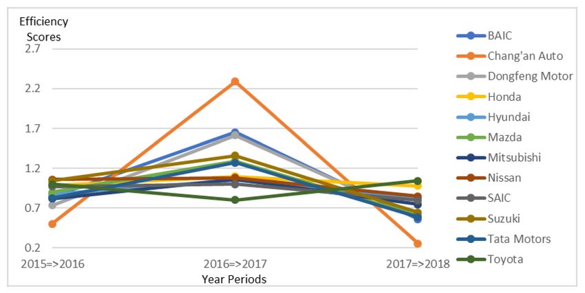
Mathematics 2020, 8, 580                                                                             4 of 21

      As stated in a study by Fuentes and Bañuls, [14] the split of the MPI’s Total Productivity Efficiency
into two different components, the technical efficiency and the technological, change helps clarify
the role of manager or skill level in the final performance data. The DEA Malmquist model has
been a very effective method in measuring changes in DMU productivity over the past decade.
For example, Färe, et al. [15] used it to analyze productivity growth in developed countries and found
that productivity growth in the United States was slightly above average, due to technological changes.
The growth in productivity of Japan turned out to be the highest among the samples, and because of
the changes in efficiency, Japan’s productivity growth is almost half. Fulginiti and Perrin [16] used
Malmquist to determine whether the results using this approach can confirm the recorded decline
in agricultural productivity from less-developed countries (LDCs) using other methods. The earlier
results were confirmed, and we found out that agricultural tax gets the most declining rates in terms
of productivity change. Odeck [17] focused on the Norwegian Motor Vehicle Inspection Agencies
and measured their efficiency and productivity growth for the period of 1989–1991. Using the
Malmquist index, the productivity was described through calculation by DEA, being the ratio between
efficiency for the similar production unit in two particular periods. The remarkably positive effect
of the frontier technology is observed to be the main contributor to the total productivity growth.
The efficiency measures that were calculated show that there are unstable efficiency scores for every
unit examined throughout the observed year periods. The size of the units does not have an effects
on the efficiency scores. Chen [18] used a non-radial Malmquist productivity index for the change
in productivity calculation of three major industries in China: chemicals, textiles, and metallurgical
within the four five-year plan periods. The research showed that the economic development plans
can be used for the evaluation of productivity and technology changes, using the MPI. Sharma [19]
examined the productivity performance of the Indian automobile industry via Total Factor Productivity
(TFP) measurement from 1990–1991 to 2003–2004 and explored further the factors influencing the
car industry efficiency in India. DEA was also used by Liu and Wang [20] to calculate the three
components of Malmquist productivity of some Taiwanese semiconductor packaging and testing
firms during the period of 2000 to 2003. Aside from revealing the productivity change patterns
and introducing another way to interpret the components of MPI with respect to management
aspects, this approach likewise determines any strategic shift of each firm due to isoquant changes.
Mazumdar [21] applied MPI to examine the technological gap ratio (TGR), technical efficiency, and
change in productivity of pharmaceutical companies among particular sectors in India. The study
implies that vertically integrated companies that produce both formulation and bulk drugs exhibit
higher efficiency and technological innovation, and it also found that imported technology or the
establishment of capital-intensive techniques propels the technological growth of firms.
      Wang et al. [22] compared the results of Malmquist productivity index to the Grey Relational
Analysis, to assess the intellectual capital management of the pharmaceutical industry in Taiwan. With
the combination of these analysis tools, they were able to conclude that, among the 12 pharmaceutical
companies, seven of them have efficiently improved their intellectual capital management, while five
companies failed during the four-year period of 2005 to 2008. Chang et al. [23] used the Malmquist
DEA model to study the productivity changes of accounting firms in the US, right before and after the
implementation of the Sarbanes–Oxley Act. The findings indicated that accounting firms exhibited
significant growth in productivity efficiency after the actualization of SOX, and these results were
better than pre-SOX performances.
      These studies cited above prove that the Malmquist productivity index (MPI), which is a
DEA-based model, is a very useful tool for measuring the productivity changes of countries, industries,
or organizations, through a specific assessment of technical and technological aspects, as well as total
factor productivity. Regarding this research, the authors know that car production is a complex activity
that combines technical aspects and technological capabilities; therefore, evaluating the performance
of an automobile manufacturer not only needs to include an evaluation of overall performance, but
it also needs to have specific technical and technological assessments. This Malmquist model is an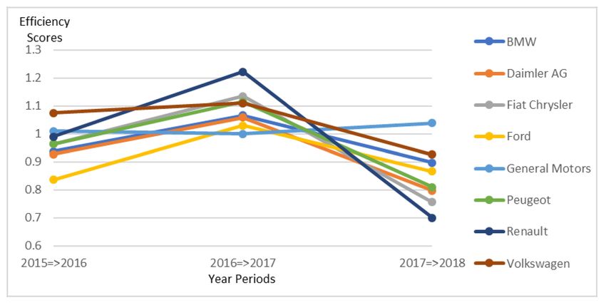
Mathematics 2020, 8, 580                                                                             5 of 21

appropriate research method to perform the most detailed evaluation of the technical, as well as the
technological, performance of global automakers. For this reason, the authors chose to apply this
Malmquist model to carry out this research.

3. Materials and Methods

3.1. Research Process
     In this research, the authors deployed the Malmquist productivity index model in the DEA
method, to evaluate the performance of the world’s top 20 automakers from 2015 to 2018. The study
includes four parts of processes, as shown in Figure 1.

                                     Figure 1. Procedures of research.

      Part 1. Literature review: The authors identified the research topic and method, and then learned
about the history of studies, using the selected method and the research that is related to the topic, in
order to have a research base for conducting this research.
      Part 2. Data collection: In this part, the authors selected the research objects, which are called
Decision Making Units (DMUs) in the DEA method. These DMUs are the world’s 20 largest automakers
by volume in 2015. Then, the choosing of appropriate input and output variables was done, to complete
the research data.
      Part 3. Data analysis: The collected data were checked for the correlation coefficient, to ensure the
relationship between input and output variables follows the isotonicity condition. If their correlation
coefficients are zero or negative, the data were re-selected, until they met the positive correlation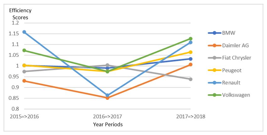
Mathematics 2020, 8, 580 6 of 21
coefficient requirement. After that, the DEA Malmquist model was applied, to calculate the catch-up
index, frontier-shift, and Malmquist index of the DMUs.
Part 4. Results, discussion: In the last part, the results of catch-up index (efficiency change),
frontier-shift (technological change), and Malmquist index (total factor productivity change) of the
DMUs are evaluated, discussed, and concluded.
3.2. Malmquist Productivity Index
Evaluating the change in total factor productivity of a DMU within two periods is the main
purpose of the MPI, being described as the product of catch-up efficiency change and technological
change (frontier-shift). Efficiency change is associated with the intensity of attempts of the DMU to
achieve any improvements or deterioration in its efficiency, while technological change reflects any
changes in the frontiers’ efficiency between the periods 1 to 2 [15].
The authors denote that the DMUi at the time period 1 is x1i , y1i and at the time period 2 is x2i , y2i .
t1
is measured by the technological frontier t2 : dt2 (xi, yi)t1
The efficiency score of the DMUi x1i , y1i
(t1 = 1, 2 and t2 = 1, 2).
To calculate for the catch-up (C), frontier-shift (F), and Malmquist Index (MI), the following
formulas can be used [8]:
d2 ((xi , yi )2 )
C= (1)
d1 ((xi , yi )1 )
1
d ((xi , yi )1 ) d1 ((xi , yi )2 ) 2
1
F = x 2
(2)
d2 ((xi , yi )1 ) d2 ((xi , yi ) )
1
d ((xi , yi )1 ) d1 ((xi , yi )2 ) 2
d2 ((xi , yi )2 )
1
MI = C x F = x x 2
(3)
d1 ((xi , yi )1 ) d2 ((xi , yi )1 ) d2 ((xi , yi ) )
1
d ((xi , yi )2 ) d2 ((xi , yi )2 ) 2
1
MI = x (4)
d1 ((xi , yi )1 ) d2 ((xi , yi )1 )
From the above formulas, we can see that the DMU’s total factor productivity (TFP) reflects the
advances or declines of the DMUs in technical and technological innovation efficiency. If the values
of C, F, and MI are >1, =0, or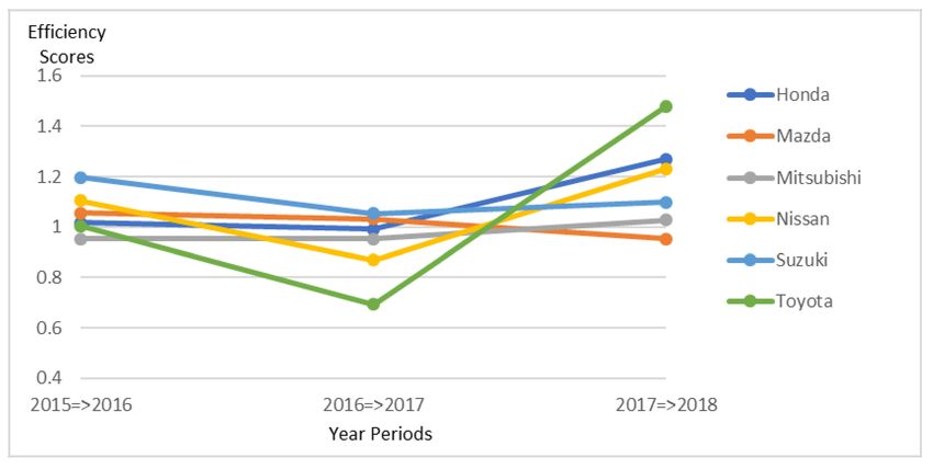
Mathematics 2020, 8, 580                                                                                7 of 21

                                    Figure 2. Linear correlation diagrams.

     Since the homogeneity and isotonicity are two important DEA data assumptions, these make the
correlation test an essential procedure before the application of DEA. This is an assurance that there is
an isotonic condition between input and output variables. The input and output data need to have a
positive correlation (the values of the output factors should not decrease while the values of the input
factors increase); the closer the value to +1, the better positive linear relationship.

3.4. Data Collection

3.4.1. Selection of Decision-Making Units (DMUs)
    This study focuses on the performance evaluation of the world’s top 20 automakers in terms of
production in 2015. They are the 20 automobile manufacturers (of more than 100 global automobile
manufacturers) that have a big impact on the global automotive industry, with an annual output of
over 1 million units. Out of these 20 automakers, there are 12 from Asia (six from Japan, four from
China, one from Korea, and one from India), six from Europe (three from Germany, two from France,
and one from the Netherlands), and two from the United States, as listed in Table 1, below.

      Table 1. List of 20 global automakers, according to the International Organization of Automobile
      Manufacturers (OICA) [24].

                                                               Production in 2015   Rank by Productions in
      DMUs            Automakers          Headquarters
                                                                    (Cars)                  2015
        D1              BAIC              Beijing, China             1,169,894               19
        D2              BMW           München, Germany               2,279,503               12
        D3         Chang’an Auto       Chongqing, China             1,540,133                16
        D4          Daimler AG         Stuttgart, Germany           2,134,645                14
        D5         Dongfeng Motor     Wuhan, Hubei, China            1,209,296               18
        D6          Fiat Chrysler    Amsterdam, Netherlands         4,865,233                 7
        D7               Ford             Michigan, US              6,396,369                 5
        D8         General Motors         Michigan, US              7,485,587                 4
        D9             Honda              Tokyo, Japan               4,543,838                8
        D10           Hyundai          Seoul, South Korea            7,988,479                3
        D11            Mazda            Hiroshima, Japan            1,540,576                15
        D12           Mitsubishi          Tokyo, Japan               1,218,853               17
        D13            Nissan           Yokohama, Japan             5,170,074                 6
        D14            Peugeot          Sochaux, France              2,982,035               11
        D15            Renault          Boulogne, France             3,032,652               10
        D16             SAIC            Shanghai, China              2,260,579               13
        D17            Suzuki          Hamamatsu, Japan             3,034,081                9
        D18          Tata Motors         Mumbai, India              1,009,369                20
        D19            Toyota              Aichi, Japan             10,083,831                1
        D20         Volkswagen        Wolfsburg, Germany             9,872,424                2

3.4.2. Selection of Input/Output Variables
    Selecting input and output factors is an important task in employing DEA to measure the efficiency
of DMUs. DEA is a complicated technique, wherein that the inputs and outputs have a strong impact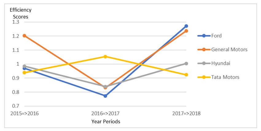
Mathematics 2020, 8, 580                                                                                 8 of 21

on the result. Based from inadequate benefit analysis, determination of the proper number of variables
can be neglected. Moreover, currently, there is no precise method in variable selection that must be
followed. According to previous studies, the authors found that input variables are financial indicators
that the company needs to balance or decrease, while output variables are indicators that the company
needs to improve or increase. After thorough study, the researchers decided to choose four input and
two output factors, which are stated below:
      Input Factors

1.    Total Assets (TA): the total amount of assets owned by the automaker second item.
2.    Equity (EQ): the higher the equity level of a company, the better access to many debt-based
      funding. If most assets come from equity, the financial leverage is low, and then equity can be a
      proxy for financial debt-based assets for companies.
3.    Cost of Revenue (CR): the total costs that are directly connected with producing and distributing
      goods and services to customers of the automaker.
4.    Operating Expenses (OE): expenditures incurred in carrying out automaker’s day-to-day activities
      but not directly associated with production, including selling, administrative and general expenses.

      Output Factors

1.    Revenue (RE): the total receipts that the automaker obtains from selling goods or services.
2.    Net Income (NI): the actual profit of the automaker after accounting for all costs, and taxes.

     These six important financial indicators play an important role in assessing a company’s
performance. Every business needs to manage its assets, control its capital well, reduce production and
operation costs, and increase its income and profits. The authors limited the input variables to only
financial indicators, since the study focused on the aspect of efficiency in terms of financial capabilities.
To be able to use these data for the DEA analysis, the authors chose the outputs which are necessarily to
be increasing along with the values of the input factors. There must be an isotonic condition between
the input and output variables, or else the chosen factors cannot be used. That is the reason why the
authors chose these factors as research variables.

3.4.3. Research Data
     The 2015–2018 period’s data were collected from the automobile manufacturers’ annual reports
and from information published on their official websites [25]. The unit is calculated in millions of US
dollars. Table 2 below shows the statistical data for each year period.

                              Table 2. Summary of statistics for each year periods.

     Year        Statistics     TA            EQ             CR            OE           RE          NI
     2015           Max        433,120      152,342        201,230       39,429        247,137     21,259
                    Min        13,412.1     5157.75        8011.05       1491.45       10,015.8     1.000
                    Ave.      134,650.3    36,800.74      75,644.54     12,096.33     92,420.68   5748.965
                    SD        123,220.5    36,012.59       58,281.8     9110.951      70,048.78   4687.882
     2016           Max        459,637      151,968        205,131       36,648        257,741     20,986
                    Min         13,010        6024          9673.2       1522.8        11,781.3      658
                    Ave.      142,609.1    38,525.88       78,302.2     13,096.46     97,175.87   4616.053
                    SD        129,059.5    36,322.72      58,893.88     9264.601      72,236.68   4603.454
     2017           Max        473,616      158,936        211,055       32,643        258,779     20,481
                    Min         13,470       6125.4       10,404.45      1539.3        12,001.8     1.000
                    Ave.      148,300.6    41,408.17       80,085.3     12,902.93     99,035.85   8459.098
                    SD        132,444.6    39,474.08      60,039.49     8548.417      72,817.91   5008.035
     2018           Max        513,959      170,017        216,779       35,803        266,601     22,631
                    Min       14,023.35     6936.75        8487.45       1302.3         9944.7     102.15
                    Ave.      156,200.6    44,524.12      83,214.39     13,574.66     102,395.2   5283.818
                    SD        140,497.7    41,682.19      61,858.42     9347.215      75,298.09   5322.953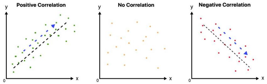
Mathematics 2020, 8, 580                                                                                  9 of 21

     D20 in 2015, and D8 and D12 in 2017 have negative values in Net Income (this is an indication that
those firms suffered a loss during that year). Since homogeneity is an important aspect of DEA data
assumption, the negative values from the raw data need to be adjusted upward, to positive values.
After adjustment, the net income of each DMU in 2015 increased by 1538, and in 2017, increased by
3865. This simultaneous change of value does not affect the DEA calculation results.
     The process, methods, tools, and research data to carry out this study were discussed above. In the
next section, the authors apply the Pearson correlation coefficient testing tool and DEA Malmquist
model, to calculate the research data.

4. Results and Discussion

4.1. Correlation Results
     In DEA, a variable is a factor that greatly affects the research results. Before using the Malmquist
or any model in DEA to process the data, the isotonic condition in between the input and output
variables must be met. It only means that the increase in the values of the input variables should
not make the values of the output variables decrease [26]. Therefore, the research data must first be
validated by using the Pearson correlation, to ensure the isotonic relationship between input and
output variables. The value range of the Pearson correlation coefficient is from −1 to +1. The results of
the Pearson correlation test are shown in Table 3, below.

                              Table 3. Coefficients of correlation between variables.

                Factors            TA           EQ               CR             OE       RE       NI
                                                         2015
            Total Assets         1.0000        0.9256           0.9556         0.9017   0.9666   0.6036
               Equity            0.9256        1.0000           0.8440         0.7933   0.8670   0.6986
          Cost of Revenue        0.9556        0.8440           1.0000         0.9070   0.9972   0.5770
         Operating Expenses      0.9017        0.7933           0.9070         1.0000   0.9165   0.3494
             Revenue             0.9666        0.8670           0.9972         0.9165   1.0000   0.6034
            Net Income           0.6036        0.6986           0.5770         0.3494   0.6034   1.0000
                                                         2016
            Total Assets         1.0000        0.9213           0.9507         0.9063   0.9583   0.7981
               Equity            0.9213        1.0000           0.8626         0.8061   0.8783   0.8778
          Cost of Revenue        0.9507        0.8626           1.0000         0.9227   0.9984   0.7835
         Operating Expenses      0.9063        0.8061           0.9227         1.0000   0.9342   0.6172
             Revenue             0.9583        0.8783           0.9984         0.9342   1.0000   0.7952
            Net Income           0.7981        0.8778           0.7835         0.6172   0.7952   1.0000
                                                         2017
            Total Assets         1.0000        0.9305           0.9554         0.9185   0.9610   0.8320
               Equity            0.9305        1.0000           0.8736         0.8142   0.8785   0.8651
          Cost of Revenue        0.9554        0.8736           1.0000         0.9374   0.9987   0.7928
         Operating Expenses      0.9185        0.8142           0.9374         1.0000   0.9506   0.6963
             Revenue             0.9610        0.8785           0.9987         0.9506   1.0000   0.7915
            Net Income           0.8320        0.8651           0.7928         0.6963   0.7915   1.0000
                                                         2018
            Total Assets         1.0000        0.9258           0.9476         0.9059   0.9551   0.8739
               Equity            0.9258        1.0000           0.8748         0.8093   0.8866   0.9429
          Cost of Revenue        0.9476        0.8748           1.0000         0.9341   0.9985   0.8730
         Operating Expenses      0.9059        0.8093           0.9341         1.0000   0.9460   0.7973
             Revenue             0.9551        0.8866           0.9985         0.9460   1.0000   0.8841
            Net Income           0.8739        0.9429           0.8730         0.7973   0.8841   1.0000
                                          Source: calculated by researchers.

     The correlation coefficient ranges from 0.3494379 to 1; all are positive correlations. It means that
the used data comply with isotropic conditions and can be used for DEA calculations. This also proves
that the choice of inputs and outputs is applicable for DEA.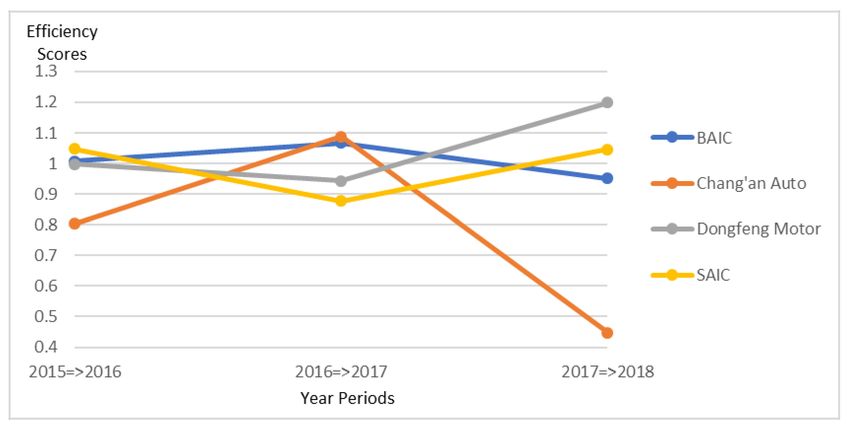
Mathematics 2020, 8, 580                                                                                     10 of 21

4.2. Catch-Up Index (Technical Efficiency)
     The Malmquist productivity index has the components which are used in performance
measurement, such as changes in technical, technological, and total factor productivity. The authors
present results of efficiency change. The technical effective changes of the DMUs are expressed through
the catch-up index shown in the Table 4 and Figure 3.

                                     Table 4. Result of the DMUs’ catch-up index.

         DMUs                Automaker        2015 ≥ 2016        2016 ≥ 2017     2017 ≥ 2018    Average
          D1                    BAIC          1.007906519        1.067588827     0.951099081   1.008864809
          D2                    BMW           1.002200700        0.989942896     1.032516308   1.008219968
          D3               Chang’an Auto      0.802806822        1.088698475     0.447817244   0.779774180
          D4                Daimler AG        0.930637488        0.851411104     1.006351466   0.929466686
          D5               Dongfeng Motor     0.997491449        0.942585562     1.198699708   1.046258907
          D6                Fiat Chrysler     0.974202762        1.003801147      0.93822297   0.972075626
          D7                     Ford         0.969533267        0.772186068     1.272174794   1.004631376
          D8               General Motors     1.203162859        0.831481843     1.238505175   1.091049959
          D9                   Honda          1.017930963        0.991968224     1.268988397   1.092962528
          D10                 Hyundai         0.985207492        0.839423806     1.003855082   0.942828794
          D11                  Mazda          1.056287293        1.032101748     0.951842778   1.013410606
          D12                 Mitsubishi      0.952867583        0.951779377     1.027294947   0.977313969
          D13                  Nissan         1.103923082        0.869170202     1.230991107    1.06802813
          D14                  Peugeot        1.002611318         0.97492581     1.064404376   1.013980502
          D15                  Renault        1.157947517        0.863096113     1.109919469   1.043654366
          D16                   SAIC          1.048487305        0.876499742     1.046332557   0.990439868
          D17                  Suzuki         1.197202876        1.053332401     1.097676298   1.116070525
          D18                Tata Motors      0.939140968        1.053801742     0.923920449   0.972287719
          D19                  Toyota         1.004901805        0.692280752     1.479811835   1.058998131
          D20               Volkswagen         1.07190144          0.974113       1.12718749   1.057733977
        Average                               1.021317575        0.936009442     1.070880577   1.009402531
         Max                                  1.203162859        1.088698475     1.479811835   1.116070525
         Min                                  0.802806822        0.692280752     0.447817244    0.77977418
                                            Source: calculated by researchers.

                                  Figure 3. Technical efficiency changes of each DMU.

      Catch-up index, with scores >1 and 1) reflects that the majority
(13 DMUs: D1, 2, 5, 7, 8, 9, 11, 13, 14, 15„17, 19, and 20) achieved technical efficiency in the total
Mathematics 2020, 8, 580 11 of 21
research period (2015–2018). D17 (Suzuki) achieved the best and the most stable technical performance,
while D3 (Chang’an Auto) had the lowest and the least-stable efficiency performance on average.
During the 2015–2016 period, 12 of the 20 DMUs achieved technical efficiency, with the catch-up
index greater than 1. The DMU that had the highest technical efficiency was D8 (General Motors), with
a value of 1.203. Meanwhile, D3 had the lowest technical efficiency, at 0.779774180
It is noticeable that, during the period of 2016–2017, most of the DMUs did not achieve progressive
technical efficiency (D1, 3, 6, 11, 17, and 18), with catch-up scores greater than 1. D19 (Toyota) was
the least-efficient automobile manufacturer in this period, with a score of 0.692. D3 (Chang’an Auto)
had an impressive improvement in technical efficiency, being the least-effective producer during the
previous period and then becoming the most technically efficient producer in this period.
After the low performance from the previous period, the automakers showed significant
improvement in technical efficiency in the next period, 2017–2018. Results show that there are
only five out of 20 companies (D1, 3, 6, 11, and 18) that have catch-up values less than 1. Being
the worst-performing manufacturer in the previous period, D19 (Toyota) had shown improvement
and became the most technically efficient manufacturer in this period, with a catch-up value of 1.47.
Surprisingly, D3 (Chang’an Auto) failed to maintain high efficiency and suffered a serious decline in
technical efficiency, with a catch-up value of only 0.4478, while the other competitors were above 0.9.
In the list of 20 DMUs, four of them are from China, six from Japan, six from Europe, two
from America, one from Korea, and one from India. Among the four Chinese carmakers (D1-BAIC,
D3-Chang’an Auto, D5-Dongfeng, and D16-SAIC), the authors noticed, in Figure 4 below, that Dongfeng
and SAIC showed improvement in technical efficiency, while Chang’an Auto and BAIC regressed in
regard to efficiency change.
Figure 4. Technical-efficiency changes of Chinese automakers.
After a decline in technical efficiency during the period of 2016–2017, except for Mazda (D11), the
remaining five Japanese automakers had a clear improvement, as seen in Figure 5, below. Toyota (D19)
showed the most noticeable improvement, by going from being the least-effective manufacturer to
becoming superior compared to other competitors.Mathematics 2020, 8, 580 12 of 21
Figure 5. Technical-efficiency changes of Japanese automakers.
Like Japanese automakers, European carmakers also tended to improve their performances after
the previous decline. Only one automaker, Fiat Chrysler (D6), showed a degradation in technical
efficiency, as seen in Figure 6.
Figure 6. Technical-efficiency changes of European automakers.
Figure 7, below, shows the remaining four manufacturers, Ford, General Motor (from the
US), Hyundai (from Korea), and Tata Motors (from India) exhibiting less-significant changes in
technical efficiencies.
Despite being less effective than its rival, General Motors (D8), in previous periods, Ford (D7)
showed improvement in technical efficiency and even surpassed its rival during the 2017–2018 period.
The Korean automaker Hyundai (D10) improved its technical efficiency, and the Indian automaker Tata
Motors (D18) showed a regress, despite achieving good performance in the previous 2016–2017 period.Mathematics 2020, 8, 580 13 of 21
Figure 7. Technical-efficiency changes of US, Korean, and Indian automakers.
4.3. Frontier-Shift Index (Technological Change)
The frontier-shift index is applied to measure the efficiency frontiers of DMUs between two
periods. Table 5 shows that the technological efficiency of automobile manufacturers increased in the
period 2016–2017 and decreased in the period of 2017–2018.
Table 5. Frontier-shift index of the DMUs.
DMUs Automaker 2015 ≥ 2016 2016 ≥ 2017 2017 ≥ 2018 Average
D1 BAIC 0.836805193 1.546229001 0.588987818 0.990674
D2 BMW 0.934837626 1.076482507 0.868562222 0.9599608
D3 Chang’an Auto 0.620779568 2.104430625 0.566303729 1.0971713
D4 Daimler AG 0.996127981 1.243645099 0.791735446 1.0105028
D5 Dongfeng Motor 0.733741954 1.711266889 0.488457455 0.9778221
D6 Fiat Chrysler 0.98892349 1.130289028 0.805868394 0.975027
D7 Ford 0.861670304 1.333023477 0.681088404 0.9585941
D8 General Motors 0.838888086 1.202999181 0.838415742 0.960101
D9 Honda 0.967083237 1.106332753 0.771206593 0.9482075
D10 Hyundai 0.892240838 1.249043339 0.813506803 0.9849303
D11 Mazda 0.850399789 1.2533984 0.634128384 0.9126422
D12 Mitsubishi 0.859881874 1.112169071 0.725179558 0.8990768
D13 Nissan 0.959916617 1.241455916 0.687654242 0.9630089
D14 Peugeot 0.961643757 1.14347053 0.761186141 0.9554335
D15 Renault 0.855171144 1.416545764 0.630590472 0.9674358
D16 SAIC 0.925493158 1.141159707 0.761752174 0.9428017
D17 Suzuki 0.87126208 1.28910142 0.585370558 0.9152447
D18 Tata Motors 0.873868983 1.205930386 0.635285567 0.9050283
D19 Toyota 0.996099676 1.154084768 0.703886497 0.951357
D20 Volkswagen 1.003309415 1.139756648 0.821471088 0.9881791
Average 0.891407239 1.290040725 0.708031865 0.9631599
Max 1.003309415 2.104430625 0.868562222 1.0971713
Min 0.620779568 1.076482507 0.488457455 0.8990768
Source: calculated by researchers.
Except for D20, the remaining all of the manufacturers (19 out of 20) failed to achieve technological
progress in the first period of 2015–2016. However, in the next period (2016–2017), manufacturers
made efforts in innovating technology and achieving good results. However, they were not able to
maintain this progress in the next period (2017–2018), as all of their frontier-shift indicators were
lower than 1, even lower than the 2015–2016 period. This shows that the frontier-shift efficienciesMathematics 2020, 8, 580 14 of 21
of manufacturers seriously fell down during this period. Due to the low value of technological
efficiencies in the periods 2015–2016 and 2017–2018, except for Chang’an Auto (D3) and Daimler AG
(D4), the average technological efficiency during the total research period (2015–2018) did not result in
a progressive score.
It can be observed in Figure 8 that the automobile manufacturers did not achieve technological
progress during the period of 2015–2016. Only D20 (Volkswagen) obtained a frontier-shift index greater
than 1, indicating that the development in technology and innovation of the global auto industry have
not improved very well and have many limitations. After a period of poor technological performance
2015–2016, manufacturers opted to invest in technology innovation and achieved technological
efficiency in the period 2016–2017, especially D1, D3, D5, D7, D10, D11, D15, and D17. However,
because technology development has been so fast and developing, manufacturers failed to maintain
progress and even severely declined in the next period.
Figure 8. Technical-efficiency frontier of the DMUs.
Figure 9, below, shows the frontier-shift scores of automobile manufacturers in the period of
2017–2018. During this period, the manufacturers with low efficiencies (F < 0.6) were Dongfeng,
Chang’an Auto, BAIC (manufacturers from China), and Suzuki (Japan). Manufacturers such as Renault,
Mazda, Tata Motors, Ford, and Nissan also had a low performance (F < 0.7). BMW, General Motors,
Volkswagen, Hyundai, and Fiat Chrysler had better technological efficiency than the rest, with F > 0.8.
Thus, it can be seen that, in this period, manufacturers from Asia, especially China, had a more
serious decline in technological efficiency than European and American automobile manufacturers.
The simultaneous decline in technological efficiency of all 20 automobile manufacturers shows a close
correlation with the decline in global automobile production in this period of 2017–2018.
In terms of technological efficiency, it can be seen that the automakers show a common
trend, increasing in the second phase and declining in the remaining two periods, showing that
no manufacturer performed a stable technological efficiency or took any lead in the race to technology
development and innovation. It only shows that the technology playground in the global automotive
industry is highly competitive and holds so much potential for all manufacturers.Mathematics 2020, 8, 580 15 of 21
Figure 9. Frontier-shift index of automakers in 2017–2018 period.
4.4. Malmquist Productivity Index (MPI)
MPI is one very valuable component in evaluating the performance of global automobile
manufacturers. It measures the change in total factor productivity of DMUs at a certain interval periods
and is the product of catch-up index (technical efficiency) and frontier-shift (technological change).
As shown in Table 6 and Figure 10, the average Malmquist index of DMUs less than 1 (0.9632678)
indicates a regression in the total productivity growth of the DMUs. The total performance of most
DMUs increased in the period 2016–2017 and significantly decreased in the 2017–2018 period.
Table 6. Malmquist productivity index of the DMUs, from 2015 to 2018.
DMUs Automaker 2015 ≥ 2016 2016 ≥ 2017 2017 ≥ 2018 Average
D1 BAIC 0.84342141 1.650736804 0.560185773 1.0181147
D2 BMW 0.936894924 1.06565621 0.896804659 0.9664519
D3 Chang’an Auto 0.498366072 2.291090413 0.253600576 1.0143524
D4 Daimler AG 0.927034042 1.058853247 0.796764127 0.9275505
D5 Dongfeng Motor 0.731901325 1.613015462 0.585513808 0.9768102
D6 Fiat Chrysler 0.963411995 1.134585423 0.756084238 0.9513606
D7 Ford 0.835418025 1.029342158 0.8664635 0.9104079
D8 General Motors 1.009318988 1.000271976 1.038382236 1.0159911
D9 Honda 0.984423971 1.097446936 0.978652219 1.0201744
D10 Hyundai 0.879042358 1.048476714 0.816642939 0.9147207
D11 Mazda 0.898266491 1.293634679 0.603590522 0.9318306
D12 Mitsubishi 0.819353562 1.058539585 0.744973296 0.8742888
D13 Nissan 1.05967411 1.079036489 0.846496257 0.995069
D14 Peugeot 0.964154915 1.114798933 0.81020986 0.9630546
D15 Renault 0.990243303 1.222615142 0.699904642 0.970921
D16 SAIC 0.970367828 1.000226189 0.797046101 0.9225467
D17 Suzuki 1.043077467 1.357852294 0.642547387 1.0144924
D18 Tata Motors 0.820686163 1.270811541 0.586953327 0.892817
D19 Toyota 1.000982362 0.798950672 1.04161957 0.9471842
D20 Volkswagen 1.075448807 1.110251768 0.925951934 1.0372175
Average 0.912574406 1.214809632 0.762419348 0.9632678
Max 1.075448807 2.291090413 1.04161957 1.0372175
Min 0.498366072 0.798950672 0.253600576 0.8742888
Source: calculated by researchers.Mathematics 2020, 8, 580 16 of 21
Figure 10. Total-factor-productivity change.
In the period of 2015–2016, most of the DMUs performed inefficiently, with the MPI less than
1, only five automakers, namely General Motors (G.M.), Nissan, Suzuki, Toyota, and Volkswagen,
achieved progress in total factor productivity.
After performing low efficiency in the 2015–2016 period, car producers improved their productivity
and got a good performance. This can be seen by the positive MPI values of DMUs in the next period,
2016–2017. Only D19 (Toyota) did not achieve an efficient performance during this period, with an
MPI of 0.7989.
However, the manufacturers could not maintain this progressive performance for the next period,
2017–2018. The productivity scores of automakers even declined very badly, having an average value
of only 0.762. The lowest index of 0.2536 belongs to D3 (Chang’an Auto), meaning that it was the
least-efficient producer at this period. The two occasional outstanding automakers that achieved a
good performance in this period were D8 (General Motors) and D19 (Toyota), with the MPI equal to
1.0383 and 1.0416, respectively.
Although DMUs had a great improvement and performance in the period 2016–2017, the
performance in the other two periods were poor (especially in the 2017–2018 period), resulting in 14
out of 20 DMUs having a low-efficiency performance during the research period of 2015–2018 (total
average MPI less than 1). Among 20 automotive manufacturers, General Motors is the automaker
that had the most stable performance in all stages (all MPI values were greater than 1). Despite the
inefficient performance in the 2017–2018 period, Volkswagen is still the best-performing automaker
in the total research period, with an average MPI value of 1.037. Volkswagen is followed by Honda,
BAIC, General Motor, Suzuki, and Chang’an Auto. In contrast, Mitsubishi and Tata Motors were the
worst-performing automakers, with the lowest average MPI values.
Figure 11 presents the total factor productivity change of Asian automakers over the research
period, 2015–2018. In the figure, there is a big difference in the performance between the Asian
manufacturers. Chinese manufacturers have the biggest fluctuation in performance. Among four
Chinese automakers, namely D1 (BAIC), D3 (Chang’an Auto), D5 (Dongfeng), and D16 (SAIC), SAIC
was more stable compared to others in terms of performance; the remaining automakers showed
big fluctuations, with performances that increased rapidly but fell drastically afterward. It can be
recognized that Chinese car manufacturers have still not improved the stability in production efficiency
and are still struggling to stabilize their production performance.Mathematics 2020, 8, 580 17 of 21
Figure 11. Total-factor-productivity change of Asian automakers.
For Japanese automakers, Toyota (D19) is the manufacturer with the best breakthrough from
the least-efficient manufacturer in the second phase to become the only manufacturer to achieve
progressive performance in the 2017–2018 period. Honda (D9) shows a stable performance compared
to other Japanese companies and other Asian manufacturers. In contrast, Mazda (D11) and Suzuki
(D17) need more stability in performance. The other two Asian car producers, Korea’s Hyundai (D10)
and India’s Tata Motors (D18), do not have a stable performance, especially in the 2017–2018 period.
The Indian automobile manufacturers demonstrated very poor performance during the 2017–2018
period, lagging behind the three Chinese automobile manufacturers.
As gleaned in Figure 12, there is no significant difference in total factor productivity between
the European and American automobile manufacturers. Thus, it can be seen that the performance
of European and American manufacturers does not have major fluctuations compared to Asian
manufacturers. During the first phase (2015–2016), only Volkswagen (D20) and General Motors (D8)
achieved the total factor productivity, while Ford (D7) was the least-efficient producer during this
period. Like the Asian companies, European–American automobile manufacturers showed increasing
growth in the year 2016–2017. All of the eight European–American manufacturers achieved total
factor productivity in this period. Unfortunately, only General Motors was able to maintain this good
performance up to the next period, 2017–2018. It is also noticeable that the most unstable manufacturer
in terms of performance is Renault (D15). This is due to the automaker’s progress on the second-phase
performance but fell sharply in the final stage. In contrast to Renault, General Motor is the most stable
producer in terms of performance; even when other manufacturers declined in performance, it not
only maintained, but also increased, in its performance.
In general, Honda is the only Asian automaker with the best performance, while Volkswagen and
General Motors are from Europe–America. Asian automobile manufacturers, especially Chinese
automakers, have made breakthrough performances during the 2016–2017 period, in terms of
productivity. However, since the productivity efficiencies are not stable, they lost the race in the
next period, 2017–2018. Thus, Asian manufacturers—China in particular—need to stabilize their
production performance, in order to compete with European manufacturers. Based on the technical,
as well as the technology, growth trend of the 20 automobile manufacturers, it can be seen that they
still have not balanced the technical efficiency and technological efficiency. Typically, in the period of
2016–2017, when they improved technological change, the technical efficiency regressed. Moreover, the
manufacturers were able to improve their technical efficiency, but they were faced with challenges in
the technological-innovation aspects, during the period of 2017–2018. Therefore, improving productionMathematics 2020, 8, 580 18 of 21
performance is about making a balance between technical efficiency and technological change; and
these two aspects can be developed simultaneously
Figure 12. Total-factor-productivity change of European–American automakers.
5. Conclusions
This study illustrates the results of technical efficiency, technological progress, and the total factor
productivity of automakers in the four-year periods. Findings show that, after a period of slight decline,
most manufacturers have gradually improved their technical efficiency, which somehow leads to
technical progress. Suzuki turned out to be the best and most stable manufacturer in terms of technical
efficiency, while Chang’an Auto needs more improvement in this aspect. In terms of technological
progress, most manufacturers have an unstable performance, especially the Chinese automakers. This
regress in performance is also noticed in the study conducted by Imran et al. [27] wherein the export
performance of Chinese automotive sector is the main scope. Exportation of automobile units affects
the revenue and income of the company in which this paper uses as variables.
Although automakers had a breakthrough in innovation and achievement, as they were able to
perform efficiently during the 2016–2017 period, this was not maintained, and they even had a big
regression of technological efficiency in the next period. It only affirms that the technology arena in the
global automotive industry is highly competitive and shows so much potential for all automakers, since
none of them is taking the lead. However, Fathali et al. [28] discussed that there is no strong empirical
and theoretical evidence that competition is a major driving force to improvement in technology and
innovation. Therefore, whatever the kind of competitive environment the automotive industry is in,
there will be continuing technological and innovative development.
Since the total factor productivity is the product of technical efficiency and technological efficiency,
manufacturers must balance the development to both technical and technological efficiency, to be able
to achieve a progressive outcome. Based on the results, only General Motors achieved a Malmquist
index greater than 1 in all year periods. This implies that this manufacturer is the best and most
stable automaker among the others. Mitsubishi and Tata Motors are the automakers with the lowest
performance on average. The results also show that there is less variation in total factor productivity
of European–American producers than Asian manufacturers. The year 2017–2018 is the period
when automobile output dropped suddenly after a phase of growth. It is also the period when the
technological efficiency index of all 20 automakers significantly declined compared to the previous
period, confirming the influence of technological changes to this fluctuation. Therefore, automobile
manufacturers need to focus on handling their technology and innovation properly, to avoid theMathematics 2020, 8, 580 19 of 21
occurrence of a second automobile crisis. This is not in reference to any oil crisis, but a possible industry
4.0 crisis.
This study applied the DEA Malmquist model to evaluate the performance of the world’s top 20
automakers over the period of 2015–2018, based on input and output variables, which are very important
financial indicators. Based on results, the performance of the world’s top 20 automobile manufacturers
in terms of technical efficiency, technological efficiency, and total factor productivity not only indicates
the overall picture of the world automobile industry but also provides a comparative performance of
manufacturers from different countries and continents. The study presented an overview of the Chinese,
Japanese, Asian, or European–American automobile industries. Therefore, this can be a valuable
reference for car managers, policy makers, or investors for automobile management, investment, and
development decisions. Moreover, this study can be used as a guide for automobile manufacturers to
form strategic alliance with one another. Wang et al. [29] strongly recommends that the manufacturers
in the automobile industry form a strategic alliance with one another, given that there will be an
extensive analysis of companies’ performances before forming one in which the DEA is a very effective
tool. In addition, the study also contributes to the application of the data envelopment analysis
method, specifically the Malmquist model in organizational performance measurement, and is a
worthy document for the studies of global automotive industry, as well as other fields.
However, the study has several limitations that must be considered. First, the results of this study
depend on the value of the input and output variables, which are financial in nature. The results
indicated in this study is not applicable or relatable to any other type of industry, even those that are
a little related to automobiles, such as the petroleum or fuel industry. However, this study can also
be an additional reference, like the other studies cited in this paper. For future studies, the authors
must make some modifications in the variables used and then compare the results, to provide a more
objective research result. It can also be recommended to improve this kind of study by integrating
several input and output factors, such as total number of units produced; undesirable outputs, such
as total number of defective units being recalled; and other non-financial variables. Eilert et al. [30]
described how the volume of recalled automotive products can somehow affect the sales of the firms, as
it may hurt their brand reliability and company’s reputation. Research and development expenditure
can also be a factor for future studies. Hashmi and Biesebroeck [31] pointed out that the industry
leader’s aspect of innovation is greatly declining in the efficiency of the automotive firms lagging
behind. They mentioned that highly focusing on efficiency leads to an increase in innovation. It will be
interesting to know the effects of R&D in the efficiency level of automotive firms. Second, this study
focuses on evaluation of the performance from the world’s 20 largest automakers. Involvement of other
automakers is recommended, in order to give a general overview of the industry performance. Finally,
this study is based on a quantitative approach, using DEA Malmquist model, where some external
factors are not being considered. The combination with qualitative research will be a worthwhile
research direction to more fully evaluate the performance of the automobile manufacturers.
Author Contributions: Conceptualization, C.-N.W., H.T., and H.A.N.; Data curation, H.T. and H.A.N.; Formal
analysis, H.T. and H.A.N.; Funding acquisition, C.-N.W.; Investigation, H.T. and H.A.N.; Methodology, C.-N.W.,
H.T., and H.A.N.; Project administration, C.-N.W.; Writing—Original draft, H.T. and H.A.N.; Writing—Review
and editing, C.-N.W. and H.T. All authors have read and agreed to the published version of the manuscript.
Funding: This research received no external funding.
Acknowledgments: The authors appreciate the support from Taiwan National Kaohsiung University of Science
and Technology, Philippines Technological University of the Philippines Taguig, and Taiwan Ministry of Sciences
and Technology.
Conflicts of Interest: The authors declare no conflict of interest.
References
1. Humphrey, J.; Memedovic, O. The global automotive industry value chain: What prospects for upgrading
by developing countries. In UNIDO Sectorial Studies Series Working Paper; UNIDO: Vienna, Austria, 2003.You can also read