Projections of Future Climate Change in Singapore Based on a Multi-Site Multivariate Downscaling Approach
←
→
Page content transcription
If your browser does not render page correctly, please read the page content below
water
Article
Projections of Future Climate Change in Singapore
Based on a Multi-Site Multivariate
Downscaling Approach
Xin Li 1, * , Ke Zhang 2, *       and Vladan Babovic 3
 1   College of Hydrology and Water Resources and CMA-HHU Joint Laboratory for HydroMeteorological
     Studies, Hohai University, Nanjing 210098, China
 2   State Key Laboratory of Hydrology-Water Resources and Hydraulic Engineering, CMA-HHU Joint
     Laboratory for HydroMeteorological Studies, and College of Hydrology and Water Resources,
     Hohai University, Nanjing 210098, China;
 3   Department of Civil and Environmental Engineering, National University of Singapore,
     Singapore 119077, Singapore; vladan@nus.edu.sg
 *   Correspondence: xinli@hhu.edu.cn (X.L.); kzhang@hhu.edu.cn (K.Z.);
     Tel.: +86-18851715807 (X.L.); +86-25-83787112 (K.Z.)

 Received: 26 September 2019; Accepted: 30 October 2019; Published: 3 November 2019

 Abstract: Estimates of the projected changes in precipitation and temperature have great significance
 for adaption planning in the context of climate change. To obtain the climate change information at
 regional or local scale, downscaling approaches are required to downscale the coarse global climate
 model (GCM) outputs to finer resolutions in both spatial and temporal dimensions. The multi-site,
 multi-variate downscaling approach has received considerable attention recently due to its advantage
 in providing distributed, physically coherent downscaled meteorological fields for subsequent impact
 modeling. In this study, a newly developed multi-site multivariate statistical downscaling approach
 based on empirical copula was applied to downscale grid-based, monthly precipitation, maximum
 and minimum temperature outputs from nine global climate models to site-specific, daily data over
 four weather stations in Singapore. The advantage of this approach lies in its ability to reflect the
 at-site statistics, inter-site and inter-variable dependencies, and temporal structure in the downscaled
 data. The downscaling was conducted for two projection periods (i.e., the 2021–2050 and 2071–2100
 periods) under two emission scenarios (i.e., representative concentration pathway (RCP)4.5 and
 RCP8.5 scenarios). Based on the downscaling results, projected changes in daily precipitation,
 maximum and minimum temperatures were examined. The results show that there is no consensus
 on the projected change in average precipitation over the two future periods. The major uncertainty
 for precipitation projection comes from the GCMs. For daily maximum and minimum temperatures,
 all downscaled GCMs project an increase of average temperature in the future. These change signals
 could be different from those of the original GCM data, both in magnitude and in direction. These
 findings could assist in adaption planning in Singapore in response to emerging climate risks.

 Keywords: multi-site multivariate downscaling; Empirical Copula; inter-site correlation;
 inter-variable dependence; temporal structure; Singapore

1. Introduction
     Estimates of the projected changes for the most relevant meteorological variables are essential
for stakeholders to anticipate adaptation strategies for emerging climate risks. General circulation
models (or global climate models) (GCMs) are often used to provide climate change information
across the globe. However, as the spatial resolution of GCMs (with spatial resolution in the order of

Water 2019, 11, 2300; doi:10.3390/w11112300                                   www.mdpi.com/journal/water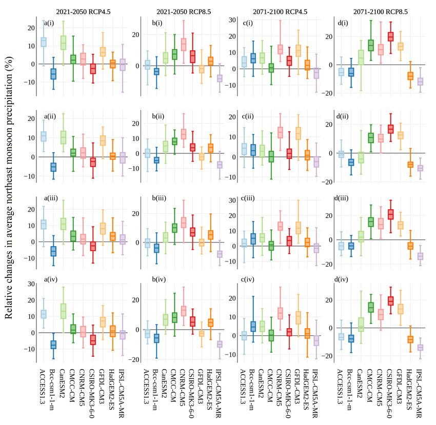
Water 2019, 11, 2300                                                                              2 of 22

several hundreds of kilometers) is too coarse to be directly used in regional or local climate change
studies, downscaling approaches have to be developed to bridge the scale discrepancy between
GCM grid-scale and the resolution required by regional or local studies. Dynamical downscaling
(DD) and statistical downscaling (SD) are two types of approaches frequently used to downscale
GCM outputs from GCM grid-scale to regional and local scales. The DD approach nests a regional
climate model (RCM) (with spatial resolution in the order of tens of kilometers) into the parent
GCMs, using GCM outputs as boundary conditions [1–3]. Although the DD approach is able to
generate finer-resolution climate data, the scale discrepancy remains between the RCM grid-scale
and the site-specific scale required by local studies. Besides, the RCM outputs are also subject to
biases inherited from the parent GCMs as well as from their own model deficiencies [4]. In contrast
to the DD approach, the SD approach is computationally easier because no physical representation
or parameterization is involved, and only statistical links are established between the large-scale
predictors and local-scale predictands. The SD approaches are generally categorized into three
groups [4]: perfect prognosis (PP; also referred to as “perfect prog”), model output statistics (MOS)
and stochastic weather generator (WG). For detailed reviews of these approaches, references are made
to the works of Wilby and Wigley [5], Xu [6], Fowler et al. [7], Maraun et al. [4], and Schoof [8].
      In the broad family of statistical downscaling, the WG approach has received widespread
attention in recent decades due to its adaptability and flexibility in climate change studies. Weather
generators are stochastic models which are able to generate ensembles of weather sequences with
similar statistical properties as the observed one. Downscaling using WGs is done through perturbing
the WG parameters according to the projected changes from climate models. This approach has been
applied in downscaling both GCM and RCM outputs. For instance, Fatichi et al. [9] used an hourly
weather generator to downscale the outputs from eight GCMs to the location of Tucson (AZ) for
both the present and future period. Similarly, based on the change factor method, Kilsby et al. [10]
developed a daily weather generator to generate site-specific meteorological series for the UK Climate
Impacts Programme (UKCIP02) scenarios derived from the HadRM3H integrations.
      Conventional downscaling approaches based on WGs are often single-site based, thus can
only provide climate change scenarios at single locations or independently at multiple locations.
The negligence of inter-site dependence in the downscaled meteorological fields could lead to
misrepresentation of the extremes of hydrological response variables in subsequent hydrological
impact studies. In addition, the inter-variable relationship between meteorological variables (e.g.,
the relationship between precipitation and temperature) should be respected to maintain the physical
coherence in the downscaling procedure. As shown by Chen et al. [11], the ignorance of inter-variable
correlation in the bias-correction of GCM outputs could lead to biases not only in the individual
distributions, but also in their correlations, which in turn results in biased hydrological simulations.
      All these issues necessitate the development of multi-site multivariate WGs (MMWGs)—with
reliable representation of the inter-site and inter-variable dependence structures—for downscaling
large-scale climate model outputs (please refer to Li and Babovic [12] for a detailed review of MMWGs).
To fill such a research gap, efforts have been devoted to develop MMWGs with application to multi-site
multivariate downscaling. Steinschneider and Brown [13] proposed a semi-parametric MMWG which
integrates several components including a wavelet decomposition coupled to an autoregressive model
to take account of low-frequency climate oscillations, a Markov chain and k-nearest-neighbor (KNN)
resampling scheme to model the inter-site and inter-variable dependencies, and a quantile mapping
procedure to allow for long-term distributional shifts resulting from prescribed climate changes.
The proposed approach was shown to be effective in simulating spatially distributed, multivariate
weather series for climate risk assessment. Chen et al. [14] proposed a hybrid approach which
couples a spatial downscaling method and a temporal downscaling approach based on a MMWG
(MulGETS, Chen et al. [15]). This approach was used to downscale the monthly precipitation from
the National Centers for Environment Prediction (NCEP) data to daily precipitation data at ten
stations over Hanjiang river basin in south-central China. As shown by Chen et al. [14], the proposed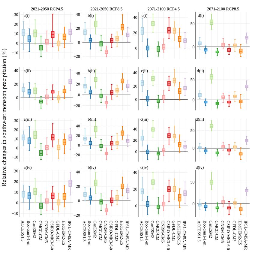
Water 2019, 11, 2300 3 of 22
approach was able to reconstruct the distributional statistics as well as the spatial dependence
in the downscaled precipitation field for the validation period. However, given that the spatial
correlation in MulGETS is taken into account by driving the single-site WG by temporally-independent
but spatially-correlated random numbers based on the Iman shuffling method [16], the temporal
persistence as well as inter-annual variability would not be maintained in the downscaled GCM
outputs [12]. Likewise, Li et al. [17] presented a two-stage spatiotemporal downscaling approach,
where, in the first step, spatial and temporal downscaling procedures were conducted based,
respectively, on quantile mapping and a single-site Richardson-type WG, and then the inter-site
and inter-variable dependencies in the downscaled GCM outputs were reconstructed using the Iman
shuffling method as a post-processing technique in the second step. This approach is an extended
application of the two-stage MMWG of Li [18]. However, as shown by Li and Babovic [12], the Iman
shuffling method is incapable of reproducing the temporal structure in the post-processed series.
To address this issue, Li and Babovic [12] proposed a two-stage MMWG based on Empirical Copula
(EC) approach (MMWG-EC), in which the meteorological series are first simulated from a single-site
multivariate WG, and then the inter-site and inter-variable dependencies, temporal persistence,
and inter-annual variability are reconstructed using the EC approach. The proposed method was
shown to outperform the one based on Iman shuffling, especially for restoring the temporal structures
in the simulated meteorological series. To extend the proposed MMEG-EC approach to a multi-site
multivariate climate downscaling context, Li and Babovic [19] proposed an integrated framework
combining quantile mapping, stochastic WG, and the EC approaches for multi-site multivariate
downscaling of global climate model outputs. The proposed method was applied to the Daqing River
basin in north China, to downscale the monthly, grid-based GCM data to daily, station-based data at
eleven stations over the catchment. As shown by Li and Babovic [19], the proposed approach performs
reasonably well in restoring the marginally distributional statistics, temporal persistence, inter-site and
inter-variable dependencies, and some extent of the inter-annual variability for the validation period.
Precipitation and temperature changes are complex in tropical urban regions such as Singapore,
because the meteorological processes are influenced by the combined effects of natural climate
variability, anthropogenic climate change and the local processes [20]. Precipitation in Singapore
is often influenced by small-scale convective storms; thus, to model the change in precipitation
extremes in future, downscaling approaches should be conducted at local scale, and at the same
time the multi-site correlation should be preserved to reflect the actual spatial consistency and
variability. Besides, as found by Li et al. [20], there are significant correlations between precipitation
extremes and local temperature, which necessitates the use of a multi-variate downscaling approach in
order to preserve the precipitation–temperature relationship in the downscaling procedure. Finally,
to understand the spatial variability of the projected changes in precipitation and temperature in
the Singapore region, a multi-site multivariate downscaling approach is desired. All these factors
motivated this study.
Therefore, the primary objective of this study was to examine the projected changes in daily
precipitation, maximum and minimum temperatures in Singapore, based on the newly developed
multi-site multivariate downscaling approach of Li and Babovic [19]. To better characterize the
uncertainty due to different schemes of GCMs, outputs from nine Earth System Models (ESMs) were
downscaled. The projected changes in daily precipitation, maximum and minimum temperatures were
examined, focusing on the changes in annual and seasonal means of precipitation and temperature.
In addition, changes in average wet and dry spell lengths were also investigated.
2. Study Area and Observational Data
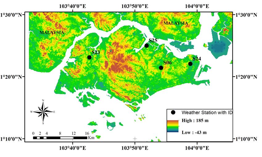
Singapore, a highly urbanized city-state with an area of around 719 km2 , is located off the
southern tip of Malay Peninsula, separated from Peninsular Malaysia by Johor Straits to the north
and from Indonesia’s Riau Islands by the Singapore Strait to the south (see Figure 1). Singapore is
situated one degree (137 km) north of the equator, and has a typically tropical climate with abundant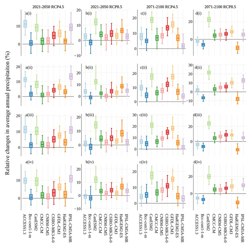
Water 2019, 11, 2300                                                                                     4 of 22

rainfall, high and uniform temperatures, and high humidity all year round. The long-term (1980–2010)
mean annual precipitation is 2430 mm, with the average of 51% rainy days [21]. The highest daily
precipitation depth in the historical record is 512.4 mm (recorded in December 1978) [22]. Annual
mean temperature is around 26–27.5 ◦ C [23]. Singapore’s climate is characterized by two major
monsoon seasons, i.e., the northeast monsoon season (from the end of October to early March) and
the southwest monsoon (from June to September) [24]. Spatial variability of precipitation field is
also observed for Singapore [25,26]. The long-term (1985–2014) daily precipitation, and maximum
and minimum temperatures at four weather stations in Singapore (see Figure 1) were sourced
from Meteorological Services Singapore (see http://www.weather.gov.sg/climate-historical-daily/).
These three meteorological variables are often used as inputs to hydrological models; therefore,
the investigation of their changes has great implication for further hydrological impact study.

      Figure 1. Location of weather stations in Singapore (elevation derived from the 90 m SRTM DEM [27]).

3. Methodology

3.1. Selection of Large-Scale Climate Models
     Large-scale monthly model simulation and projection data from nine Earth System Models
(ESMs, also referred to as GCMs) under historical forcing and two representative concentration
pathways (RCPs) scenarios were used for downscaling. The two RCPs used are RCP4.5 and RCP8.5,
which represent two emission scenarios under which the radiative forcing value in the year 2100
is approximately 4.5 and 8.5 W/m2 , respectively, higher than the preindustrial value. The nine
ESMs were used by Marzin et al. [28] for Singapore’s second national climate change study and are
deemed to perform well in simulating the climate characteristics in Southeast Asia. It is necessary to
emphasize here that, in the proposed downscaling approach, only the monthly GCM data are required.
This renders the proposed methodologies more reliable given that monthly GCM outputs are more
credible and readily available than those at daily scale [29]. The large-scale monthly GCM data were
obtained from phase 5 of the Coupled Model Intercomparison Project (CMIP5, Taylor et al. [30]) model
archive (http://cmip-pcmdi.llnl.gov/cmip5/). Since most of the GCM historical simulations end
in 2005, to align with the historically observed record, historical simulation data for all the GCMs
were extended to 2014 using their respective RCP4.5 simulations [31]. For the multi-site multivariate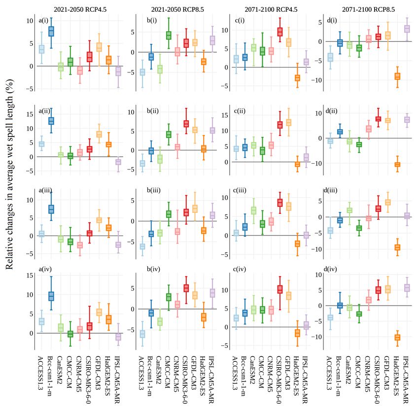
Water 2019, 11, 2300                                                                                      5 of 22

downscaling, the historical period 1985–2014 was considered as the control period, during which
the calibration of the methodologies was performed, and the periods of 2021–2050 and 2071–2100
were used as the mid- and end-century projection periods, during which the multi-site multivariate
downscaling was conducted. The detailed information about the selected GCMs are given in Table 1.

            Table 1. Large-scale climate models used for future climate change scenario construction.

    Earth System                                               Resolution
                                Institution                                           Emission Scenarios
      Models                                            (Latitude × Longitude)
                       Commonwealth Scientific and
                       Industrial Research
     ACCESS1.3         Organisation, Australia               1.25◦ × 1.875◦         historical, RCP4.5, RCP8.5
                       (CSIRO), and Bureau of
                       Meteorology, Australia (BOM)
    Bcc-csm1-1-m       Beijing Climate Center              2.7906◦ × 2.8125◦        historical, RCP4.5, RCP8.5
                       Canadian Centre for Climate
      CanESM2                                              2.7906◦ × 2.8125◦        historical, RCP4.5, RCP8.5
                       Modelling and Analysis
                       Centro Euro-Mediterraneo per
     CMCC-CM                                                 0.7484◦ × 0.75◦        historical, RCP4.5, RCP8.5
                       I Cambiamenti Climatici
                       Centre National
                       de Recherches
                       Meteorologiques/Centre
    CNRM-CM5                                               1.4008◦ × 1.40625◦       historical, RCP4.5, RCP8.5
                       Europeen de Recherche et
                       Formation Avancees en
                       Calcul Scientifique
                       Commonwealth Scientific and
                       Industrial Research
  CSIRO-MK3-6-0        Organisation in collaboration        1.8653◦ × 1.875◦        historical, RCP4.5, RCP8.5
                       with the Queensland Climate
                       Change Centre of Excellence
                       Geophysical Fluid
     GFDL-CM3                                                  2◦ × 2.5◦            historical, RCP4.5, RCP8.5
                       Dynamics Laboratory
   HadGEM2-ES          Met Office Hadley Centre              1.25◦ × 1.875◦         historical, RCP4.5, RCP8.5
  IPSL-CM5A-MR         Institut Pierre-Simon Laplace         1.2676◦   ×   2.5◦     historical, RCP4.5, RCP8.5

3.2. The Multi-Site Multivariate Downscaling Approach
     The multi-site multivariate downscaling approach of Li and Babovic [19] consists of three steps.
The first step is spatial downscaling, in which quantile mapping method is used to downscale monthly
data from GCM grid-scale to site-specific scale. For the second step, temporal downscaling is conducted,
in which the spatially-downscaled site-specific monthly data are further downscaled to daily data,
by adjusting the parameters of a Richardson-type WG. In the last step, the EC approach is utilized to
restore the observed inter-site and inter-variable dependencies as well as the temporal structures in
the downscaled GCM outputs.

3.2.1. Spatial Downscaling
      Before applying spatial downscaling, an inverse distance weighting method was used to
interpolate the original large-scale GCM values at four nearest neighboring grid points to the grid box
centered at the target station. The interpolation based on four nearest neighboring grid points is to
avoid the risk of non-representative GCM data for point-scale climate change study [32,33].
      A quantile mapping method, proposed by Zhang [34], was utilized to downscale the monthly
GCM data from grid-scale to site-specific scale. This method has been applied in several studies
(e.g., [14,17,32,35,36]), and is deemed to be effective in reproducing the cumulative distribution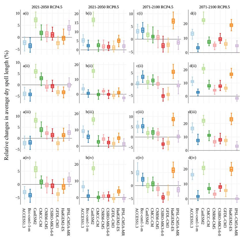
Water 2019, 11, 2300                                                                               6 of 22

functions (CDFs) of local observations in the downscaled data. First, the first- and third-order
polynomials were fitted between the sorted (in ascending order) monthly data (monthly sum for
precipitation and monthly means for maximum and minimum temperatures) of the observations
and those of the GCMs for each calendar month (e.g., for January, the monthly data refer to data
corresponding to January 1985, January 1986,. . . , January 2014) of the control period. Then, the fitted
polynomials were used as transfer functions to downscale the GCM monthly data for the projection
periods. More specifically, the third-order polynomials were used to downscale the monthly GCM
values that are within the range in which the third-order polynomials were fitted, given their better
goodness-of-fit than the first-order ones. For the out-of-range values, conservative approximations
were generated based on the fitted first-order polynomials [14,34]. Mean and variance of the spatially
downscaled GCM monthly data of the projection periods were calculated for each variable, each
calendar month, and each station, which were used subsequently in the temporal downscaling scheme.

3.2.2. Temporal Downscaling
     A Richardson-type WG [37] was used for temporal downscaling. Daily precipitation
was simulated by a chain-dependent process, in which precipitation occurrence was modeled
by a first-order two-stage Markov chain, and precipitation amount on a wet day (daily
precipitation ≥ 0.1 mm) was generated by a two-parameter Gamma distribution. For the modeling of
daily maximum and minimum temperatures (Tmax and Tmin), the normal distribution of [17] was
preferred, being it simpler than the first-order autoregressive model of Richardson [37]. Given the
stochastic nature of the WG, an ensemble of 100 independent simulations was generated, each with a
length equal to that of the projection periods. To downscale the spatially-downscaled GCM monthly
data to daily data for the projection periods, parameters in the precipitation, maximum and minimum
temperature models of the WG needed to be adjusted accordingly.
     For downscaling of the precipitation, parameters needed to be determined for both the
precipitation occurrence model (parameters being two transition probabilities) and precipitation
amount model (parameters related to mean daily precipitation per wet day and daily precipitation
variance for the wet days) for the projection periods. For precipitation occurrence, transition
probabilities of the projection periods were determined based on a four-point linear regression
method (regression between related precipitation occurrence model parameters and mean monthly
precipitation for each calendar month and each station) calibrated using historical data [14,38,39].
For precipitation amount, the mean daily precipitation per wet day for the projection periods was
calculated using the analytical approximation method of Wilks [40] based on the spatially-downscaled
GCM mean monthly precipitation of the projection periods [19]. The daily precipitation variance was
computed based on the proportional method of Zhang et al. [41], by multiplying the observed daily
precipitation variance of the control period by the calculated variance ratios. The monthly variance
ratios were calculated between the spatially-downscaled GCM monthly precipitation of the projection
periods and the local monthly data of the control period for each month and each station.
     Downscaling of GCM grid-scale monthly maximum and minimum temperatures for the projection
periods involved perturbing the mean and variance of daily maximum and minimum temperatures for
each calendar month and each station. The spatially-downscaled GCM mean monthly maximum and
minimum temperatures of the projection periods were directly used as the adjusted mean daily
values [34]. Similar to precipitation, adjusted daily temperature variances were determined by
multiplying the observed daily temperature variances of the control period by the calculated monthly
variance ratios (ratios between the spatially-downscaled GCM monthly temperatures and the observed
local monthly temperatures of the control period).

3.2.3. The Empirical Copula Approach
     The spatially and temporally downscaled GCM data (hereafter referred to as the “GCM-STD”
data) were post-processed using the Empirical Copula (EC) approach to restore the observed temporal,
Water 2019, 11, 2300 7 of 22
inter-site, and inter-variable dependencies. Empirical copulas [42–45]—with dependence structure
defined by independent rank transformations of the samples in each of the dimensions of the
multivariate data space–provide an ideal avenue for data post-processing. According to the definition
of EC, if two multivariate data samples have identical rank structures, their empirical copula templates
as well as all the information (including the temporal ordering characteristics and the inter-variable
dependence structures) thereof encoded, are the same. That said, if we re-order a multivariate
data sample according to the ranks in each dimension of some “reference” sample, the temporal
ordering characteristics and multivariate relationships encoded in such “reference” sample are
reconstructed. Moreover, being a post-processed technique that only manipulates the temporal
ordering of the data points, all the marginally distributional attributes of the “to-be-processed” data
points remain untouched.
A rank ordering technique adapted from the Schaake Shuffle method of Clark et al. [46] was
used to post-process the “GCM-STD” data. The observed data of the control period were directly
used as the “reference” to build the EC template and subsequently used to re-order the“GCM-STD”
data, such that the observed temporal structures and the inter-site and inter-variable dependencies
were reconstructed in the post-processed GCM-STD data (hereafter referred to as the “GCM-STD-EC”
data) for the projection periods. To account for the effect of seasonality, the rank ordering method was
performed separately for each of the combinations (3 variables × 4 stations in this study) for each
calendar month (the number of data points for each month = number of years × number of days for
that month; e.g., 30 × 31 = 930 for January in this study). For illustrative examples of applying the
adapted Schaake Shuffle method, references are made to the works of Vrac and Friederichs [47] and Li
and Babovic [12] in the contexts of multivariate, multi-site bias correction and multivariate, multi-site
WGs, respectively.
The direct use of the observed data of the control period to build the EC template for the projection
periods implicitly assumes the stationarity of EC—namely, the temporal, inter-site, and inter-variable
dependencies remain constant, even in a non-stationary climate condition. In the climate downscaling
community, the inter-variable and inter-site dependence structures (especially for the inter-site
dependence) are often assumed to be stationary [17] or are treated as physical constraints [48] in
a multi-site multivariate downscaling or bias-correction contexts. For the temporal dependence,
the stationarity assumption might seem to be too strict, as temporal variabilities (from day-to-day
variability to inter-annual variability) might change from the historical period to a future period.
To explore the stationarity assumption of EC based on observational data, Li and Babovic [19]
compared three forms of dependence metrics including Lag-1 autocorrelation, inter-site Spearman
correlation, and inter-variable Spearman correlation (which are manifestations of the ranks structures,
or the EC template, of the data) between climate periods (the first-half 30-year calibration period
and the latter-half 30-year validation period during 1957–2016) with different climatology for the
Daqing River basin in north China. As shown, generally, these three forms of dependency metrics
remain constant, with slight differences in Lag-1 autocorrelation and inter-variable correlation for
some variables and variables pairs between the two periods. Moreover, the stationarity of these three
dependence metrics in a non-stationary climate condition has also been found in the Upper Thames
River basin in Canada [12]. Therefore, in the present study, we held the stationarity assumption of EC
in the multi-site multivariate downscaling approach, given its merits in reproducing the multi-site,
multivariate correlations, temporal persistence, and even some extent of the inter-annual variability in
the downscaled GCM outputs [19].
4. Results and Discussion
4.1. Assessment of Inter-Site, Inter-Variable, and Temporal Dependence Reconstruction
The performance of the EC approach for reconstructing the observed inter-site Spearman rank
correlation in the spatially-temporally downscaled meteorological field of ACCESS1.3 model underWater 2019, 11, 2300 8 of 22
RCP8.5 scenario over the period of 2071–2100 is evaluated in Figure 2. Similar performances were
found for the remaining GCMs across the emission scenarios and projection periods; however, due to
space limit, they are not presented here. For comparison, the results correspond to spatially-temporally
downscaled outputs without applying the EC approach are also presented. The median values of
inter-station correlations were taken over 100 different simulations and are compared against the
observed ones of the control period. As shown, the spatially-temporally downscaled ACCESS1.3
data without adopting the EC post-processing technique (ACCESS1.3-STD) are not able to restore
the observed inter-station correlations for all the meteorological variables. This is because, in the
ACCESS1.3-STD data, the meteorological variables are downscaled based on a single-site spatial
and temporal downscaling procedure, where no spatial links are introduced. In contrast, observed
inter-station correlations are well reproduced in the spatially-temporally downscaled ACCESS1.3 data
post-processed by the EC approach (ACCESS1.3-STD-EC) for precipitation occurrence, precipitation
amount, and maximum and minimum temperatures at both daily and monthly timescales (daily
precipitation occurrence and amount are summed up to monthly timescale, while daily maximum
and minimum temperatures are averaged to monthly timescale). This is expected since the rank
dependence structures of the observations are exactly honored in the ACCESS1.3-STD-EC data; thus,
the inter-station correlations are preserved.
Figure 2. Inter-site Spearman rank correlations for precipitation occurrence, precipitation amount,
maximum temperature, and minimum temperature for all possible station pairs and for all months
for observations and spatially-temporally downscaled ACCESS1.3 data under RCP8.5 scenario over
the period of 2071–2100. The four columns represent precipitation occurrence, precipitation amount,
maximum temperature, and minimum temperature, respectively. The two rows denote the results
for daily and monthly timescale, respectively. Median values across the 100 different simulations are
shown against the observed values.
Figure 3 presents the Lag-1 serial autocorrelations (calculated as the Pearson correlation
coefficients) for daily precipitation, maximum and minimum temperatures and the inter-variable cross
correlations (computed as the Spearman rank correlation coefficients) for each pair of variables across
the stations and months for both observations and the spatially-temporally downscaled ACCESS1.3
data under RCP8.5 scenario over the period of 2071–2100. Similar results are found for other GCMs
across the emission scenarios and projection periods, and are not presented here due to space limit.
As seen, the ACCESS1.3-STD data fail to represent the observed Lag-1 serial autocorrelations and
inter-variable correlations. This is because the WG used in this study is not capable of representing the
temporal persistence as well as the inter-variable relationships in the simulations. More specifically,Water 2019, 11, 2300 9 of 22
all the variables are modeled independently, and no autoregressive models are introduced to reflect the
short-term persistence behavior. In comparison, the EC approach—by inheriting the rank structures
from observation—successfully rebuilds the Lag-1 autocorrelation for daily precipitation, maximum
and minimum temperatures, and the inter-variable correlations for all the variable pairs.
Figure 3. Lag-1 serial autocorrelations for daily: (a) precipitation; (b) maximum temperature; and (c)
minimum temperature, as well as cross correlations (Spearman rank correlation) for: (d) precipitation
vs. maximum temperature; (e) precipitation vs. minimum temperature; and (f) maximum temperature
vs. minimum temperature, for all stations and months for observations and spatially-temporally
downscaled ACCESS1.3 data under RCP8.5 scenario over the period of 2071–2100. Median values
across the 100 different simulations are shown against the observed values.
4.2. Projected Climate Change
The proposed multi-site multivariate downscaling approach was applied to downscale
precipitation, maximum and minimum temperatures from nine GCMs from grid-based, monthly
scale to site-specific, daily scale at four weather stations in Singapore for the periods of 2021–2050
and 2071–2100 under RCP4.5 and RCP8.5 scenarios. The projected changes in annual and seasonal
precipitation, annual average temperature, and wet and dry spell characteristics were examined. Box
and whisker plots are utilized to summarize the results from 100 independent simulations, and the
range of the box and whisker plot represents the stochastic variability of the downscaling approach.
Noticing that, for each GCM, the downscaling result is ensemble-based, we focus on the sign of the
median (positive or negative) and the range of the change values, which reflect, respectively, whether
the change is more likely to be positive or negative, and the spread of the change. The statistical
significance of the change for each realization of the downscaling in the ensemble is not considered,
given that it would be complicated to draw a conclusion about the projected changes based on both
the statistical significance and the spread of the changes.Water 2019, 11, 2300 10 of 22
4.2.1. Changes in Annual/Seasonal Precipitation and Temperature
Figure 4 presents the relative changes in average annual precipitation projected by downscaled
precipitation outputs from nine GCMs under both RCP4.5 and RCP8.5 scenarios over the mid-century
(2021–2050) and end-century (2071–2100) periods relative to observed values during 1985–2014 across
the weather stations in Singapore. It should be emphasized here that the EC-component of the
multi-site multivariate statistical downscaling method does not play any role for annual or seasonal
means of precipitation and temperature, since it only operates on the temporal ordering of the
downscaled data. As can be seen, there is no general agreement with projections of change among
the GCMs. Both positive and negative changes in annual precipitation could happen in the future,
and the magnitude of the changes depend on the selected GCM, emission scenario, projection period,
and station of interest. Although the projected changes differ between different periods and scenarios,
the major uncertainty comes from the GCMs. Note that, for most of the GCMs, the projected median
change values are positive (more than half of the 100 realizations project positive changes) for both RCP
scenarios and projection periods, suggesting that the increase of annual precipitation is more likely.
This is consistent with the observed changes found by Beck et al. [25], Li et al. [26], and Li et al. [20],
showing that annual precipitation as well as annual wet-day precipitation totals have increased
significantly over the historical period. In addition, although the distances between these stations are
relatively small, the projected changes are different across the stations. For instance, for the 2071–2100
period under RCP8.5 scenario, changes of mean annual precipitations are projected to vary between
−15.9% and 30.8%, between −13.4% and 29.0%, between −16.6% and 33.7%, and between −16.9%
and 31.7%, respectively, for stations S06, S23, S24 and S25 across the GCMs. These projected ranges
widen further if the changes are assembled across the stations and GCMs. Changes of mean annual
precipitations in Singapore are projected to range between −5.4% and 20.6% and between −9.5%
and 25.9% over the mid-century period under RCP4.5 and RCP8.5 scenarios, respectively, across the
stations. For the end-century period, mean annual precipitation could change by from −4.3% to 28.9%
and from −16.9% to 33.7%, respectively, under RCP4.5 and RCP8.5 scenarios. Note that the range
of the projected ranges are assembled rather than averaged across the weather stations, hence they
represent the whole ranges of the projected changes over different weather stations in Singapore.
Figures 5 and 6 present, respectively, the relative changes in average northeast monsoon
and southwest monsoon precipitations. Similar to annual precipitation, the projected changes
in these two monsoon seasonal precipitation vary among the GCMs. Overall, average northeast
monsoon precipitation is projected to change by from −16.0% to 27.9% and from −19.5% to 29.2%
over the 2021–2500 period under RCP4.5 and RCP8.5 scenarios, respectively, across the stations.
For the 2071–2100 period, the projected changes in average northeast monsoon precipitation range
between −14.3% and 30.0% and between −22.1% and 32.5% under the RCP4.5 and RCP8.5 scenarios,
respectively. In comparison, the spreads of the projected changes in average southwest monsoon
precipitation under RCP4.5 and RCP8.5 scenarios, respectively, are between −15.4% and 41.8% and
between −29.7% and 50.9% over the 2021–2500 period, and between −13.9% and 54.8% and between
−31.5% and 77.8% over the 2071–2100 period.
For temperature, Figures 7 and 8 show, respectively, the changes in mean annual average daily
maximum and minimum temperatures projected by the GCMs under both RCP4.5 and RCP8.5
scenarios for the periods of 2021–2050 and 2071–2100 relative to observed values of 1985–2014.
Unlike precipitation, all the GCMs agree with the increases of average daily maximum and minimum
temperatures for both projection periods and for both emission scenarios. The changes in average
daily maximum and minimum temperatures could be felt differently at different stations. For instance,
for the end-century period under the RCP8.5 scenario, average daily minimum temperature is projected
to increase by 1.4–3.2 ◦ C and 3.1–6.5 ◦ C across the GCMs, respectively, for stations S23 and S06. Across
the stations, average daily maximum temperature are projected to increase by 0.6–1.6 ◦ C and 0.6–1.7 ◦ C
for the period of 2021–2050 under RCP4.5 and RCP8.5 scenarios, respectively. For average daily
minimum temperature over the period of 2021–2050, the projected increases are 0.4–1.8 ◦ C andWater 2019, 11, 2300 11 of 22
0.4–2.0 ◦ C, respectively, under RCP4.5 and RCP8.5 scenarios. The increases become even greater into
the future, with a projected increase of 0.9–3.0 ◦ C (under RCP4.5) and 2.0–5.7 ◦ C (under RCP8.5) for
average daily maximum temperature, and 0.6–3.6 ◦ C (under RCP4.5) and 1.4–6.5 ◦ C (under RCP8.5)
for average daily minimum temperature over the period of 2071–2100.
Figure 4. Relative changes (%) in long-term average annual precipitation from downscaled GCM
data for: (a) 2021–2050 period under RCP4.5 scenario; (b) 2021–2050 period under RCP8.5 scenario;
(c) 2071–2100 period under RCP4.5 scenario; and (d) 2071–2100 period under RCP8.5 scenario relative
to observed values during 1985–2014. Rows (i–iv) denote results for stations S06, S23, S24, and S25,
respectively. The bottom, middle, and top of the box denote the first, second, and third quartiles,
respectively. The lower and upper ends of the whiskers represent the minimum and maximum
values, respectively.Water 2019, 11, 2300 12 of 22
Figure 5. Relative changes (%) in long-term average northeast monsoon precipitation from downscaled
GCM data for: (a) 2021–2050 period under RCP4.5 scenario; (b) 2021–2050 period under RCP8.5
scenario; (c) 2071–2100 period under RCP4.5 scenario; and (d) 2071–2100 period under RCP8.5 scenario
relative to observed values during 1985–2014. Rows (i–iv) denote results for stations S06, S23, S24,
and S25, respectively. The bottom, middle, and top of the box denote the first, second, and third
quartiles, respectively. The lower and upper ends of the whiskers represent the minimum and
maximum values, respectively.Water 2019, 11, 2300 13 of 22
Figure 6. Relative changes (%) in long-term average southwest monsoon precipitation from downscaled
GCM data for: (a) 2021–2050 period under RCP4.5 scenario; (b) 2021–2050 period under RCP8.5
scenario; (c) 2071–2100 period under RCP4.5 scenario; and (d) 2071–2100 period under RCP8.5 scenario
relative to observed values during 1985–2014. Rows (i–iv) denote results for stations S06, S23, S24,
and S25, respectively. The bottom, middle, and top of the box denote the first, second, and third
quartiles, respectively. The lower and upper ends of the whiskers represent the minimum and
maximum values, respectively.Water 2019, 11, 2300 14 of 22
Figure 7. Delta changes in long-term average annual mean daily maximum temperature from
downscaled GCM data for: (a) 2021–2050 period under RCP4.5 scenario; (b) 2021–2050 period under
RCP8.5 scenario; (c) 2071–2100 period under RCP4.5 scenario; and (d) 2071–2100 period under RCP8.5
scenario relative to observed values during 1985–2014. Rows (i–iv) denote results for stations S06,
S23, S24, and S25, respectively. The bottom, middle, and top of the box denote the first, second,
and third quartiles, respectively. The lower and upper ends of the whiskers represent the minimum
and maximum values, respectively.
It might be interesting to compare the change signal produced by the original GCM projections
and by the downscaled data. Figure 9 presents the changes in mean monthly precipitation (% change)
and mean monthly maximum and minimum temperatures (delta change) for the 2071–2100 period
under RCP8.5 scenario relative to the observed values during the baseline period (1985–2014) for both
the original GCM data and the downscaled data at station S24. As seen, for precipitation and maximum
and minimum temperatures, the spatially downscaled data produce different change signals (in terms
of both magnitude and direction of change) compared with the original GCM data. For example,
we see less changes in average monthly precipitation in downscaled data compared with the original
GCMs. For temperature, the downscaled data show consistent increase of average monthly maximum
and minimum temperatures. In comparison, some GCMs show decrease of mean monthly maximum
temperature for January, February, March, and April. The difference in change signals between originalWater 2019, 11, 2300 15 of 22
GCM data and the downscaled ones indicate that climate change information might be different at
different spatial scales. This has important implications for regional or local climate change studies.
Figure 8. Delta changes in long-term average annual mean daily minimum temperature from
downscaled GCM data for: (a) 2021–2050 period under RCP4.5 scenario; (b) 2021–2050 period under
RCP8.5 scenario; (c) 2071–2100 period under RCP4.5 scenario; and (d) 2071–2100 period under RCP8.5
scenario relative to observed values during 1985–2014. Rows (i–iv) denote results for stations S06,
S23, S24, and S25, respectively. The bottom, middle, and top of the box denote the first, second,
and third quartiles, respectively. The lower and upper ends of the whiskers represent the minimum
and maximum values, respectively.Water 2019, 11, 2300 16 of 22
Figure 9. Relative Changes in mean monthly precipitation (first row,in %), mean monthly maximum
temperature (second row; delta change), mean monthly minimum temperature (third row; delta change)
for the 2071–2100 period under RCP8.5 scenario relative to the observed values during 1985–2014 at
station S24. Left column denotes the original GCM values, right column represents the spatially and
temporally downscaled GCM values.
In summary, the climate change signal over the Singapore region is more consistent for
temperature than for precipitation. The mean annual average daily maximum and minimum
temperatures are projected to increase over both the mid-century and end-century periods under both
RCP4.5 and RCP8.5 emission scenarios. For precipitation, the projected changes vary across GCMs,
RCPs, and projection periods at both annual and seasonal timescales. Similar results were found
by Marzin et al. [28] based on a dynamical downscaling approach. As shown by Marzin et al. [28],
there was a consensus on increase of annual average daily maximum and minimum temperatures,
with increase becoming greater from RCP4.5 scenario to RCP8.5 scenario, and from mid-century
period to end-century period; however, for precipitation, as shown by Marzin et al. [28], disagreement
was observed among the GCMs, and both positive and negative changes in annual and seasonal
precipitation could happen, which are independent of emission scenarios.
4.2.2. Changes in Average Wet and Dry Spell Lengths
The day-to-day variability of precipitation can be characterized by wet and dry spells. The change
in wet and dry spell characteristics has great impact on hydrology, agriculture, ecology and water
resources management. A wet (dry) spell is defined as the number of consecutive rainy (non-rainy)
days (a rainy day is defined as the day with daily precipitation ≥ 1 mm). A number of dry and wet
spell indices (e.g., see Li et al. [26] and Li et al. [49]) could be utilized to analyze the characteristics of
dry and wet spells; however, here, due to the space limit, we only focus on the changes in average
dry and wet spell length. Figures 10 and 11 present, respectively, the relative changes in average
dry and wet spell lengths with respect to the observed values during 1985–2014. It is necessary to
emphasize here that the EC-component of the multi-site multivariate downscaling approach plays
a significant role in building the wet and dry spell characteristics. As seen, most of the GCMs tend
to project positive median change values for average dry spell length over both the 2021–2050 and
2071–2100 periods under both emission scenarios. This indicates that average dry spell length is moreWater 2019, 11, 2300 17 of 22
likely to increase over the 2021–2050 and 2071–2100 periods under both RCP4.5 and RCP8.5 scenarios.
Compared with average dry spell length, less consensus is observed about the projected changes
in average wet spell length. Overall, average dry spell length is projected to change by −7.3–11.4%
and −4.7–21.4% over the 2021–2500 period under RCP4.5 and RCP8.5 scenarios, respectively. For the
period of 2071–2100, the spreads of the projected changes in average dry spell length are −7.5–11.7%
and −3.8–28.1% under RCP4.5 and RCP8.5 scenarios, respectively. For average wet spell length, the
ranges of the projected changes under RCP4.5 and RCP8.5 scenarios, respectively, are −5.6–17.1%
and −8.9–11.0% over the 2021–2050 period, and −5.4–17.2% and −13.4–11.9% over the 2071–2100
period. These projected changes have implications for adaptation planning and risk reduction in water
resources management in Singapore.
Figure 10. Relative changes (%) in average dry spell lengths from downscaled GCM data for:
(a) 2021–2050 period under RCP4.5 scenario; (b) 2021–2050 period under RCP8.5 scenario; (c) 2071–2100
period under RCP4.5 scenario; and (d) 2071–2100 period under RCP8.5 scenario relative to observed
values during 1985–2014. Rows (i–iv) denote results for stations S06, S23, S24, and S25, respectively.
The bottom, middle, and top of the box denote the first, second, and third quartiles, respectively.
The lower and upper ends of the whiskers represent the minimum and maximum values, respectively.Water 2019, 11, 2300 18 of 22
Figure 11. Relative changes (%) in average wet spell lengths from downscaled GCM data for:
(a) 2021–2050 period under RCP4.5 scenario; (b) 2021–2050 period under RCP8.5 scenario; (c) 2071–2100
period under RCP4.5 scenario; and (d) 2071–2100 period under RCP8.5 scenario relative to observed
values during 1985–2014. Rows (i–iv) denote results for stations S06, S23, S24, and S25, respectively.
The bottom, middle, and top of the box denote the first, second, and third quartiles, respectively.
The lower and upper ends of the whiskers represent the minimum and maximum values, respectively.
4.2.3. Uncertainty of the Projection Results
The projection results presented in this paper may be subject to a cascade of uncertainties resulting
from several factors. The first one is related to the choice of GCMs. In the present study, only nine
GCMs were used for downscaling, and, for each GCM, only the first realization (r1i1p1) was used.
As such, the full range of potential climate change as well as the impact of the initialization of
GCMs (e.g., the impact of the different atmospheric conditions used at the start of each experiment)
on the projection results might not be well represented. Second, we only used two representative
concentration pathways, i.e., the RCP4.5 and RCP8.5 scenarios, as the prescribed future emission
scenarios, which may not cover the entire set of possible greenhouse gas emission scenarios. Third,
all the large-scale GCM outputs were downscaled by using only one statistical downscaling method,
i.e., the multi-site, multivariate downscaling approach of Li and Babovic [19]; therefore, uncertainty
due to the choice of downscaling techniques can also be expected.Water 2019, 11, 2300 19 of 22
In this study, the uncertainties were linked to GCMs, RCP scenarios, and the stochastic variability
of the multi-site multivariate downscaling method. As the last one could be clearly represented by
the range of the boxes from the 100 realizations, we place our focus on the uncertainties resulted
from GCMs and RCPs. Figure 12 shows the relative changes (%) in average annual precipitation
versus the delta changes in average annual mean daily maximum temperature for different GCMs
and RCP scenarios for the 2071–2100 period at station S06. Since, for each GCM and RCP, there
are 100 realizations of projections, to put aside the uncertainty from the stochastic variability of the
downscaling method, the median values of the 100 realizations are shown. As seen, the uncertainties
related to the GCMs and RCPs are evident. For instance, six GCMs (in the vertical blue rectangle in
Figure 12) project similar increases of temperature but different changes in precipitation under RCP4.5
scenario. Similarly, four GCMs (in the horizontal red rectangle in Figure 12) project similar changes in
precipitation but different increases of temperature under RCP8.5 scenario. The projected directions
of change in precipitation differ even for different RCPs (for instance, the median change values for
ACCESS1.3, Bcc-csm1–1-m, and HadGEM2-ES under RCP 4.5 scenario differ in direction from RCP8.5
scenario; see Figure 4c(i),d(i) for details). Overall, the uncertainty ranges of RCP8.5 scenario is larger
than those of RCP4.5 scenario, for both precipitation and temperature.
Figure 12. Projected relative changes (%) in average annual precipitation and delta changes (◦ C) in
average annual mean daily maximum temperature for different GCMs and RCPs for the 2071–2100
period at station S06. The median value of the 100 realizations is shown for a given GCM and RCP.
With respect to the multi-site, multivariate downscaling approach itself, the assumptions involved
in the different stage of downscaling also have impacts on the projections results. For example, for the
quantile mapping approach used in the spatial downscaling, the regression relationship fitted between
the GCM grid-scale monthly data and the local station-specific ones are assumed to be stationary.
Based on such an assumption, Mullan et al. [36] demonstrated the capability of the quantile mapping
approach in reproducing the observed distributional statistics in a non-stationary climate condition.
However, it could also be expected that the regression weights fitted based on historical data would
change through time, leading to a deterioration of performance for quantile mapping over a future
period. Besides, the non-stationarity of the GCM biases could also affect the performance of quantile
mapping. Another important assumption made in the downscaling approach is the stationarity of EC
for post-processing the spatially-temporally downscaled GCM outputs. Whether this assumption is
valid under a non-stationary climate condition determines the performance of the proposed multi-site
multi-variate downscaling approach in representing the various forms of dependencies. One mayWater 2019, 11, 2300 20 of 22
argue that this assumption might be more valid during the mid-century period than during the
end-century period, given that climate condition is more likely to change in the distant future than
in the near future. However, this was not considered in the present study, since we assumed the
stationarity of EC throughout the future period.
5. Conclusions
A reliable estimate of the projected changes in precipitation and temperature has great significance
for subsequent impact modeling and adaption planning in the context of climate change. To generate
spatially-distributed and physically coherent climate projections at regional scale, multi-site and
multivariate downscaling approaches are often desired to reflect the inter-site and inter-variable
dependence structures in the downscaled meteorological field. In this study, mid-term and long-term
projections of precipitation and maximum and minimum temperatures at four weather stations of the
Singapore region were generated using a newly developed multi-site and multivariate downscaling
approach. This downscaling approach was evaluated fully by Li and Babovic [19].
The projections show that average maximum and minimum temperatures in Singapore would
increase in the future, while annual precipitation may increase or decrease, depending on the GCMs
and emission scenarios. The major uncertainty of precipitation projection comes from GCMs, which
implies that an ensemble of GCMs is needed for impact assessment in this region. The projected
changes in precipitation and temperature in Singapore may affect various aspects of the natural
environment, public heath, energy demand, and urban infrastructure. To cope with the projected
climate changes, appropriate adaption strategies should be formulated and they should be flexible to
incorporate future knowledge of climate change to safeguard the nation against the potential risks.
The multi-site multivariate downscaling method used in this study can: (1) provide a
distributed, physically coherent downscaled meteorological fields for subsequent impact modeling
in different fields; and (2) generate an ensemble of realizations of climate change scenarios for better
characterization of the uncertainty in the era of global warming. Future research should focus on
the coupling of this method with hydrological models, to analyze the climate change impact on
hydrological variabilities. Moreover, comparison studies with other downscaling approaches across
diverse climate and topographies would also be interesting.
Author Contributions: Conceptualization, X.L.; methodology, X.L. and K.Z.; formal analysis, X.L., K.Z., and V.B.;
investigation, X.L. and K.Z.; writing—original draft preparation, X.L.; writing—review and editing, X.L., K.Z.,
and V.B.; visualization, X.L.; funding acquisition, K.Z. and X.L.
Funding: This research was funded by National Natural Science Foundation of China grant number 51909061,
Natural Science Foundation of Jiangsu Province grant number BK20180022, Fundamental Research Funds for the
Central Universities grant number 2019B01614, and Six Talent Peaks Project in Jiangsu Province grant number
NY-004.
Conflicts of Interest: The authors declare no conflict of interest.
References
1. Giorgi, F.; Shields Brodeur, C.; Bates, G.T. Regional climate change scenarios over the United States produced
with a nested regional climate model. J. Clim. 1994, 7, 375–399. [CrossRef]
2. Fu, C.; Wang, S.; Xiong, Z.; Gutowski, W.J.; Lee, D.K.; McGregor, J.L.; Sato, Y.; Kato, H.; Kim, J.W.; Suh,
M.S. Regional climate model intercomparison project for Asia. Bull. Am. Meteorol. Soc. 2005, 86, 257–266.
[CrossRef]
3. Jeong, D.I.; Sushama, L.; Diro, G.T.; Khaliq, M.N.; Beltrami, H.; Caya, D. Projected changes to high
temperature events for Canada based on a regional climate model ensemble. Clim. Dyn. 2016, 46, 3163–3180.
[CrossRef]
4. Maraun, D.; Wetterhall, F.; Ireson, A.; Chandler, R.; Kendon, E.; Widmann, M.; Brienen, S.; Rust, H.; Sauter, T.;
Themeßl, M.; et al. Precipitation downscaling under climate change: Recent developments to bridge the gap
between dynamical models and the end user. Rev. Geophys. 2010, 48. [CrossRef]Water 2019, 11, 2300 21 of 22
5. Wilby, R.L.; Wigley, T. Downscaling general circulation model output: A review of methods and limitations.
Prog. Phys. Geogr. 1997, 21, 530–548. [CrossRef]
6. Xu, C.Y. From GCMs to river flow: A review of downscaling methods and hydrologic modelling approaches.
Prog. Phys. Geogr. 1999, 23, 229–249. [CrossRef]
7. Fowler, H.J.; Blenkinsop, S.; Tebaldi, C. Linking climate change modelling to impacts studies: Recent
advances in downscaling techniques for hydrological modelling. Int. J. Climatol. 2007, 27, 1547–1578.
[CrossRef]
8. Schoof, J.T. Statistical downscaling in climatology. Geogr. Compass 2013, 7, 249–265. [CrossRef]
9. Fatichi, S.; Ivanov, V.Y.; Caporali, E. Simulation of future climate scenarios with a weather generator.
Adv. Water Resour. 2011, 34, 448–467. [CrossRef]
10. Kilsby, C.; Jones, P.; Burton, A.; Ford, A.; Fowler, H.; Harpham, C.; James, P.; Smith, A.; Wilby, R. A daily
weather generator for use in climate change studies. Environ. Model. Softw. 2007, 22, 1705–1719. [CrossRef]
11. Chen, J.; Li, C.; Brissette, F.P.; Chen, H.; Wang, M.; Essou, G.R. Impacts of correcting the inter-variable
correlation of climate model outputs on hydrological modeling. J. Hydrol. 2018. [CrossRef]
12. Li, X.; Babovic, V. A new scheme for multivariate, multisite weather generator with inter-variable, inter-site
dependence and inter-annual variability based on empirical copula approach. Clim. Dyn. 2019, 52, 2247–2267.
[CrossRef]
13. Steinschneider, S.; Brown, C. A semiparametric multivariate, multisite weather generator with low-frequency
variability for use in climate risk assessments. Water Resour. Res. 2013, 49, 7205–7220. [CrossRef]
14. Chen, J.; Chen, H.; Guo, S. Multi-site precipitation downscaling using a stochastic weather generator.
Clim. Dyn. 2018, 50, 1975–1992. [CrossRef]
15. Chen, J.; Brissette, F.P.; Zhang, X.J. A multi-site stochastic weather generator for daily precipitation and
temperature. Trans. ASABE 2014, 57, 1375–1391.
16. Iman, R.L.; Conover, W.J. A distribution-free approach to inducing rank correlation among input variables.
Commun. Stat.-Simul. Comput. 1982, 11, 311–334. [CrossRef]
17. Li, Z.; Shi, X.; Li, J. Multisite and multivariate GCM downscaling using a distribution-free shuffle procedure
for correlation reconstruction. Clim. Res. 2017, 72, 141–151. [CrossRef]
18. Li, Z. A new framework for multi-site weather generator: A two-stage model combining a parametric
method with a distribution-free shuffle procedure. Clim. Dyn. 2014, 43, 657–669. [CrossRef]
19. Li, X.; Babovic, V. Multi-site multivariate downscaling of global climate model outputs: An integrated
framework combining quantile mapping, stochastic weather generator and empirical copula approaches.
Clim. Dyn. 2019, 52, 5775–5799. [CrossRef]
20. Li, X.; Wang, X.; Babovic, V. Analysis of variability and trends of precipitation extremes in Singapore during
1980–2013. Int. J. Climatol. 2018, 38, 125–141. [CrossRef]
21. Mandapaka, P.V.; Qin, X. Analysis and Characterization of Probability Distribution and Small-Scale Spatial
Variability of Rainfall in Singapore Using a Dense Gauge Network. J. Appl. Meteorol. Climatol. 2013,
52, 2781–2796. [CrossRef]
22. MSS. Annual Climatologicalreport; Technical Report; Meteorological Service Singapore: Singapore, 2014.
23. Chow, W.T.; Roth, M. Temporal dynamics of the urban heat island of Singapore. Int. J. Climatol. 2006,
26, 2243–2260. [CrossRef]
24. Fong, M.; Ng, L.K. The Weather and Climate of Singapore; Meteorological Service Singapore: Singapore, 2012.
25. Beck, F.; Bárdossy, A.; Seidel, J.; Müller, T.; Sanchis, E.F.; Hauser, A. Statistical analysis of sub-daily
precipitation extremes in Singapore. J. Hydrol. Reg. Stud. 2015, 3, 337–358. [CrossRef]
26. Li, X.; Meshgi, A.; Babovic, V. Spatio-temporal variation of wet and dry spell characteristics of tropical
precipitation in Singapore and its association with ENSO. Int. J. Climatol. 2016, 36, 4831–484. [CrossRef]
27. Jarvis, A.; Reuter, H.I.; Nelson, A.; Guevara, E. Hole-Filled SRTM for the Globe Version 4. 2008. Available
online: http://srtm.csi.cgiar.org (accessed on 11 August 2017).
28. Marzin, C.; Rahmat, R.; Bernie, D.; Bricheno, L.; Buonomo, E.; Calvert, D.; Cannaby, H.; Chan, S.;
Chattopadhyay, M.; Cheong, W.K.; et al. Singapore’s Second National Climate Change Study–Phase 1; Technical
Report; Met Office: Exeter, UK; Centre for Climate Researh Singapore and National Oceanography Centre:
Liverpool, UK; CSIRO, Australia and Newcastle University: Newcastle, UK, 2015.
29. Maurer, E.P.; Hidalgo, H.G. Utility of daily vs. monthly large-scale climate data: An intercomparison of two
statistical downscaling methods. Hydrol. Earth Syst. Sci. 2008, 12, 551–563. [CrossRef]You can also read