Tuna-AI: tuna biomass estimation with Machine Learning models trained on oceanography and echosounder FAD data
←
→
Page content transcription
If your browser does not render page correctly, please read the page content below
Tuna-AI: tuna biomass estimation with Machine
                                                   Learning models trained on oceanography and
                                                               echosounder FAD data

                                                                                             A Preprint
arXiv:2109.06732v3 [stat.ML] 29 Sep 2021

                                                              Daniel Precioso                              Manuel Navarro-Garcı́a
                                                       Department of Computer Science                Universidad Carlos III de Madrid, Spain
                                                        Higher School of Engineering                 Komorebi AI Technologies, Madrid, Spain
                                                         Universidad de Cádiz, Spain                    mannavar@est-econ.uc3m.es
                                                          daniel.precioso@uca.es

                                                   Kathryn Gavira-O’Neill             Alberto Torres-Barrán                   David Gordo
                                                           Satlink                    Komorebi AI Technologies             Komorebi AI Technologies
                                                        Madrid, Spain                      Madrid, Spain                        Madrid, Spain
                                                       kgo@satlink.es               alberto.torres@komorebi.ai            david.gordo@komorebi.ai

                                                             Vı́ctor Gallego-Alcalá                           David Gómez-Ullate∗
                                                            Komorebi AI Technologies                       Department of Computer Science
                                                                  Madrid, Spain                             Higher School of Engineering
                                                          victor.gallego@komorebi.ai                         Universidad de Cádiz, Spain
                                                                                                             david.gomezullate@uca.es

                                                                                              Abstract
                                                     Echo-sounder data registered by buoys attached to drifting FADs provide a very valuable
                                                     source of information on populations of tuna and their behaviour. This value increases when
                                                     these data are supplemented with oceanographic data coming from CMEMS. We use these
                                                     sources to develop Tuna-AI, a Machine Learning model aimed at predicting tuna biomass
                                                     under a given buoy, which uses a 3-day window of echo-sounder data to capture the daily
                                                     spatio-temporal patterns characteristic of tuna schools. As the supervised signal for training,
                                                     we employ more than 5000 set events with their corresponding tuna catch reported by the
                                                     AGAC tuna purse seine fleet.

                                           Keywords Tunas · Direct abundance indicator · Echo-sounder buoys · Fish aggregating devices · Purse
                                           seiner

                                           1       Introduction

                                           Throughout tropical and sub-tropical oceans, a variety of fish species are known to aggregate around objects
                                           drifting on the surface, a behavior which fishermen have learned to exploit for centuries (Castro et al., 2002;
                                           Maufroy et al., 2015). In tropical tuna purse-seine fisheries, targeting mainly skipjack tuna (Katsuwonus
                                           pelamis), yellowfin tuna (Thunnus albacares) and bigeye tuna (Thunnus obesus), these drifting objects, known
                                           as drifting Fish Aggregating Devices (dFADs), have become an essential tool for locating tuna-schools and
                                           increasing fishing efficiency. Today, more than 55% of tropical tuna caught by industrial purse-seine vessels
                                               ∗
                                              Corresponding author. On leave of absence from Department of Theoretical Physics, Universidad Complutense de
                                           Madrid, Spain.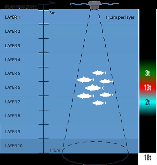
Tuna-AI: tuna biomass estimation with Machine Learning models             A Preprint

in the Indian, Atlantic and Pacific oceans is caught using dFADs, accounting for 36% of the world’s total
tropical tuna catch (Wain et al., 2021; ISSF, 2021).
Initially, dFADs were of natural origin, such as floating logs or objects, that fishermen would come across
while searching for free-swimming schools of tuna. In the mid-1980s, tools began to be developed to allow for
tracking of these dFADs, and fishermen themselves designed purpose-built dFADs that could be attached to
tracking beacons: first based on radar reflectors or radio, and later satellite connected GPS buoys, allowing
the dFADs to be located remotely (Davies et al., 2014; Lopez et al., 2014). The use of these tracking buoys
has been considered “the most significant technological development that has occurred (. . . ) for increasing
the efficiency of dFAD tuna fishing” (Lopez and Scott, 2014). Nowadays, most dFADs are equipped with
satellite-linked instrumented buoys which include both GPS and an echo-sounder, providing fishermen with
accurate geolocation information as well as an estimate of associated tuna biomass. These buoys allow fishing
crews to monitor remotely their dFADs and the biomass they aggregate in real-time, so they can target those
with larger aggregated schools, thus increasing their catch while reducing searching effort (Lopez et al., 2014;
Molina et al., 2003).
The widespread use of dFADs has led to large-scale changes in industrial purse-seine fishing fleets targeting
tropical tunas, affecting traditionally used indices of Catch Per Unit Effort (CPUE) such as search-time and
time-at-sea (Fonteneau et al., 2000). In this context, some authors have highlighted the need for fishery-
independent abundance indices and the use of non-traditional data sources to monitor tuna stock health and
the effects of fishing pressure over time (Baidai et al., 2020; Santiago et al., 2016, 2020). The echo-sounder
buoys attached to dFADs across the world’s oceans can be set to transmit frequent geo-referenced biomass
estimates. Given the number and wide distribution of dFADs in recent years, the information provided by
these echo-sounder buoys could be very valuable. Santiago et al. (2016) presented the first Buoy-Derived
Abundance Index (BAI) for tropical tunas as a proxy of CPUE, based on the biomass estimates provided by
three echo-sounder buoy brands in the Atlantic, Indian and Pacific Oceans.
However, several authors have reported substantial differences between the biomass estimates provided
by echo-sounder buoys and observed biomass (Lopez et al., 2016; Escalle et al., 2019; Orue et al., 2019b),
evidencing the variable nature of fish aggregations under dFADs, often made up of pelagic species other than
tuna (Castro et al., 2002). Likewise, the influence of oceanic conditions on fish distribution and behavior
likely drives aggregation patterns of tuna around dFADs (Lopez, 2017; Druon et al., 2017; Schaefer et al.,
2007). Therefore, in order to develop a representative index of abundance from echo-sounder buoy data, it is
also important to consider and understand the effect of these variables on the biomass estimates given by
these echo-sounder buoys.
Although some studies have already compared biomass estimates from the buoys to catch data (Baidai
et al., 2020; Lopez et al., 2016; Mannocci et al., 2021), the approach in this paper is the first to consider
oceanographic data as predictor variables in Machine Learning models. Likewise, others have combined
oceanographic variables and catch data, without using echo-sounder buoy information (Druon et al., 2017).
Lastly, others have considered the effects of oceanographic conditions on buoy biomass estimates, without
directly comparing it to catch data (Lopez, 2017; Santiago et al., 2020). In this sense, the current study aims
to evaluate several models and methods in order to find which can most accurately estimate biomass under
echo-sounder buoys, combining information from all three sources: catch data, oceanographic variables, and
echo-sounder buoy information, including positional data and biomass estimates.

2       Material and methods
2.1       Database description

Our study draws from three sources of information: activity data on FADs, echo-sounder buoy data, and
oceanography data.

2.1.1       FAD logbook data
The first source of information corresponds to the registered interactions between fishing vessels and echo-
sounder buoys, obtained from the FAD logbooks of the Spanish tropical tuna purse seine fleet operating in
the Atlantic, Indian and Pacific Oceans (2018 - 2020, AGAC2 ship owner’s association data). This FAD
logbook dataset contains almost 66 000 interactions with Satlink buoys. Each record within the dataset can
    2
        Asociación de Grandes Atuneros Congeladores

                                                       2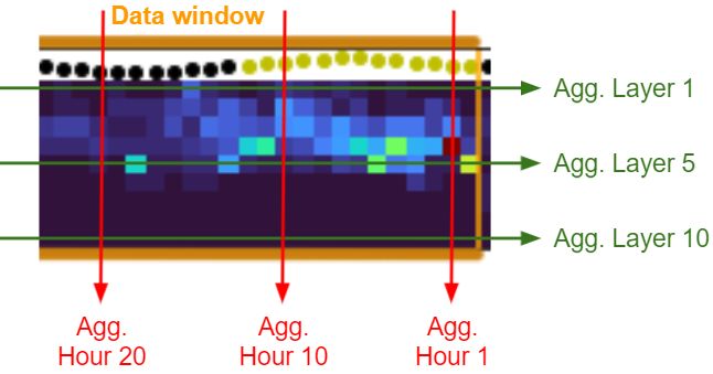
Tuna-AI: tuna biomass estimation with Machine Learning models                 A Preprint

be traced to a specific buoy (using the ID and model of the buoy attached to each dFAD), and contains
information about the date, time and GPS coordinates where the interaction occurred, as well as the nature
of the interaction (see Ramos and et al (2017) for definitions and descriptions of each interaction).
For the purposes of the current study, only events registered as ”Set” and ”Deployment” were used (Ramos
and et al, 2017). Set events, and their associated catch data, were used as “positive cases” and considered
an accurate representation of real tuna biomass under a given dFAD. This follows the assumption that the
entire fish aggregation present at the dFAD is captured by the vessel during the set. This assumption can be
validated by studying the echo-sounder signal before and after the set event. Deployment events were used
as “negative cases”, whereby we consider that no tuna is present under newly deployed dFADs (Orue et al.,
2019a).

2.1.2        Echo-sounder buoy data
The echo-sounder buoy data was collected from 15 497 Satlink buoys3 for which there were registered
interactions in the FAD logbook data (see 2.1.1). This database contained over 68 million records corresponding
to buoys attached to dFADs scattered over the Atlantic, Indian and Pacific Oceans. Each record is referenced
to a specific buoy ID and timestamp, ranging from 2018 to 2020, and contains biomass estimates (explained
below) and GPS coordinates of the buoy’s last known position at the time of measuring. Three buoy models
(ISL+, SLX+ and ISD+) were used in this study, the details of which are described in Table 1. For all buoys,
observation range of the echo-sounder is from 3m to 115m depth, split into ten layers, each with a resolution
of 11.2m (see Figure 1). Biomass estimates (in metric tons, t) are obtained from acoustic samples taken
periodically throughout the day (see Table 1), and the average back-scattered acoustic response is converted
into estimated tonnage, based on the target strength of Skipjack tuna (Katsuwonus pelamis). To reduce the
amount of information to be transmitted, only one measurement per hour is selected, corresponding to that
with the highest estimated tonnage, and sent to the vessel at specific intervals during the day. Thus, the
final temporal resolution of echo-sounder records for each buoy is 1h. The buoys have an internal detection
threshold of 1 ton, which means that a total biomass estimation for any given measurement below 1 ton is
not transmitted and thus interpreted as a zero-reading.

             Model   Echo-sounder      Freq.          Beam               Measuring rate
                                       (kHz)          Angle (◦ )
             ISL+    ES12               190.5         20                 Every 15 minutes
             SLx+    ES16               200           23                 From sunrise to sunset:
                                                                         every 5 minutes
                                                                         From sunset to sunrise: every 60
                                                                         minutes
             ISD+    ES16x2             200 and 38a 23 and 33            From sunrise to sunset:
                                                                         every 5 minutes
                                                                         From sunset to sunrise:
                                                                         every 60 minutes
         a
           Biomass estimates are calculated according to the acoustic response registered by the 200kHz echo-
         sounder, allowing data to be comparable across all buoy models.
                                    Table 1: Buoy models and characteristics

2.1.3        Oceanography data
Oceanographic data was downloaded from the global ocean model (products GLOBAL-ANALYSIS-
FORECAST-PHY-001-024, 1/12◦ resolution; and GLOBAL-ANALYSIS-FORECAST-BIO-001-028, 1/4◦
resolution) provided by the EU Copernicus Marine Environment Monitoring Service4 (Global Monitoring
and Forecasting Center, 2018). For each record contained in the echo-sounder buoy data (see 2.1.2), the
following variables were downloaded: temperature (in ◦ C), chlorophyll-a concentration (in mg/m3 ), dissolved
oxygen concentration (in mmol/m3 ), salinity (in psu), thermocline depth (calculated as the depth where
water temperature is 2◦ C lower than surface temperature, in m), current velocity (in m/s) and sea surface
height anomaly (SSHa, deviation of the sea surface height from long term mean, in m). All variables, except
thermocline and SSHa, were downloaded at surface level (depth = 0.494 m).
   3
       SATLINK, Madrid, Spain, www.satlink.es
   4
       http://marine.copernicus.eu/

                                                           3
Tuna-AI: tuna biomass estimation with Machine Learning models A Preprint
Figure 1: Left: Depth layer configuration and set-up of the Satlink echo-sounder buoys. Right: example of the
biomass estimates (in metric tons) and echogram display available to buoy users. Raw acoustic backscatter is
converted into biomass estimates based on the target strength of skipjack tuna (Katsuwonus pelamis) using
manufacturer’s algorithms.
2.2 Data preprocessing
2.2.1 Data merging
Each set and deployment event registered in the FAD logbook data has been linked to a specific buoy, using
the buoy model and ID. Therefore, each record contained in the echo-sounder buoy database could be related
to a given event. Furthermore, each record contained in the echo-sounder buoy database included the GPS
coordinates of the buoy’s last known position (LKP). Oceanographic information was thus collected for the
date and position of each echo-sounder buoy record. Since oceanographic data are available on a grid with
0.08◦ or 0.25◦ resolution, we incorporate the data from the closest point on the grid to the buoy’s position.
Oceanographic variables change on a larger spatial scale compared to the grid spacing and buoys hourly
movement, so no significant errors are incurred in this approximation.
2.2.2 Echo-sounder window
It is known that tuna schools have well defined circadian behaviours around dFADs that we expect to see
reflected in spatio-temporal patters in the echo-sounder signal. Typically, tuna arrive at dFADs at or near
dawn, and depart around sunset, remaining near the dFAD for several days in a row (Forget et al., 2015;
Dagorn et al., 2007). To capture this regular behaviour, and in order to accurately compare data across time
zones, all echo-sounder and set data was referred to solar time, for which we calculated the sun’s inclination
for each given position and time within the dataset. This also allowed us to calculate the time of sunrise and
sunset per day in the echo-sounder window. There was considerable uncertainty around the time-zone of
registered set and deployment events considered in the FAD logbooks. For this reason, we have chosen to
ignore the time of the event, and keep only the registered event date (see Figure 2).
To relate each set and deployment event to the data included in the echo-sounder buoy dataset, we retrieved
all echo-sounder buoy data on a given window before a set and after a deployment event. Given the periodic
4Tuna-AI: tuna biomass estimation with Machine Learning models A Preprint
behaviour of tuna mentioned previously, we tested the effect of including different length windows of echo-
sounder data on the machine learning models (see 2.3.3) included in our analyses: 24h, 48h and 72h. The
echo-sounder window length with the best results would then be used for all following analyses. For set
events, the last echo-sounder record included in the window corresponds to the sunset on the day prior to the
event. For deployment events, the last echo-sounder record corresponds to 24h, 48h or 72h after sunset on
the day of the last record included in the deployment window (see Figure 2 for an example).
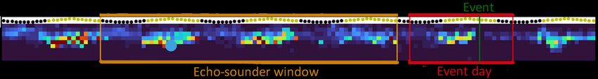
Figure 2: Example of how the 72h echo-sounder window (yellow box) is selected with respect to the event
day (red box). The set event registered in the FAD logbook (assuming UTC) is depicted as a green line. Sun
inclination and day and night patterns are represented above the graph (yellow circles: day; black circles:
night). Colored squares represent the biomass estimates for each measurement from the echo-sounder buoy.
Spatio-temporal patterns of tuna activity are clearly visible in this plot.
2.2.3 Data cleaning
Data used in this study can be quite noisy and it often contains errors, specially event data coming from the
FAD logbook, since it is recorded by persons that tend to approximate the different measurements. For that
reason it is crucial to clean the data to get rid of as many inconsistencies as possible. For a set or deployment
event to be included in the final dataset, the following conditions had to be met:
• The buoy ID registered in the FAD logbook data must match the buoy ID in the echosounder
database, i.e. we ensure that echosounder data are available for the FAD on which the event took
place.
• The echo-sounder window and event day for each buoy (see Figure 2) should not overlap. The reason
to impose this condition is to ensure that inside the window used for prediction there has been no
human intervention on the FAD.
• Following the same procedure as (Escalle et al., 2019), events with invalid positions (i.e. buoys on
land) were removed from the dataset.
• Events or measurements registered at positions with less than 200m water depth were discarded.
This avoids including measurements that are potentially influenced by the sea-bed.
• Using the last known position of the buoys, we computed buoy speed for each position, and dropped
events and measurements where buoy speed was higher than 3 knots, since the surface currents in the
tropical oceans rarely exceed this speed (Orue et al., 2019b). This avoids including measurements
taken on-board a vessel and not representative of a dFAD.
After merging and filtering, the final dataset contained over 12 000 events (see Table 2). These occurred on
10 063 buoys, for which over 665 000 records were collected.
Atlantic Indian Pacific Total
Set 1500 2727 974 5201
Deployment 1369 2199 3426 6994
Total 2869 4926 4400 12 195
Table 2: Number of events remaining after merging echo-sounder and FAD logbook data.
2.3 Model testing
We tested several models using varying feature sets, in order to assess the relative contribution of different
features to model accuracy, as well as test the overall performance of different modelling methods.
5Tuna-AI: tuna biomass estimation with Machine Learning models A Preprint
2.3.1 Feature selection
Based on the merged dataset (see 2.2.1), we considered the variables included in Table 3 as features to be
included in each model. The original biomass measurements form a 10 × {24, 48, 72} matrix, depending on
the echo-sounder window size. These values are not fed directly into the models; instead they are aggregated
both by row (layers) and column (hours) using the maximum, as shown in Figure 3. These aggregations are
then used directly as features for the different models.
As for the number of zero-readings, we just count how many missing records there are in the echo-sounder
window. These missing values are imputed to 0, since the echo-sounder does not transmit any data when the
measurement is below 1t.
Figure 3: Visual example of how the biomass measurements are aggregated.
Echo Echo + Ocean All
Biomass measurements X X X
Number of zero-readings X X X
Buoy model X X X
Chlorophyll-a X X
Dissolved oxygen X X
Salinity X X
Thermocline depth X X
Temperature X X
Current velocity X X
SSHa X X
Day and month X
Year X
Latitude X
Longitude X
Ocean basin X
Sunrise hour X
Sunset hour X
Table 3: Grouped features used for the models. “Echo” includes only data relating to echo-sounder
measurements from the echo-sounder buoy database. “Echo + Ocean” includes oceanography data for the
position and time of each record in the echo-sounder buoy database. “All” contains further derived data from
the position and time of each record in the echo-sounder buoy database.
6Tuna-AI: tuna biomass estimation with Machine Learning models A Preprint
2.3.2 Model selection
Models were trained to achieve three different tasks:
1. A binary classification task, where the target variable y (tuna biomass) can assume the values absent
(y < 10t) or present (y ≥ 10t).
2. A ternary classification task, where the target variable (tuna biomass) can assume the values low
(y < 10t), medium (10t ≤ y < 30t) or high (y ≥ 30t).
3. A regression task, where we directly estimate the tuna biomass y, in tons.
4. A threshold regression task, where we directly estimate the tuna biomass y, in tons, up to a threshold
of 100t. Estimations equal or higher than that were grouped together as ≥ 100t.
The thresholds to define the categories were chosen according to various criteria. In both classification tasks,
the lower threshold was based on best-practice guidelines to decrease shark bycatch, which recommend
avoiding sets on tuna schools less than 10 tons (Restrepo et al., 2016). In the ternary classification task,
the class limit for medium was established according to the median catch (30 tons) in the dataset. In the
threshold regression task, we selected 100 tons since sets above that are relatively rare (315 events, 8.1%).
2.3.3 Machine Learning algorithms and training
Following the usual approach in supervised Machine Learning, we split the dataset into training (75%,
9152 events, 3893 sets and 5259 deployments) and test (25%, 3051 events, 1309 sets and 1742 deployments)
preserving the total class distribution. We considered the performance of a baseline rule-based model and
four different ML models in the classification and regression tasks:
• Baseline: The baseline model only uses the biomass estimates from records contained in the echo-
sounder window (see 2.2.2) for each event. It arrives at an overall biomass estimation by applying a
set of aggregation rules on this matrix. The possible candidates for these aggregation rules are the
sum, the mean and the maximum value. For each task, the selected baseline model was the one with
the best performance.
• Logistic Regression classifier (LR): a linear model for the classification task
• Elastic Net regressor (ENet): for the regression task, with three regularization techniques, namely L1
penalization, L2 penalization and elastic net.
• Random Forest (RF) algorithm (Breiman, 2001).
• Gradient Boosting (GB) algorithm (Friedman, 2001).
• XGBoost (XGB) algorithm (Chen and Guestrin, 2016).
For training and evaluating the models, we used the corresponding algorithms implemented in the python
scikit-learn (Pedregosa et al., 2011) and XGBoost (Chen and Guestrin, 2016) libraries. Each model was
trained on three different sets of predictor variables, listed in Table 3.
2.3.4 Model evaluation
For each model, we performed a grid search with 5-fold cross-validation to find the optimal hyper-parameters.
To select the best set of hyper-parameters for each model, we use the Area Under the Receiver Operating
Characteristic Curve (ROC AUC) for the classification tasks and the Mean Absolute Error (MAE) for the
regression tasks. AUC is defined by plotting the ROC curve (graphing the true positive rate against the false
negative rate at several thresholds) and computing the area below the curve. MAE score is defined as the
average of the absolute values of the errors when comparing the observed and the predicted values.
To report the performance of the models in the classification tasks, we choose the F1 -score, which is the
harmonic mean of precision and recall. For the multi-class task, we report the weighted averaged F1 -score.
3 Results
3.1 Variable echo-sounder window
All GB models, regardless of task, were improved with extended echo-sounder windows. Within the
classification tasks, the best overall results were achieved by the binary classification model (F1 -score = 0.925,
7Tuna-AI: tuna biomass estimation with Machine Learning models A Preprint
Classification (F1 -score) Regression (MAE)
Hours Binary Three class Standard Threshold
24 0.911 0.811 10.16 8.70
48 0.919 0.813 10.05 8.63
72 0.925 0.824 10.03 8.54
Table 4: Model score according to echo-sounder window size for Gradient Boosting regression and classification
models.
Table 4) using the 72h echo-sounder window. Similar results are shown for the regression tasks, where models
using the 72h echo-sounder window had the lowest MAE (Table 4). Of the two regression tasks, the threshold
regression performed better, with MAE almost 1.5 tons lower than standard regression (Table 4).
As echo-sounder windows spanning 72h showed the best result across all models, this is the echo-sounder
window considered in the following analyses.
3.2 Classification tasks
The best performing model in both classification tasks is GB. Performance also increases for every model as
the number of features included in the training increases, i.e. when the models are able to learn from a larger
set of features (Table 5). Thus, the highest overall accuracy score was achieved by the binary task GB model
trained with all features (F1 -score = 0.925, Table 5). The least accurate results were achieved by the ternary
classification Baseline model, which was almost 20% less accurate than the best performing model for this
task, the GB model with all features.
Binary Three class
Models Echo Echo + Ocean All Echo Echo + Ocean All
Baseline 0.754 - - 0.648 - -
LR 0.885 0.889 0.895 0.773 0.788 0.799
RF 0.893 0.911 0.918 0.794 0.799 0.807
XGB 0.900 0.913 0.922 0.798 0.805 0.813
GB 0.907 0.924 0.925 0.791 0.812 0.824
Table 5: F1 -scores for test events (classification task)
When analysing the confusion matrix for the test set of both classification tasks (Figure 4), we see that the
GB model in the binary classification task has a high success rate in classifying whether tuna is present or
absent, misclassifying results in only 6.03% of cases (Figure 4). However, the ternary classification GB model
finds it harder to discriminate between medium (10t ≤ y < 30t) and high (y ≥ 30t) biomass estimations,
having misclassified results in these two classes in 11.14% of cases (Figure 4).
3.3 Regression tasks
Regarding the regression task, the results obtained by all the models trained on the different sets of predictor
variables are shown in Table 6. As in the classification tasks, the GB model for regression tasks also showed
the overall best performance. More specifically, the threshold regression GB model was the most accurate,
achieving a MAE nearly 3 tons lower than the baseline model for the same task, and 1.49 tons lower than the
GB model for the standard regression (Table 6). It is also noteworthy that, as for the classification tasks, all
models benefited from the inclusion of position and oceanography data, and were able to use this information
to improve their predictions with respect to models that were only fed the echo-sounder data.
The mean average error (MAE) shown in Table 6 hides an important fact: the errors are very different for
the two events included in the test set. Indeed, deployment events have by definition an observed biomass of
zero: when tested over deployment events, the GB model has a MAE of 1.23 tons, while the MAE for set
8Tuna-AI: tuna biomass estimation with Machine Learning models A Preprint
Binary classification Ternary classification
1600
1747 69 33
(57.26%) (2.26%) (1.08%)
Low
1400
1738 111
(56.96%) (3.64%)
Absent
1200
1000
True label
True label
52 265 217
(1.70%) (8.69%) (7.11%)
Medium
800
600
73 1129
(2.39%) (37.00%)
Present
37 123 508 400
(1.21%) (4.03%) (16.65%)
High
200
Absent Present Low Medium High
Predicted label Predicted label
Figure 4: Confusion matrices with the performance of the best model on the test set.
Regression Regression (Threshold)
Models Echo Echo + Ocean All Echo Echo + Ocean All
Baseline 12.85 - - 11.40 - -
ENet 13.99 13.70 13.52 12.18 11.84 11.60
RF 10.74 10.30 10.20 9.42 8.93 8.84
XGB 11.37 10.86 10.76 9.60 9.13 9.02
GB 10.51 10.10 10.03 9.18 8.74 8.54
Table 6: MAE scores for test events (regression task)
events is 21.66 tons. The reported overall MAE of 10.03 tons is thus the weighted average of these different
populations. This number is strongly dependent on how the training dataset has been designed (see Table 2).
When looking more closely at the predictions of the best regression model, shown in Figure 5 (left), it
becomes apparent that for very high tuna biomass (y ≥ 100t) the model systematically underestimates tuna
biomass. This result fits well with the improvement mentioned previously of the threshold regression task
in relation to the standard regression. For this model, the MAE over set events drops down to 18.33 tons,
and over deployments it decreases also to 1.18 tons. However, even with this threshold the model tends to
underestimate tuna biomass when observed biomass is high (Figure 5, right). The marginal distributions
for observed and estimated tuna biomass on set events are depicted in Figure 6. Some possible factors that
explain this underestimation are given in Section 4.
4 Discussion
The purpose of this paper is to introduce Tun-AI: a machine learning model for predicting tuna presence,
and/or amount, under echo-sounder buoys attached to dFADs. To achieve this, we tested the performance
of classification and regression methods, as well as the relative impact of including different levels of data
on model performance. The approach used in the current study differs from previous work in that several
models were tested for each task, and our results show that Gradient Boosting was the best model across all
methods. This contrasts with the algorithms and methods applied by previous studies using echo-sounder
data from dFAD buoys to predict the size of tuna aggregations (Baidai et al., 2020; Orue et al., 2019b; Lopez
et al., 2016). However, the assumptions and data-processing methods applied in other work may not be
directly comparable to the process described here. For example, Orue et al. (2019b) or Lopez et al. (2016)
9Tuna-AI: tuna biomass estimation with Machine Learning models A Preprint
250 100
200 80
Estimated tuna biomass y
Estimated tuna biomass y
150 60
100 40
50 20
0 0
0 50 100 150 200 250 0 20 40 60 80 100
Observed tuna biomass y Observed tuna biomass y
Figure 5: Observed tuna biomass against estimated biomass in set events. Scatter plot for the regression task
(left) and density plot for the regression threshold task (right).
0.030
Observed
Estimated
0.025
0.020
Density
0.015
0.010
0.005
0.000
0 20 40 60 80 100 120
Tuna biomass (tons)
Figure 6: Density distributions (set events) of observed and estimated tuna biomass with Gradient Boosting
model.
assume that tunas only occupy layers deeper than 25 m, thus omitting biomass estimates from shallower
layers in their analysis. In our case, all layers were considered, as skipjack tuna are known to prefer warmer
surface waters in areas where the thermocline is shallow (Andrade, 2003). In fact, later studies using the
same approach as Lopez et al. (2016) did not achieve significant improvements on biomass estimates (Orue
et al., 2019c). When developing tuna presence/absence and classification models, Baidai et al. (2020) also
chose to consider all layers in their analyses, which used data from a different brand of echo-sounder buoys in
the Atlantic and Indian oceans, but did not consider oceanographic parameters in their models.
Our analysis also evaluated the impact of oceanographic conditions and position-derived variables on model
performance. Across all tasks and models, the inclusion of additional features improved scores. This
highlights the importance of enriching biomass estimates with contextual information when using data from
echo-sounder buoys attached to dFADs. Previous studies have investigated the relationship between tropical
tuna distribution and oceanographic conditions, both through catch data from observer logbooks and from
dFAD data. For instance, in the Atlantic and Indian oceans skipjack tuna has been known to aggregate
around upwelling systems and productive features where feeding habitat is favorable, and variables such
as sea surface temperature or sea surface height have been shown to have a significant relation with tuna
10Tuna-AI: tuna biomass estimation with Machine Learning models A Preprint
distribution (Druon et al., 2017; Lopez, 2017). In addition, Spanish fishers using echo-sounder buoys on
dFADs consider that the oceanographic context of the dFAD, and the characteristics of each ocean influence
the accuracy of biomass estimates provided by buoys (Lopez and Scott, 2014).
It is worth noting that the oceanographic variables included in the current study were at surface level only
(except for thermocline depth and SSHa). However, given the fact that tuna distribution within the water
column is largely temperature dependent (Aoki et al., 2020; Hino et al., 2019) it is likely that models would
further improve when considering variables depth-wise. Models could be further enriched when considering
dFAD soak time, which has been relevant in previous research, or presence/absence of bycatch species and
other species of tuna (Orue et al., 2019c; Lopez, 2017; Forget et al., 2015). In the current study, species
composition of the catch data was not considered. As the echo-sounder buoys used in this study calculate
biomass estimates based on the target strength of skipjack tuna, it is likely that the presence of other tuna
species such as bigeye, which has a lower target strength (Boyra et al., 2018, 2019), would impact biomass
estimates from the echo-sounder buoys, contributing to errors within the models used to estimate aggregation
size. Most traditional echo-sounder buoys do not currently differentiate between species when giving biomass
estimates, though recent buoy models, such as the ISD+ buoys included in the study, provide a daily estimate
of species composition together with biomass estimates. Although previous studies have highlighted the
importance of considering species composition when estimating biomass (Moreno et al., 2019; Santiago et al.,
2016), the information from these buoys has not yet been applied, and should be considered in future studies.
In the case of classification models, the confusion matrices in Figure 4 showed that most cases where the
model misclassified the tuna aggregation size were when biomass estimates were medium (10t ≤ y < 30t)
or high (y ≥ 30t). On the other hand, when examining the regression models we find that estimated tuna
biomass tended to be lower than observed tuna biomass as the latter increased (Figure 5). This could be due
to various factors: firstly, catches over 100 tons are relatively rare (in our data, 315 events, 8.1%) and thus
the model does not have sufficient examples to properly learn from them; secondly, dFAD buoys are only
able to estimate the biomass of tuna within the echo-sounder beam, and in tuna aggregations over 100 tons
it is unlikely that the entire school is under the buoy at the same time. To resolve this issue, it could be
interesting to apply specialist models which could be adjusted according to when aggregations are predicted
to be small or large. Lastly, it is worth noting that fishermen do not choose on which buoys they set at
random, but based on the raw biomass estimation provided to them, and thus could be biased towards buoys
with higher biomass estimations. This could be a further reason why our ML models underestimate the
observed tuna biomass when its values are above 30t. Future studies exploring the reasons behind fishermen’s
decisions to visit a buoy could provide further insight into this point. This tendency to underestimate should
also be taken into account when using information derived from echo-sounder buoys for stock assessments
(Santiago et al., 2016), although consistent underestimation should have no effect on patterns present in the
temporal series.
The potential applications of accurately quantifying tuna presence or absence around dFADs, as well as school
aggregation size, are numerous. As highlighted by previous authors, data could be used for fishery-independent
abundance indices, improving knowledge on species distribution or better understanding the factors driving
aggregation and disaggregation processes of tuna at dFADs (Santiago et al., 2016; Lopez et al., 2016; Moreno
et al., 2019). The current study represents an important step in this direction, having successfully evaluated
the performance of numerous models on achieving tasks of varying levels of complexity with high degrees of
accuracy. As evidenced here and in previous research, biomass estimates from echo-sounder buoys in and of
themselves provide approximate information on real tuna abundances around dFADs (Lopez et al., 2014).
However, when this massive data is further enriched with remote-sensing data on conditions throughout the
water column and across oceans, and trained with reliable ground-truthed data, Machine Learning proves a
powerful tool for extracting otherwise hidden patterns in the information.
Acknowledgments
This study has been conducted using E.U. Copernicus Marine Service Information. We also thank AGAC
for providing the logbook data used in the analysis and the helpful comments about the manuscript. The
authors would also like to thank Carlos Roa for rendering available the Satlink echosounder dataset. The
research of DGU has been supported in part by the Spanish MICINN under grants PGC2018-096504-B-C33
and RTI2018-100754-B-I00, the European Union under the 2014-2020 ERDF Operational Programme and
the Department of Economy, Knowledge, Business and University of the Regional Government of Andalusia
(project FEDER-UCA18-108393). The research of Manuel Navarro-Garcı́a has been financed by the research
project IND2020/TIC-17526 (Comunidad de Madrid).
11Tuna-AI: tuna biomass estimation with Machine Learning models A Preprint
References
Andrade, H. A. (2003). The relationship between the skipjack tuna (Katsuwonus pelamis) fishery and seasonal
temperature variability in the south-western Atlantic. Fisheries Oceanography, 12(1):10–18.
Aoki, Y., Aoki, A., Ohta, I., and Kitagawa, T. (2020). Physiological and behavioural thermoregulation of
juvenile yellowfin tuna Thunnus albacares in subtropical waters. Marine Biology, 167(6):71.
Baidai, Y., Dagorn, L., Amande, M. J., Gaertner, D., and Capello, M. (2020). Machine learning for
characterizing tropical tuna aggregations under Drifting Fish Aggregating Devices (DFADs) from commercial
echosounder buoys data. Fisheries Research, 229:105613.
Boyra, G., Moreno, G., Orue, B., Sobradillo, B., and Sancristobal, I. (2019). In situ target strength of
bigeye tuna (Thunnus obesus) associated with fish aggregating devices. ICES Journal of Marine Science,
76(7):2446–2458.
Boyra, G., Moreno, G., Sobradillo, B., Pérez-Arjona, I., Sancristobal, I., and Demer, D. A. (2018). Target
strength of skipjack tuna (Katsuwanus pelamis) associated with fish aggregating devices (FADs). ICES
Journal of Marine Science, 75(5):1790–1802.
Breiman, L. (2001). Random Forests. Machine Learning, 45(1):5–32.
Castro, J. J., Santiago, J. A. J., and Santana-Ortega, A. T. (2002). A general theory on fish aggregation to
floating objects: An alternative to the meeting point hypothesis. Reviews in Fish Biology and Fisheries,
11(3):24.
Chen, T. and Guestrin, C. (2016). {XGBoost}: A Scalable Tree Boosting System. In Proceedings of the
22nd ACM SIGKDD International Conference on Knowledge Discovery and Data Mining, KDD ’16, pages
785–794, New York, NY, USA. ACM.
Dagorn, L., Holland, K. N., and Itano, D. G. (2007). Behavior of yellowfin (Thunnus albacares) and bigeye
(T. obesus) tuna in a network of fish aggregating devices (FADs). Marine Biology, 151(2):595–606.
Davies, T. K., Mees, C. C., and Milner-Gulland, E. J. (2014). The past, present and future use of drifting
fish aggregating devices (FADs) in the Indian Ocean. Marine Policy, 45:163–170.
Druon, J. N., Chassot, E., Murua, H., and Lopez, J. (2017). Skipjack tuna availability for purse seine fisheries
is driven by suitable feeding habitat dynamics in the Atlantic and Indian Oceans. Frontiers in Marine
Science, 4(OCT):315.
Escalle, L., Heuvel, B. V., Clarke, R., Brouwer, S., Pilling, G., Lauriane Escalle, Heuvel, B. V., Clarke, R.,
Brouwer, S., and Pilling, G. (2019). Report on preliminary analyses of FAD acoustic data. Western and
Central Pacific Fisheries Commission, 53(9):17.
Fonteneau, A., Pallarés, P., and Pianet, R. (2000). A worldwide review of purse seine fisheries on FADs.
Regional syntheses, page 21.
Forget, F. G., Capello, M., Filmalter, J. D., Govinden, R., Soria, M., Cowley, P. D., and Dagorn, L. (2015).
Behaviour and vulnerability of target and non-target species at drifting fish aggregating devices (FADs) in
the tropical tuna purse seine fishery determined by acoustic telemetry. Canadian Journal of Fisheries and
Aquatic Sciences, 72(9):1398–1405.
Friedman, J. H. (2001). Greedy function approximation: A gradient boosting machine. Annals of Statistics,
29(5):1189–1232.
Global Monitoring and Forecasting Center (2018). Operational Mercator global ocean analysis and forecast
system, E.U. Copernicus Marine Service Information. https://resources.marine.copernicus.eu (Accessed:
15th January 2021).
Hino, H., Kitagawa, T., Matsumoto, T., Aoki, Y., and Kimura, S. (2019). Changes to vertical thermoregulatory
movements of juvenile bigeye tuna (Thunnus obesus) in the northwestern Pacific Ocean with time of day,
seasonal ocean vertical thermal structure, and body size. Fisheries Oceanography, 28(4):359–371.
ISSF (2021). Status of the World Fisheries for Tuna. Mar 2021. ISSF Technical Report 2021-10, March
2021(March):1–120.
Lopez, J. (2017). Environmental preferences of tuna and non-tuna species associated with drifting fish
aggregating devices (DFADs) in the Atlantic Ocean, ascertained through fishers’ echo-sounder buoys.
Deep–Sea Research II, page 12.
Lopez, J., Moreno, G., Boyra, G., and Dagorn, L. (2016). A model based on data from echosounder buoys to
estimate biomass of fish species associated with fish aggregating devices. Fishery Bulletin, 114(2):166–178.
12Tuna-AI: tuna biomass estimation with Machine Learning models A Preprint
Lopez, J., Moreno, G., Sancristobal, I., and Murua, J. (2014). Evolution and current state of the technology
of echo-sounder buoys used by Spanish tropical tuna purse seiners in the Atlantic, Indian and Pacific
Oceans. Fisheries Research, 155:127–137.
Lopez, J. and Scott, G. P. (2014). The use of FADs in tuna fisheries. European Union, 1(February):70.
Mannocci, L., Baidai, Y., Forget, F., Tolotti, M. T., Dagorn, L., and Capello, M. (2021). Machine learning to
detect bycatch risk: Novel application to echosounder buoys data in tuna purse seine fisheries. Biological
Conservation, 255(February):109004.
Maufroy, A., Chassot, E., Joo, R., and Kaplan, D. M. (2015). Large-Scale Examination of Spatio-Temporal
Patterns of Drifting Fish Aggregating Devices (dFADs) from Tropical Tuna Fisheries of the Indian and
Atlantic Oceans. PLOS ONE, 10(5):e0128023.
Molina, D. D., Pallares, P., Areso, J. J., and Ariz, J. (2003). Statistics of the purse seine spanish fleet in the
Indian Ocean (1984-2002). IOTC Proceedings no. 2, 6(6):115–128.
Moreno, G., Boyra, G., Sancristobal, I., Itano, D., and Restrepo, V. (2019). Towards acoustic discrimination
of tropical tuna associated with Fish Aggregating Devices. PLOS ONE, 14(6):e0216353.
Orue, B., Lopez, J., Moreno, G., Santiago, J., Boyra, G., Soto, M., and Murua, H. (2019a). Using fishers’
echo-sounder buoys to estimate biomass of fish species associated with drifting fish aggregating devices in
the Indian Ocean. Revista de Investigación Marina, 26(1):3–12.
Orue, B., Lopez, J., Moreno, G., Santiago, J., Boyra, G., Uranga, J., and Murua, H. (2019b). From fisheries
to scientific data: A protocol to process information from fishers’ echo-sounder buoys. Fisheries Research,
215(February):38–43.
Orue, B., Lopez, J., Moreno, G., Santiago, J., Soto, M., and Murua, H. (2019c). Aggregation process of
drifting fish aggregating devices (DFADs) in the Western Indian Ocean: Who arrives first, tuna or non-tuna
species? PLOS ONE, 14(1):e0210435.
Pedregosa, F., Varoquaux, G., Gramfort, A., Michel, V., Thirion, B., Grisel, O., Blondel, M., Prettenhofer,
P., Weiss, R., Dubourg, V., Vanderplas, J., Passos, A., and Cournapeau, D. (2011). Scikit-learn: Machine
Learning in Python. Machine Learning in Python, page 6.
Ramos, M. L. and et al (2017). Spanish FADs logbook: solving past issues, responding to new global
requirements. 1st Ad-Hoc IOTC Working Group on FADs, 2017(April):1–24.
Restrepo, V., Dagorn, L., and Moreno, G. (2016). Mitigation of Silky Shark Bycatch in Tropical Tuna Purse
Seine Fisheries. ISSF Technical Reportl Report.
Santiago, J., Lopez, J., Moreno, G., Quincoces, I., Soto, M., and Murua, H. (2016). Towards a Tropical Tuna
Buoy-derived Abundance Index (TT-BAI). Collect. Vol. Sci. Pap. ICCAT, 72(3):714–724.
Santiago, J., Uranga, J., Quincoces, I., Grande, M., and Murua, H. (2020). A Novel Index of Abundance
of Skipjack in the Indian Ocean Derived From Echosounder Buoys. Collect. Vol. Sci. Pap. ICCAT,
76(6):321–343.
Schaefer, K. M., Fuller, D. W., and Block, B. A. (2007). Movements, behavior, and habitat utilization of
yellowfin tuna (Thunnus albacares) in the northeastern Pacific Ocean, ascertained through archival tag
data. Marine Biology, 152(3):503–525.
Wain, G., Guéry, L., Kaplan, D. M., and Gaertner, D. (2021). Quantifying the increase in fishing efficiency
due to the use of drifting FADs equipped with echosounders in tropical tuna purse seine fisheries. ICES
Journal of Marine Science, 78(1):235–245.
13Tuna-AI: tuna biomass estimation with Machine Learning models A Preprint
Appendices
A Classification task categories
When defining the categories for the classification task, the thresholds were chosen according to various
criteria. In both binary and ternary tasks, the lower threshold was based on best-practice guidelines to
decrease shark bycatch, which recommend avoiding sets on tuna schools less than 10 tons (Restrepo et al.,
2016). In the ternary classification task, the class limit for medium was established according to the median
catch (30 tons) in the dataset (see Figure 7).
2000
Mean: 41.9 tons
1750 Quantile 25: 15.0 tons
Quantile 50: 30.0 tons
1500 Quantile 75: 50.0 tons
1250
Frequency
1000
750
500
250
0
0 50 100 150 200 250 300 350 400
Catch (tons)
Figure 7: Distribution of caught tons of tuna, from a total of 5202 set events.
B Feature importance
An always challenging task in ML projects is their interpretability: to understand to some extent which
features is the model mostly paying attention to. There exist several approaches to assess feature importance,
and in this work we employ permutation importance (Breiman, 2001), which evaluates the importance of a
given feature as the drop in model’s efficiency when the values of that column are shuffled randomly in the
training set.
In Table 7 we rank the 10 most important features for each task, based on the GB model. We explain next
the meaning of each feature:
• Agg.T is the aggregated value of the 72 × 10 echo-sound array.
• N NaN is the number of missing records, ranging from 0 to 72.
• Agg.LY is obtained by aggregating the 72 values at layer Y, where layer 1 is the closest to the surface.
• Agg.HX is obtained by aggregating the 10 values at hour X, where 0 is the closest to the event.
• O2.X and Zos.X are the dissolved oxygen and sea surface height, respectively, at hour X. As oceanog-
raphy features are recorded daily, X can only take values 0, 23, 47 and 71 for these two variables.
• Latitude and Longitude are the buoy coordinates at hour 0.
• Ocean is a categorical variable that indicates the ocean where the event took place.
14Tuna-AI: tuna biomass estimation with Machine Learning models A Preprint
Classification Regression
Rank Binary Three class Standard Threshold
1 Agg.L5 Agg.L5 Agg.T Agg.T
2 Longitude Longitude Agg.L5 Agg.L5
3 Ocean Ocean Longitude Longitude
4 N NaN Agg.L2 Latitude Agg.L2
5 Latitude Agg.H10 Agg.H32 Zos.0
6 Agg.L7 Zos.0 Agg.L2 Latitude
7 Agg.L1 Latitude Zos.0 Agg.L6
8 Agg.L6 Zos.71 Agg.H35 Zos.23
9 Agg.T O2.23 Zos.23 Zos.71
10 Agg.L2 O2.0 Zos.71 Agg.H10
Table 7: Top ten most important features for the GB model in each of the 4 tasks. The variables are
coloured depending on the feature group they belong. Blue corresponds to acoustic features, green refers to
oceanografic variables and red identifies geographical coordinates (or features derived from them)
Interpretation of feature importance must be exercised with care, since there are clearly correlations among
the variables, and this has to be taken into account when interpreting permutation importance.
C Hyper-parameter search
A grid search with cross-validation has been conducted to find the best hyper-parameters for each model by
maximizing the ROC AUC. The hyper-parameter grid for all the models using the full set of features in each
of the four tasks is shown in Tables 8, 10 and 9. For Logistic Regression and Elastic Net, a grid search was
conducted using the standard classes LogisticRegressionCV and ElasticNetCV, with a l1 ratio grid of
[0.0, 0.2, 0.4, 0.6, 0.8, 1.0] and [0.1, 0.5, 0.9, 1.0] respectively. The final values selected by cross-validation
were 1 and 0.9. The name of the hyper-parameters coincide with the names that they have in Scikit-Learn’s
(Pedregosa et al., 2011)the implementation. All the parameters not shown here were set to its default value
(see the documentation for more details). Finally, the set of optimal hyper-parameters for each of the models
is shown in Tables, 11, 13 and 12.
Parameter Classification Regression
n estimators [200, 500, 1000] [100, 200, 500]
max samples [None, 0.8] [None, 0.8]
max depth [None, 2, 4] [None, 4, 8]
min samples split [2, 8, 32] [2, 8, 32]
min samples leaf [1, 4, 16] [1, 4, 16]
max features [None, sqrt, log2] [None, sqrt, log2]
Table 8: Grid of hyper-parameters used in the Random Forest models.
Parameter Classification Regression
n estimators [50, 100, 200] [400]
learning rate [0.01, 0.1, 0.2] [0.01, 0.1, 0.2]
max depth [None, 3, 6] [None, 3, 6]
min samples split [2, 4, 8] [2, 4, 8]
min samples leaf [1, 2, 4] [1, 2, 4]
max features [None, sqrt, log2] [None, sqrt, log2]
Table 9: Grid of hyper-parameters used in the Gradient Boosting models.
15Tuna-AI: tuna biomass estimation with Machine Learning models A Preprint
Parameter Classification Regression
n estimators [50] [50, 100, 200]
learning rate [0.2] [0.01, 0.1, 0.2]
max depth [2, 4] [2, 4, 6]
subsample [1.0] [0.7, 1.0]
colsample bytree [1.0] [0.5, 1.0]
Table 10: Grid of hyper-parameters used in the XGBoost models.
Classification Regression
Parameter Binary Three class Standard Threshold
n estimators 1000 500 100 200
max samples None None None None
max depth None None None None
min samples split 2 8 8 2
min samples leaf 1 1 4 4
max features sqrt sqrt None None
Table 11: Best hyper-parameters for the Random Forest models trained on all features.
Classification Regression
Parameter Binary Three class Standard Threshold
n estimators 200 200 400 400
learning rate 0.2 0.1 0.01 0.01
max depth 6 6 None None
min samples split 8 2 2 4
min samples leaf 4 2 4 8
max features log2 log2 auto auto
Table 12: Best hyper-parameters for the Gradient Boosting models trained on all features.
Classification Regression
Parameter Binary Three class Standard Threshold
n estimators 50 50 200 200
learning rate 0.2 0.2 0.01 0.01
max depth 4 4 6 6
subsample 1.0 1.0 0.7 0.7
colsample bytree 1.0 1.0 0.5 0.5
Table 13: Best hyper-parameters for the XGBoost models trained on all features.
16You can also read