LIDAR OBSERVATIONS OF MULTI-MODAL SWASH PROBABILITY DISTRIBUTIONS ON A DISSIPATIVE BEACH - MDPI
←
→
Page content transcription
If your browser does not render page correctly, please read the page content below
remote sensing
Article
LiDAR Observations of Multi-Modal Swash Probability
Distributions on a Dissipative Beach
Caio Eadi Stringari *,†,‡                  and Hannah E. Power ‡

                                             School of Environmental and Life Sciences, University of Newcastle, 2308 Newcastle, Australia;
                                             hannah.power@newcastle.edu.au
                                             * Correspondence: Caio.EadiStringari@uon.edu.au
                                             † Current address: France Energies Marines, 29280 Plouzané , France.
                                             ‡ These authors contributed equally to this work.

                                             Abstract: Understanding swash zone dynamics is of crucial importance for coastal management as the
                                             swash motion, consisting of the uprush of the wave on the beach face and the subsequent downrush,
                                             is responsible for driving changes in the beach morphology through sediment exchanges between
                                             the sub-aerial and sub-aqueous beach. Improved understanding of the probabilistic characteristics of
                                             these motions has the potential to allow coastal engineers to develop improved sediment transport
                                             models which, in turn, can be further developed into coastal management tools. In this paper,
                                             novel descriptors of swash motions are obtained by combining field data and statistical modelling.
                                             Our results indicate that the probability distribution function (PDF) of shoreline height timeseries
                                             (p(ζ )) and trough-to-peak swash heights (p(ρ)) measured at a high energy, sandy beach were both
                                             inherently multimodal. Based on the observed multimodality of these PDFs, Gaussian mixtures
                                             are shown to be the best method to statistically model them. Further, our results show that both
                                             offshore and surf zone dynamics are responsible for driving swash zone dynamics, which indicates
                                             unsaturated swash. The novel methods and results developed in this paper, both data collection and
                                   analysis, could aid coastal managers to develop improved swash zone models in the future.


Citation: Stringari, C.E.; Power, H.E.       Keywords: LiDAR; swash zone; nearshore waves; probability distributions; sandy beaches
LiDAR Observations of Multi-Modal
Swash Probability Distributions on a
Dissipative Beach. Remote Sens. 2021,
13, 462. https://doi.org/10.3390/
                                             1. Introduction
rs13030462
                                                  The swash zone encompasses the transition region between the sub-aqueous and
Academic Editor: Chris Blenkinsopp           the sub-aerial beach [1]. It is a highly dynamic environment with alternating wet and
Received: 20 December 2020                   dry conditions. Over the past five decades, this region has attracted increased research
Accepted: 26 January 2021                    interest due to the significant role it plays in sediment dynamics and beach erosion [2].
Published: 28 January 2021                   The cross-shore shoreline oscillation, globally referred to as swash, can be divided into two
                                             main components: the uprush of the wave on the beach face and the subsequent downrush.
Publisher’s Note: MDPI stays neu-            Each of these two divisions can be described by their horizontal and vertical (height)
tral with regard to jurisdictional clai-     components (Figure 1). A large proportion of swash zone research has focused on obtaining
ms in published maps and institutio-         empirical parametric formulae to describe extreme runup heights (see Atkinson et al. [3]
nal affiliations.                            and Power et al. [4] for recent reviews); however, as highlighted by Hughes et al. [5], this
                                             approach may not be fully satisfactory to provide information to coastal managers to
                                             develop operational tools other than inundation models.
Copyright: © 2021 by the authors. Li-
                                                  The natural variability of the probability distribution functions (PDFs) of swash
censee MDPI, Basel, Switzerland.
                                             motions has received little research attention to date. To the authors’ knowledge, only
This article is an open access article
                                             two studies have attempted to describe the variability of these PDFs in detail [5,6], both of
distributed under the terms and con-         which compared measured swash maxima PDFs to Cartwright and Longuet-Higgins’ [7]
ditions of the Creative Commons At-          theoretical PDF for the maxima of a random variable. This theoretical PDF is a direct
tribution (CC BY) license (https://          function of the spectral width (ϕ) of the analysed timeseries and reduces to the Rayleigh
creativecommons.org/licenses/by/             PDF for narrow bandwidth processes (ϕ = 0) or to the Gaussian PDF for wide bandwidth
4.0/).                                       processes (ϕ = 1). Holland and Holman [6] found that their measured swash maxima PDFs

Remote Sens. 2021, 13, 462. https://doi.org/10.3390/rs13030462                                           https://www.mdpi.com/journal/remotesensing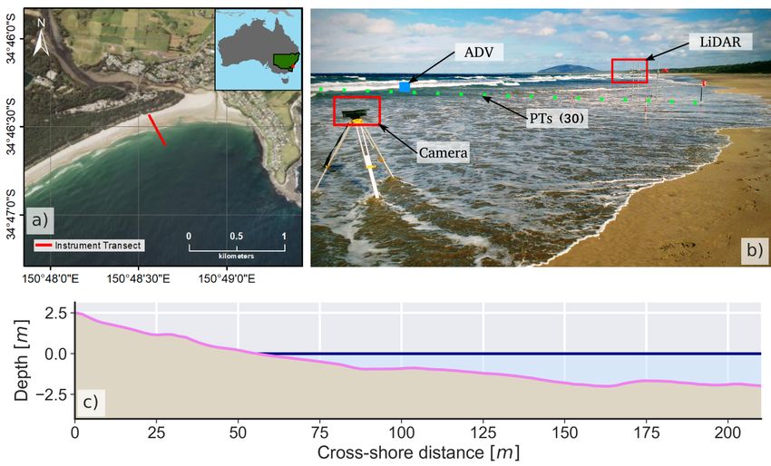
Remote Sens. 2021, 13, 462                                                                                                         2 of 16

                                  matched Cartwright and Longuet-Higgins’ [7] PDF for some values of ϕ, but they could
                                  not directly correlate the variability in their PDFs to environmental parameters. It has
                                  been observed [8], however, that the spectral width parameter ϕ does not correlate with
                                  wave height PDFs in the surf zone and, by induction, should not correlate with swash
                                  heights either. More recently, Hughes et al. [5] investigated the PDFs of the shoreline height
                                  timeseries (p(ζ )) and trough-to-peak runup heights (p(ρ)), in addition to swash maxima
                                  PDFs. They observed that, on average, observed p(ζ ) PDFs were consistently right skewed
                                  when compared to the Gaussian PDF predicted by Longuet-Higgins [9], possibly due to the
                                  broad-band wave spectrum observed on natural beaches. Further, these authors compared
                                  p(ρ) with both the Rayleigh and Gaussian PDFs but neither of these PDFs seemed to
                                  satisfactorily describe their observations (see Figure 6 in Hughes et al. [5], for example).

      Figure 1. Swash zone definitions. Note that runup is defined relative to the still water level (SWL), the shoreline height (or
      elevation, ζ) is defined centred on the mean water level (MWL), and the trough-to-peak swash height (ρ) is defined for each
      swash cycle. Here, each swash cycle was defined by a local minima analysis.

                                       In this paper, we provide novel field observations of swash motion PDFs obtained
                                  from a high-resolution LiDAR system deployed at a high-energy sandy beach and test the
                                  hypothesis that well defined, uni-variate and uni-modal PDFs (for example, the Gaussian
                                  PDF) are able to describe observed swash zone data. Specifically, the statistical properties of
                                  shoreline height timeseries (ζ) and trough-to-peak swash height (ρ) PDFs are investigated
                                  in detail. In addition, detailed surf zone and offshore data are used to the assess the
                                  patterns observed in the swash zone. The results obtained here deviate significantly from
                                  the theoretical predictions from Longuet-Higgins [9] for the analysis of p(ζ ) and do not
                                  support the concept of swash saturation [10]. The present data indicate that a combination
                                  of surf zone and offshore forcing control swash zone dynamics. Finally, an approach that
                                  allows offshore and surf zone parameters be linked to the variability of p(ζ ) is investigated.
                                  This paper is organised as follows. Section 2 describes the data collection methods and
                                  pre-processing, Section 3 presents the results of the field data collection with a focus on
                                  probabilistic descriptors for swash, Section 4 discusses the results, and Section 5 concludes.

                                  2. Materials and Methods
                                  2.1. Data Collection
                                       Data were collected at Seven Mile Beach, Gerroa, New South Wales, Australia, here-
                                  after SMB. This beach is classed as modally dissipative in the Australian morphodynamic
                                  beach model [11,12] and for the duration of the present experiment, was characterised by a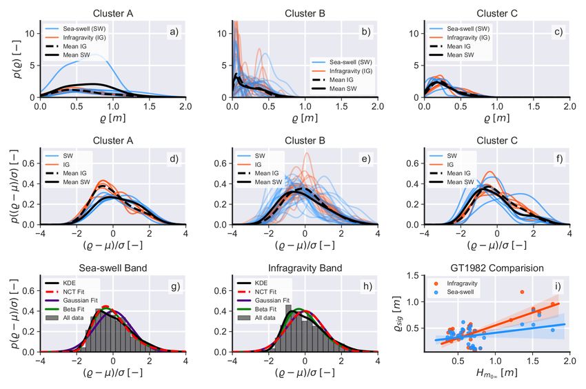
Remote Sens. 2021, 13, 462                                                                                                  3 of 16

                                 gently sloping profile (with slope β = 0.03) with no significant barred morphology, beach
                                 cusps, or alongshore variability. Video imagery, pressure transducer (PT), offshore spec-
                                 tral wave, Light imaging Detection And Ranging (LiDAR), acoustic Doppler velocimeter
                                 (ADV), and topographic data were collected during a field data collection experiment over
                                 six days in June 2018. In this paper, the focus will be on the LiDAR , surf zone (PT) and
                                 offshore data. The experimental design is shown in Figure 2 and is summarised below. See
                                 Stringari et al. [13] and Stringari and Power [14] for further details.
                                       The PT data collection consisted of 30 PTs (RBR Solo and INW P2X ) deployed on the
                                 seabed in a cross-shore orientation. The LiDAR (SiCK LMS511) was mounted on a scaffold
                                 frame and recorded in the same cross-shore orientation as the PT transect (see Figure 2a,b).
                                 The ADV (Sontek Hydra) was deployed approximately 50 m seaward of the LiDAR. The
                                 Datawell waverider buoy was deployed offshore of the transect line at the 10 m isobath.
                                 Two video cameras were used: a Sony camera (HDR-CX240)
                                       mounted at Gerroa headland and a Raspberry-Pi-based system [15] mounted directly
                                 facing the LiDAR (shown in Figure 2b). The beach was surveyed several times each day
                                 using a Trimble S5 total station and a Trimble R4 RTK GPS, and the representative beach
                                 profile is shown in Figure 2c. Figure 3 shows the offshore conditions for the duration of
                                 the field campaign. This dataset was ultimately chosen for the analyses presented in this
                                 paper because it overcomes the limitations of classical remote-sensing datasets (e.g., pixel
                                 misregistration; see Vousdoukas et al.’s [16] Figure 7), it has precise and unique offshore
                                 conditions, and it has a high degree of offshore wave variability for comparable tidal water
                                 levels and beach slopes.

      Figure 2. (a) Experiment location. The red line shows the instrumentation transect. (b) Photo of the experimental setup
      (19/06/2018). (c) Representative beach profile (16/08/2018).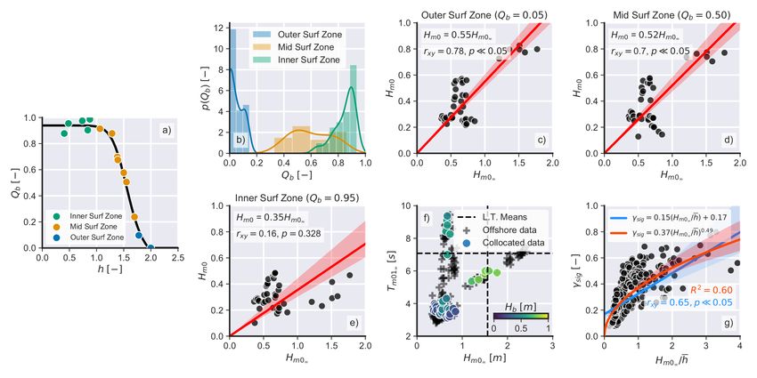
Remote Sens. 2021, 13, 462 4 of 16
Figure 3. Offshore data (spectral significant wave heights, Hm0∞ , and periods, Tm01∞ ), for the duration of the field
campaign. The filled blue regions indicate periods of simultaneous offshore, Light imaging Detection And Ranging (LiDAR),
and pressure transducer (PT) data collection.
2.2. Data Processing
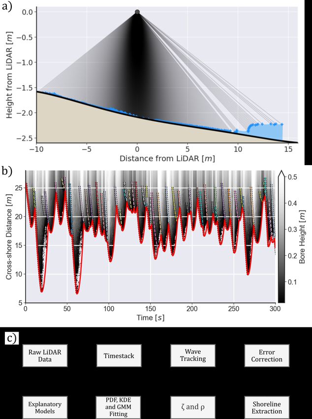
From the raw LiDAR data (Figure 4a), timeseries of the cross-shore evolution of
the water surface elevation were extracted at 10 Hz and stacked in time, resulting in
a dataset similar to a video-derived timestack [17] (Figure 4b, color scale). Incoming
waves were tracked using a modified version of the method from Stringari, Harris, and
Power [13]. For each LIDAR timestack, the vertical Sobel [18] edge detector was applied
to the timestack, and pixel intensity peaks in the resulting image were extracted and then
clustered using the DBSCAN algorithm [19]. Unlike the original method, no colour-based
machine learning was applied to the dataset. The absence of the colour-learning step
resulted in a significant increase in the number of false-positive cases of wave crests being
detected. These erroneous wave crests were manually corrected in QGIS (version 10.4) to
ensure that no errors were propagated into subsequent analyses. Optimal wave paths were
then obtained as per the original tracking algorithm [13]. The tracking algorithm was set to
stop tracking waves if the water elevation above the bed was less than 0.015 m, which is
significantly lower than other recent works [20,21]. Note that in this paper, we have not
quantified uncertainties related to the raw LiDAR data; future research should, however,
focus on developing methods to quantify and correct for such uncertainties.
The temporal evolution of the shoreline position was obtained in three steps: (1) the
uprush was obtained from the tracked wave paths as described above, (2) the downrush
was obtained via edge detection using the horizontal Sobel [18] operator, and (3) the
continuous shoreline timeseries was obtained by combining the results of steps (1) and (2)
and interpolating the data to a regular time vector with a sample frequency of 5 Hz using a
Gaussian radial basis function (RBF) interpolation. Finally, horizontal shoreline excursion
timeseries were converted to shoreline height (ζ) timeseries and to trough-to-peak swash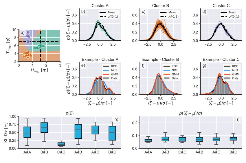
Remote Sens. 2021, 13, 462                                                                                                          5 of 16

                                   heights (ρ) using the measured beach profiles and a local minima analysis (see Figure 1 for
                                   definitions). The Australian Height Datum (AHD, [22]) was used as the vertical reference.

      Figure 4. (a) Raw LiDAR data showing a bore running up the beach profile. (b) Example of LiDAR timestack showing the
      tracked wave paths (coloured dashed lines) and the resulting time-varying shoreline position (thick red line). The grey
      scale indicates the bore height (that is, water depth) in relation to the measured profile in (a). (c) Flowchart indicating the
      methodological steps used in this paper.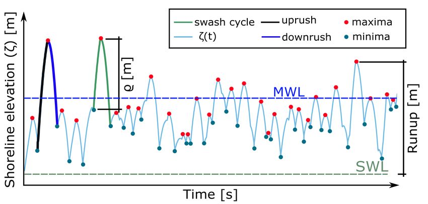
Remote Sens. 2021, 13, 462                                                                                            6 of 16

                             3. Results
                             3.1. Surf Zone Dynamics
                                   The cross-shore variation of surf zone significant wave heights (Hm0 ) and the fraction
                             of broken waves (Qb ) were used to assess the surf zone dynamics (Figure 5). In this paper,
                             Qb was calculated as follows: for each data run in which there were unique offshore, surf
                             zone, and swash zone data available, 10 min of PT data were extracted from the raw records
                             and, from these records, individual waves were extracted using a local minima analysis as
                             per Power et al. [23] and classified as broken or unbroken using the neural network from
                             Stringari and Power [14]. The neural network was updated with field data from Seven
                             Mile Beach to increase the classification performance for the present dataset. The updated
                             neural network accuracy score reached 95% when classifying waves in a test dataset (that
                             is, data that the neural network had never seen) and correlation scores (r2 ) were >0.95 for
                             Qb predictions (not shown).
                                   Data from each Qb curve were segmented into three clusters using the k-means algo-
                             rithm (Figure 5a): one cluster that was representative of the outer surf zone, one cluster
                             representative of the mid surf zone, and one cluster representative of the inner surf zone.
                             The probability distribution of Qb (p( Qb )) was then calculated for each class (Figure 5b),
                             which showed that in the outer surf zone, most of the waves were unbroken (p( Qb ) < 0.2);
                             in the mid surf zone, about half of the waves were broken (p( Qb ) ≈ 0.5); and in the
                             inner surf zone, most waves were broken (p( Qb ) > 0.8). This result is consistent with
                             the conceptual hydro-kinematic model for gently sloping beaches [24]. Interestingly, Qb
                             values close to the surf–swash boundary were never Qb = 1, which indicates that small
                             unbroken waves reach the swash zone, even on a dissipative beach such as SMB (average
                                                               tan β
                             Iribarren Number [25] ξ ∞ = √             = 1.21, where L∞ is the wave length calculated as
                                                               Hm0∞ L∞
                                     g 2                              Hm
                             L∞ =   2π Tm01∞ , and averaged   Ω∞ = Tm 0∞Ws  = 3.77, where Ws is the sediment fall velocity).
                                                                       01∞
                             Based on the observed distributions of Qb , three locations in the surf zone were chosen to
                             assess wave heights: Qb = 0.95 (inner surf zone), Qb = 0.50 (mid surf zone), and Qb = 0.05
                             (outer surf zone).
                                  The analysis of the correlation between offshore (Hm0∞ ) and surf zone (Hm0 ) wave
                             heights showed that there was a direct correlation between Hm0 and Hm0∞ across the full
                             width of the surf zone (Figure 5c–f). Following the definition of surf zone saturation
                             from Power et al. [26], the observed correlations strongly suggest that the surf zone was
                             unsaturated during the experiment, despite the dissipative nature of the beach. Finally,
                             the wave-height-to-water-depth ratio (γsig ) was compared to the offshore wave height
                             normalised by averaged water depth for each 10 min data run (Hm0∞ /h) (Figure 5g).
                             The results from this analysis are analogous to Figure 11 in Power et al. [23] and indicate
                             that (1) the surf zone was unsaturated and (2) there was a terminal bore height reaching
                             the surf–swash boundary. Following from the analysis in Figure 5a that Qb 6= 1, this
                             terminal bore height could represent either broken or unbroken waves. These results are
                             significant because if the surf zone is unsaturated, it is probable that the swash zone is also
                             unsaturated. This is discussed further in Section 4.
Remote Sens. 2021, 13, 462 7 of 16
Figure 5. (a) Example of Qb curve segmentation using k-means for one 10 min data run. (b) Algorithm clustered Qb probability distribution functions (PDFs). The number of bins for these
histograms was calculated using the Freedman and Diaconis [27] rule. Correlations between offshore (Hm0∞ ) and surf zone (Hm0 ) wave heights in (c) the outer surf zone, (d) the mid surf
zone, and (e) the inner surf zone. The red swath shows the 95% confidence interval for the linear regression. (f) Comparison between offshore conditions (Hm0∞ and Tm01∞ ) and break
point wave height (Hb ). The crosses show all the measured offshore data, and the dashed lines show the long-term Hm0∞ and Tm01∞ averages for the nearest offshore wave buoy (Port
Kembla) [28]. (g) Analysis of γsig against Hm0∞ /h (analogous to Figure 11 in Power et al. [23]). The coloured swaths show the 95% confidence interval for the regressions.Remote Sens. 2021, 13, 462 8 of 16
3.2. Shoreline Height Timeseries PDFs
For each data run in which there were unique offshore and LiDAR data, 10 min
timeseries were extracted from the raw LiDAR record and the time-varying shoreline was
obtained using the method described in Section 2.2. The PDFs of normalised (p((ζ − µ)/σ ))
and non-normalised (p(ζ )) shoreline height timeseries were then obtained via histograms
and kernel density estimations (KDEs). The use of KDEs to obtain PDFs is advantageous
over more traditional histogram methods because (1) they are a fully non-parametric
approach, and (2) they are able to identify fluctuations in the data’s distribution that are
usually not seen when using histograms with potentially non-ideal bin sizes.
Analysis of individual normalised shoreline height PDFs indicated a high degree
of variability between runs and that the majority of PDFs were multimodal (97.5%).
The Shapiro and Wilk [29] test at the 95% confidence interval confirmed that none of
the analysed timeseries were normally distributed. The observed PDFs were then grouped
into three clusters based on the observed offshore conditions (Figure 6a). Cluster A rep-
resents average wave height conditions with short periods, Cluster B represents calm
conditions (low wave heights and short wave periods), and cluster C represents calm
conditions with long wave periods. Figure 6b shows the PDFs for cluster A, Figure 6c
shows the PDFs for cluster B, and Figure 6d shows the PDFs for cluster C. By averaging
the PDFs in each cluster, a right-skewed PDF similar to Hughes et al.’s [5] ensemble PDF
was observed (see their Figure 2). To assess the effect of the normalisation strategy and
offshore conditions on the shape of the shoreline height PDFs, each PDF was compared to
every other PDF in the same cluster, and then to every PDF in each of the other two clusters
using the Kullback and Leibler [30] divergence as the similarity measurement. The results
from this analysis indicated that (1) non-normalised PDFs (p(ζ )) are dissimilar within and
between clusters (Figure 6h), except PDFs in cluster C, which are strongly similar to each
other, and (2) normalised PDFs (p((ζ − µ)/σ )) are strongly similar within and between
clusters (Figure 6i). For further discussion see Section 4.
Two other methods were assessed for obtaining a function (or combination of func-
tions) to describe the observed PDFs. This was done because KDE is a non-parametric
method that requires prior knowledge of the input timeseries, thus preventing an as-
sessment of correlations between descriptors of the analysed PDFs and environmental
parameters. Note that the results presented below were invariant regardless of which
PDF (p((ζ − µ)/σ ) or p(ζ )) was being modelled. The first method consisted of fitting all
PDFs available in the SciPy library [31] to the observed data (96 PDFs were available as of
December 2020) and using three metrics to evaluate the fitted PDFs: the sum of squared
errors, the Akaike information criterion [32], and the Kullback–Leibler divergence [30].
The results from these analyses indicated that none of the best-fit PDFs were able to statisti-
cally satisfactorily describe the majority (>50%) of the observed PDFs, regardless of the
metric adopted to rank them. The analytical PDF that best fitted the greatest number of
observed PDFs (≈35%) was the non-central Student’s T (NCT) PDF, which is a complicated
four-parameter function [33] and thus is impractical. Examples of the NCT fit to the data
are shown in Figure 6e–g (blue lines). Given the poor overall performance of the NCT and
given that this PDF cannot describe the multimodal characteristics of the data, this strategy
was not pursued further.Remote Sens. 2021, 13, 462 9 of 16
Figure 6. (a) Clustering analysis of offshore wave conditions (Hm0∞ , Tm01∞ ). The dashed lines show the long-term Hm0∞
and Tm01∞ averages for Port Kembla wave buoy [28]. Kernel density estimation (KDE) approximations, mean KDEs,
and standard Gaussian PDF (N (0, 1)) for (b) cluster A , (c) cluster B, and (d) cluster C. Representative examples of PDFs for
(e) cluster A, (f) cluster B, and (g) cluster C showing the KDE approximations (black), non-central Student’s T (NCT) fits
(blue), and Gaussian mixture model (GMM) approximations (red). The number of bins for these histograms was calculated
using the Freedman–Diaconis rule [27]. Analysis was performed using the Kullback and Leibler [30] divergence (KL-Div)
for (h) non-normalised PDFs ((p(ζ )), and (i) normalised (p((ζ − µ)/σ)) to assess PDF similarity within each cluster and
between pairs of clusters. In (h,i) lower values indicate more similar PDFs. Note that the KL-Div has no upper-bound value.
To account for the multimodality observed in the data, a second approach to obtain
analytical descriptions of p(ζ ) and p((ζ − µ)/σ ) was used. In this method, the analysed
PDFs were approximated by the sum of a number of Gaussian PDFs, each described
individually by their mean (µ), standard deviation (σ), and mixing weight (α), that is,
a Gaussian mixture model (GMM) [34]. This approach was able to precisely reproduce the
observed multimodality in all the shoreline height PDFs (see Figure 5e–g, for example)
and the Kolmogorov–Smirnov test confirmed that the PDFs predicted by the GMMs
were statistically similar to the observed PDFs at the 95% confidence level (which is
expected, given the characteristics of the method). A Gaussian mixture model is, however,
a parametric method that requires prior knowledge of the number of mixtures to be
used. By using the Akaike Information Criterion [32] as an evaluation metric, a mixture
with three components was found to be the optimal value to statistically satisfactorily
represent the majority of the observed data (≥90%) whilst maintaining model simplicity.
As GMMs provide the parameters µ, σ, α, and the optimal number of mixtures (Nmix ), it
becomes possible to correlate these parameters to known variables in a predictive way,
thus overcoming the major limitation of KDEs. A model using surf zone and offshore
parameters to assess the variability observed in p(ζ ), assuming that such variability is
directly correlated to the optimal number of Gaussian mixtures (Nmix ) for each PDF, is
discussed in Section 4.Remote Sens. 2021, 13, 462 10 of 16
3.3. Trough-To-Peak Swash Height PDFs
In the previous section, p(ζ ) was observed to be multimodally distributed and, conse-
quently, to deviate from the expected Gaussian PDF. Based on this, it is therefore reasonable
to assume that PDFs derived from a swash-by-swash analysis would follow a similar
multimodal pattern. In this section, the trough-to-peak swash height (ρ) was used as a
proxy variable for such analysis (see Figure 1 for definitions). By applying the wavelet
decomposition method detailed in Stringari and Power [35] (see their Appendix A) it was
possible to classify each swash event as occurring under infragravity or sea-swell wave
dominant forcing. For each timestack, ρ was calculated for each individual swash cycle and
compared to the time-varying infragravity and sea-swell energy levels obtained using data
from the PT in the surf zone that was closest to the surf–swash boundary in each data run.
If energy in the infragravity band was greater than energy in the sea-swell band (that is,
Eig (t) > Esw (t)) during the time of swash excursion, the swash event was considered to be
dominated by an infragravity wave, otherwise, the swash event was considered to be dom-
inated by a sea-swell wave. Due to the characteristic long-period of infragravity motions,
there was no need to account for time offsets between the shoreline and nearest surf zone
PT timeseries. Finally, it is worth noting that the approach used here is equivalent to Guza
and Thornton’s [10] classical approach, only more robust, as it considers both time and
frequency domains whereas the classical approach only works in the frequency domain.
As with the analyses shown in Section 3.1, both p(ρ) and (p((ρ − µ)/σ )) in both sea-
swell and infragravity frequency bands presented great variability, were mostly multimodal
(>95%), and were, consequently, significantly statistically different (p < 0.05 using the
Kolmogorov–Smirnov test) from both the Rayleigh and Gaussian PDFs previously tested by
Hughes et al. [36]. The mean PDF for each frequency band in each cluster was also obtained
(black lines in Figure 7a–f) and these mean PDFs also deviated from the two theoretical
PDFs tested by Hughes et al. [36]. It is worth noting, however, that non-normalised PDFs
(p(ρ)) in cluster C closely approached but were not statistically similar to a Rayleigh PDF
as assessed by the Kolmogorov–Smirnov test (p ≈ 0.05). Further, when all the data in each
frequency band were aggregated (Figure 7g,f), the observed PDFs in both the sea-swell
and infragravity bands were right-skewed and statistically similar to the Beta PDF, which
is partially consistent with Hughes et al.’s [5] results (their Figure 7). Similar results to
Figure 7g,f were observed when aggregating the data in each frequency band based on
the offshore clusters (not shown). See Section 4 for further discussion on the correlation
between offshore parameters and the observed swash height PDFs.
Finally, Figure 7i shows an analysis similar to that of Guza and Thornton’s [10] (their
Figure 7), which has been widely used in the literature to support the concept of swash
saturation in the sea-swell frequency band. For each data run, the trough-to-peak significant
swash height (ρsig ) in each frequency band was calculated and compared to the observed
offshore wave height. In contrast to Guza and Thornton’s [10] data, the data analysed here
showed a correlation between increases in the offshore wave height and increases in the
significant trough-to-peak swash height in both the sea-swell and infragravity frequency
bands. These results do not, therefore, support the assumption of swash saturation in the
sea-swell band. For further discussion on swash saturation, see Section 4.Remote Sens. 2021, 13, 462 11 of 16
Figure 7. Non-normalised trough-to-peak swash height PDFs (p(ρ)) at infragravity (red) and sea-swell (blue) frequency
bands for offshore (a) cluster A, (b) cluster B, and (c) cluster C. Normalised trough-to-peak swash height PDFs (p((ρ − µ)/σ))
at infragravity (red) and sea-swell (blue) frequency bands for offshore (d) cluster A, (e) cluster B, and (f) cluster C. The black
lines in (a–f) show the mean PDF for each frequency band. (g) Normalised trough-to-peak swash height PDF for all data
from panels (a–c) in the sea-swell frequency band. (e) Normalised trough-to-peak swash height PDF for all data from panels
(a–c) in the infragravity frequency band. In (g,h), the black lines show the KDE approximation to the data, the red dashed
lines show the NCT PDF fit to the data, the blue lines show the Gaussian PDF fit to the data, and the green lines show
the Beta PDF fit to the data. The number of bins in the histograms was calculated according to the Freedman–Diaconis
rule [27]. (i) Correlation between offshore wave height and significant trough-to-peak swash height (ρsig ) for infragravity
and sea-swell frequency bands. The coloured swaths in e) show the 95% confidence intervals. The regression lines are
ρsig = 0.48Hm0∞ + 0.07 (r xy = 0.64, p
0.05) in the infragravity band and ρsig = 0.17Hm0∞ + 0.24 (r xy = 0.35, p = 0.02) in
the sea-swell band. Note that ρsig 6= 0 at Hm0∞ = 0.
4. Discussion
In this paper we have presented a novel, data-driven approach for analysing the
probability distribution functions of swash motions. Both shoreline height timeseries
(ζ) and trough-to-peak swash height (ρ) PDFs were observed to be strongly multimodal,
highly variable, and systematically statistically different from expected theoretical PDFs.
Previous research [5,6] has shown that p(ζ ) can deviate from the expected Gaussian
PDF [9] but, to the authors’ knowledge, multimodal p(ζ ) and p(ρ) have not been previously
reported. Given the observed multimodality of shoreline height timeseries PDFs, Gaussian
Mixture Models (GMMs) were shown to be the best method to approximate p((ζ − µ)/σ )
(e.g., Figure 6), and have the benefit of being easily transferable to model p(ζ ), p(ρ),
and p((ρ − µ)/σ). Interestingly, when the data were normalised, the shoreline height
PDFs (p((ζ − µ)/σ )) collapsed into very similar PDFs, indicating that environmental
forcing directly correlates with the shape of the non-normalised PDFs, further supportingRemote Sens. 2021, 13, 462 12 of 16
the clustering approach based on offshore conditions. The influence of offshore wave
conditions on swash motion PDFs is further supported by three other observations: (1) that
shoreline height timeseries PDFs in cluster C, which had a narrow offshore wave height
band, were very similar to each other regardless of data normalisation (see Figure 6h); (2)
that the width of p(ρ) directly increased with increasing offshore height in both frequency
bands; and (3) that the mean p(ρ) PDFs in cluster C were only marginally statistically
different from the expected Rayleigh PDF (see Figure 7c), which is consistent with the
narrow offshore wave height band of this cluster. Ultimately, these results suggest that the
swash zone was unsaturated in both infragravity and sea-swell frequency bands for the
data analysed here.
The multimodality observed in both shoreline height and trough-to-peak swash
height PDFs can theoretically be linked to the observation by Guza and Thornton [10]
that energy in different frequency bands will result in distinct density peaks at different
swash height elevations. This assumption is consistent with the analysis presented in
Section 3.3, in which clear density peaks in p(ρ) are observed at different frequency bands
(e.g., note the separation between the mean PDFs in Figure 7d–f). Therefore, the fact that
GMMs were the only method that satisfactorily reproduced the observed PDFs may be
a direct consequence of this (physical) phenomenon and not necessarily a result of pure
statistical inference. In contrast to the observations of Guza and Thornton [10], however,
the data analysed here do not support swash saturation in the sea-swell frequency band
(see Figure 7f). It is worth noting, however, that Guza and Thornton’s (1982) data were
from a beach more dissipative than SMB and, therefore, the present results may not be
directly comparable to theirs. The results in this paper showed, nonetheless, that as a
consequence of the surf zone being unsaturated, the swash zone was also unsaturated,
which is supported by the correlations between the offshore clusters and swash motion
PDFs. This result is consistent with recent results from Hughes et al. [37], who also showed
that swash saturation is not always the case on natural beaches. Future swash zone research
should focus on better linking surf and swash zone dynamics with particular emphasis on
swash-by-swash approaches that have the potential to elucidate surf–swash interactions
(for example, bore–bore capture) and their impact on runup and beach morphodynamics,
which are currently poorly understood.
Finally, an investigation into which environmental parameters best explained the
variability seen in p(ζ ) was conducted. Assuming that the optimal number of mixtures
(Nmix ) is a direct proxy for the degree of variability and, consequently, the complexity of
p(ζ ), a model that ranks which environmental parameters best explained Nmix was con-
structed. This analysis provides an initial insight into which variables are most important
for describing the trends seen in the data and aims to further support our observations
that the observed surf zone dynamics were directly controlling the swash zone. A random
forest model was chosen to accomplish this task (see Appendix A for details). Note that,
in contrast to Section 3.2, the maximum number of mixtures was not restricted to three
and was, therefore, chosen based on the lowest AIC for each 10 min data run (although the
Nmix is unbounded here, the highest number of optimal mixtures observed was six because
models with too large a number of mixtures get heavily penalised by AIC). As inputs for
the model, wave heights and periods at four cross-shore locations were used (offshore, Qb
= 0.05, Qb = 0.50, and Qb = 0.95). The model was trained one hundred times to account for
statistical variability and the feature importance for each variable was obtained. The same
approach can be used to predict which parameters best explain µ, σ, and α but this was
not attempted here due to the small size of the dataset (see Section 6.4 in Stringari [38]
for an attempt at using these model data). The results shown in Figure 8 indicate that a
combination of several parameters was responsible for best explaining Nmix , with the wave
height at the seaward end of the surf zone (Hm05% ) consistently being the most important
parameter for the model. In general, this result agrees with the results from Section 3.1 as
Nmix directly correlates with surf zone wave heights, which implies that, as a consequence
of the surf zone being unsaturated, the swash zone is unsaturated and, therefore, driven byRemote Sens. 2021, 13, 462 13 of 16
incoming bores with non-negative terminal heights, as previously shown by two recent
studies [21,23]. As more data become available in the future, models based on the present
approach could provide a robust predictor for shoreline statistical properties based solely
on known parameters, which will be valuable tools for coastal managers.
Figure 8. Feature importance of the random forest model. In this plot, Hm0∞ and Tm01∞ are the significant wave height and
significant wave period offshore of the surf zone; Hm05% , Tm015% , Hm050% , Tm0150% , Hm095% , and Tm0195% are the significant
wave height and significant wave period at the Qb value indicated by indexes where Qb = 5% is representative of the outer
surf zone, Qb = 50% is representative of the mid surf zone, and Qb = 95% is representative of the inner surf zone.
5. Conclusions
In this paper, analysis of swash motions from a gently sloping sandy beach under
varying offshore forcing showed that the majority of observed PDFs (both the shoreline
height timeseries PDF (p(ζ )) and the trough-to-crest swash height PDF (p(ρ))) were mul-
timodal, which, to our knowledge, has not previously been reported. Hence, Gaussian
mixtures were shown to be the best approach to model p((ρ − µ)/σ ), which could easily
be extended to other swash processes. The parameters of the Gaussian mixtures that
described these swash motions were closely correlated to wave conditions in the surf zone
and further offshore, which had also not previously been directly shown and is indicative
of unsaturated swash. Analysis of the correlation between significant trough-to-peak swash
heights (ρsig ) and offshore wave heights further confirmed unsaturated swash in both short-
and long-wave frequency bands. The field data collection and statistical methods used
in this paper were shown to overcome the limitations of more traditional methods and
allowed for novel statistical descriptions of swash motions. Future research on swash
zone dynamics should leverage the recent developments on LiDAR technology to further
explore wave-swash interactions and the impact that these phenomena have on shoreline
dynamics and beach morphology. The approaches used in this paper, although preliminary
(for example, LiDAR uncertainties were not quantified here) and limited by a small dataset,Remote Sens. 2021, 13, 462 14 of 16
should provide a robust basis for coastal managers when developing improved swash
zone models in the future.
Author Contributions: Conceptualization, C.E.S. and H.E.P.; methodology, C.E.S. and H.E.P.; soft-
ware, C.E.S.; validation, C.E.S. and H.E.P., ; formal analysis, C.E.S. and H.E.P.; investigation, C.E.S.;
data curation, C.E.S.; writing—original draft preparation, C.E.S. and H.E.P.; writing—review and
editing, C.E.S. and H.E.P.; visualization, C.E.S.; supervision, H.E.P. Both authors have read and
agreed to the published version of the manuscript.
Funding: C.E.S. was funded by a University of Newcastle Research Degree Scholarship and a Central
and Faculty Scholarship (5050UNRS).
Institutional Review Board Statement: Not applicable.
Informed Consent Statement: Not applicable.
Data Availability Statement: Code and data are available at https://github.com/caiostringari/
BeachLiDAR.
Acknowledgments: The authors are grateful to Tom Doyle, Kaya Wilson, Madeleine Broadfoot, Mur-
ray Kendall, Kendall Mollison, and David Schmidt, who assisted with the field data collection. We
kindly thank Tom Baldock from University of Queensland who lent some of the pressure transducers
used for data collection. We are particularly thankful to David Hanslow and Mike Kinsela from New
South Wales Department of Planning Industry, and Environment (DPIE) who conducted the offshore
data collection. The authors are also thankful to the Academic Research Computing Support Team,
particularly Aaron Scott, at the University of Newcastle for support with the I.T. infrastructure and
to Michael Hughes, Robert Holman, and Evan Goldstein, whose helpful comments shaped the final
version of this paper.
Conflicts of Interest: The authors declare no conflicts of interest.
Appendix A
This appendix describes the predictor for the optimal number of Gaussian Mixtures for
a given sea-state. The eXtreme Gradient Boost (XGB) model [39] was chosen as the classifier.
The goal was to obtain a non-linear function that maps input features into the predicted
number of Gaussian Mixtures. Mathematically, this relationship can be written as:
ˆ ' f Hm0 , Tm01 , Hm0 , Tm01 , Hm0 , Tm01 , Hm0 , Tm01
Nmix ∞ ∞ 5% 5% 50% 50% 95% 95%
(A1)
in which Hm0∞ and Tm01∞ are the significant wave height and significant wave period off-
shore of the surf zone respectively and, Hm05% , Tm015% , Hm050% , Tm0150% , Hm095% , and Tm0195%
are the significant wave heights and significant wave periods at the Qb value indicated by
the subscripts. These features were chosen based on the results results from Sections 3.1–3.3.
The model is then defined as:
K
ˆ =
Nmix ∑ f k ( Xi ) , f K ∈ G (A2)
k =1
ˆ is the predicted number of mixtures, f ( Xi ) is a function (in this case, a decision
where Nmix
tree) that takes input training samples (Xi ), and G is the space of functions containing
all decision trees. The objective (obj) of the model is to learn the best function(s) that
minimises a loss function (l) while, at the same time, keeping the model ensemble as simple
as possible. This is done by considering a regularisation parameter (ωr ):
N K
obj = ∑ l (y, ŷ) + ∑ ωr ( f k ) (A3)
i k =1Remote Sens. 2021, 13, 462 15 of 16
The model is then trained using the greedy algorithm know as adaptive training [40].
The loss function for the model was the mean absolute error (MAE):
∑in=1 |yi − xi |
MAE = (A4)
n
where yi is the predicted number of mixtures and xi is the observed number of mixtures.
For the training step, the data were randomly split into training (70%) and testing (30%)
datasets and the model was run 100 hundred times for each combination to account for
statistical variability. The R2 for all models always reached values greater than 95%.
References
1. Komar, P.D. Beach Processes and Sedimentation; Prentice-Hall: Upper Saddle River, NJ, USA, 1976.
2. Masselink, G.; Puleo, J.A. Swash-zone morphodynamics. Cont. Shelf Res. 2006, 26, 661–680. [CrossRef]
3. Atkinson, A.L.; Power, H.E.; Moura, T.; Hammond, T.; Callaghan, D.P.; Baldock, T.E. Assessment of runup predictions by
empirical models on non-truncated beaches on the south-east Australian coast. Coast. Eng. 2017, 119, 15–31. [CrossRef]
4. Power, H.E.; Gharabaghi, B.; Bonakdari, H.; Robertson, B.; Atkinson, A.L.; Baldock, T.E. Prediction of wave runup on beaches
using Gene-Expression Programming and empirical relationships. Coast. Eng. 2019, 144, 47–61. [CrossRef]
5. Hughes, M.G.; Moseley, A.S.; Baldock, T.E. Probability distributions for wave runup on beaches. Coast. Eng. 2010, 57, 575–584.
[CrossRef]
6. Holland, K.T.; Holman, R.A. The Statistical Distribution of Swash Maxima on Natural Beache. J. Geophys. Res. 1993, 98, 271–278.
[CrossRef]
7. Cartwright, D.E.; Longuet-Higgins, M.S. The Statistical Distribution of the Maxima of a Random Function. Proc. R. Soc. A Math.
Phys. Eng. Sci. 1956, 283, 212–232.
8. Goda, Y. Reanalysis of Regular and Random Breaking Wave Statistics. Coast. Eng. J. 2010, 52, 71–106. [CrossRef]
9. Longuet-Higgins, M.S. On the Statistical Distribution of the Heights of Sea Waves. JMR 1952, 11, 245–266.
10. Guza, R.T.; Thornton, E.B. Swash Oscillations on a Natural Beach. J. Geophys. Res. 1982, 87, 483–491. [CrossRef]
11. Wright, L.D.; Guza, R.T.; Short, A.D. Dynamics of a high-energy dissipative surf zone. Mar. Geol. 1982, 45, 41–62. [CrossRef]
12. Wright, L.D.; Short, A.D. Morphodynamic variability of surf zones and beaches: A synthesis. Mar. Geol. 1984, 56, 93–118.
[CrossRef]
13. Stringari, C.E.; Harris, D.L.; Power, H.E. A Novel Machine Learning Algorithm for Tracking Remotely Sensed Waves in the Surf
Zone. Coast. Eng. 2019, 147, 149–158. [CrossRef]
14. Stringari, C.E.; Power, H.E. The Fraction of Broken Waves in Natural Surf Zones. J. Geophys. Res. Ocean. 2019, 124, 1–27.
[CrossRef]
15. Power, H.E.; Kinsela, M.A.; Stringari, C.E.; Kendall, M.J.; Morris, B.D.; Hanslow, D.J. Automated sensing of wave inundation
across a rocky shore platform using a low-cost camera system. Remote Sens. 2018, 10, 11. [CrossRef]
16. Vousdoukas, M.I.; Kirupakaramoorthy, T.; Oumeraci, H.; de la Torre, M.; Wübbold, F.; Wagner, B.; Schimmels, S. The role of
combined laser scanning and video techniques in monitoring wave-by-wave swash zone processes. Coast. Eng. 2014, 83, 150–165.
[CrossRef]
17. Aagaard, T.; Holm, J. Digitization of Wave Run-up Using Video Records. J. Coast. Res. 1989, 5, 547–551.
18. Sobel, I. An Isotropic 3 × 3 Image Gradient Operator. Comput. Sci. 1968. [CrossRef]
19. Ester, M.; Kriegel, H.P.; Sander, J.; Xu, X. Density-Based Clustering Methods. Compr. Chemom. 1996, 2, 635–654. [CrossRef]
20. Fiedler, J.W.; Brodie, K.L.; McNinch, J.E.; Guza, R.T. Observations of runup and energy flux on a low-slope beach with high-energy,
long-period ocean swell. Geophys. Res. Lett. 2015, 42, 9933–9941. [CrossRef]
21. Bergsma, E.W.J.; Blenkinsopp, C.E.; MArtins, K.; Almar, R.; de Almeida, L.P.M. Bore collapse and wave run-up on a sandy beach.
Cont. Shelf Res. 2019, 174, 132–139. [CrossRef]
22. Roelse, A.; Granger, H.W.; Graham, J.W. Technical Report 12: The Adjustment of the Australian Levelling Survey 1970–1971; Division
of National Mapping: Canberra, Australia, 1975.
23. Power, H.E.; Hughes, M.G.; Aagaard, T.; Baldock, T.E. Nearshore wave height variation in unsaturated surf. J. Geophys. Res.
Ocean. 2010, 115, 1–15. [CrossRef]
24. Svendsen, I.A.; Madsen, P.A.; Hansen, J.B. Wave Characteristics in the Surf Zone. In Proceedings of the 16th International
Conference on Coastal Engineering, Hamburg, Germany, 27 August–3 September 1978; pp. 520–539.
25. Iribarren, C.R.; Nogales, C.M. Protection des Ports. In Proceedings of the XVIIth International Naval Congress, Lisbon, Portugal,
19–22 September 1949.
26. Power, H.E.; Holman, R.A.; Baldock, T.E. Swash zone boundary conditions derived from optical remote sensing of swash zone
flow patterns. J. Geophys. Res. Ocean. 2011, 116, 1–13. [CrossRef]
27. Freedman, D.; Diaconis, P. On the histogram as a density estimator:L 2 theory. Z. Wahrscheinlichkeitstheorie Verwandte Geb. 1981,
57, 453–476. [CrossRef]Remote Sens. 2021, 13, 462 16 of 16
28. New South Wales Department of Planning Industry, and Environment. Ocean Wave Data Collection Program. Available online:
https://www.mhl.nsw.gov.au/Station-PTKMOW (accessed on 11 December 2020).
29. Shapiro, S.S.; Wilk, M.B. An Analysis of Variance Test for Normality (Complete Samples). Biometrika 1965, 52, 311–319. [CrossRef]
30. Kullback, S.; Leibler, R.A. On infromation and sufficiency. Ann. Math. Statist. 1951, 37, 688–697. [CrossRef]
31. Jones, E.; Oliphant, T.; Peterson, P. SciPy: Open Source Scientific Tools for Python. 2001. Available online: https://www.scipy.org/
(accessed on 25 January 2021).
32. Akaike, H. A New Look at the Statistical Model Identification. IEEE Trans. Autom. Control 1974, 19, 716–723. [CrossRef]
33. Hogben, D.; Pinkham, R.S.; Wilk, M.B. The Moments of the Non-Central t-Distribution. Biometrika 1961, 48, 465–468. [CrossRef]
34. Hastie, T.; Tibshirani, R.; Friedman, J. The Elements of Statistical Learning; Springer Series in Statistics; Springer: New York, NY,
USA, 2001.
35. Stringari, C.E.; Power, H.E. Quantifying Bore-bore Capture on Natural Beaches. J. Geophys. Res. Ocean. 2020, 125, 1–16. [CrossRef]
36. Hughes, M.G.; Aagaard, T.; Baldock, T.E.; Power, H.E. Spectral signatures for swash on reflective, intermediate and dissipative
beaches. Mar. Geol. 2014, 355, 88–97. [CrossRef]
37. Hughes, M.G.; Baldock, T.E.; Aagaard, T. Swash saturation: An assessment of available models. Ocean Dyn. 2018, 68, 911–922.
[CrossRef]
38. Stringari, C.E. Data-Driven Investigations of Broken Wave Behaviour in the Surf And Swash Zones. Ph.D. Thesis, University of
Newcastle, Callaghan, Australia, 2020. Available online: http://hdl.handle.net/1959.13/1411217 (accessed on 25 January 2021) .
39. Chen, T.; Guestrin, C. XGBoost: Reliable Large-scale Tree Boosting System. In Proceedings of the Conference on Knowledge
Discovery and Data Mining, San Francisco, CA, USA, 13–17 August 2016; pp. 1–6.
40. Friedman, J. Greedy Function Approximation: A Gradient Boosting Machine. Ann. Stat. 2001, 29, 1189–1232. [CrossRef]You can also read