Unveiling the distinct formation pathways of the inner and outer discs of the Milky Way with Bayesian Machine Learning
←
→
Page content transcription
If your browser does not render page correctly, please read the page content below
MNRAS 503, 2814–2824 (2021)                                                                                                doi:10.1093/mnras/stab639
Advance Access publication 2021 March 8

Unveiling the distinct formation pathways of the inner and outer discs of
the Milky Way with Bayesian Machine Learning
Ioana Ciucă,1‹ Daisuke Kawata ,1‹ Andrea Miglio ,2 Guy R. Davies2 and Robert J. J. Grand                                                3
1 MullardSpace Science Laboratory, University College London, Holmbury St Mary, Dorking, Surrey RH5 6NT, UK
2 Schoolof Physics and Astronomy, University of Birmingham, Edgbaston, Birmingham B15 2TT, UK
3 Max-Planck-Institut für Astrophysik, Karl-Schwarzschild-Str 1, D-85748 Garching, Germany

                                                                                                                                                         Downloaded from https://academic.oup.com/mnras/article/503/2/2814/6162622 by UCL, London user on 31 March 2021
Accepted 2021 February 26. Received 2021 February 25; in original form 2020 March 9

ABSTRACT
We develop a Bayesian Machine Learning framework called BINGO (Bayesian INference for Galactic archaeOlogy) centred
around a Bayesian neural network. After being trained on the Apache Point Observatory Galactic Evolution Experiment
(APOGEE) and Kepler asteroseismic age data, BINGO is used to obtain precise relative stellar age estimates with uncertainties
for the APOGEE stars. We carefully construct a training set to minimize bias and apply BINGO to a stellar population that is
similar to our training set. We then select the 17 305 stars with ages from BINGO and reliable kinematic properties obtained from
Gaia DR2. By combining the age and chemo-kinematical information, we dissect the Galactic disc stars into three components,
namely the thick disc (old, high-[α/Fe], [α/Fe]  0.12), the thin disc (young, low-[α/Fe]), and the Bridge, which is a region
between the thick and thin discs. Our results indicate that the thick disc formed at an early epoch only in the inner region, and
the inner disc smoothly transforms to the thin disc. We found that the outer disc follows a different chemical evolution pathway
from the inner disc. The outer metal-poor stars only start forming after the compact thick disc phase has completed and the
star-forming gas disc extended outwardly with metal-poor gas accretion. We found that in the Bridge region the range of [Fe/H]
becomes wider with decreasing age, which suggests that the Bridge region corresponds to the transition phase from the smaller
chemically well-mixed thick to a larger thin disc with a metallicity gradient.
Key words: asteroseismology – Galaxy: abundances – Galaxy: formation.

                                                                             early during an intense star formation period dominated by Type
1 I N T RO D U C T I O N
                                                                             II supernovae (SNe II) following a rapid infall of primordial gas.
The Galactic disc is traditionally separated into the geometric thick        After a brief cessation in star formation, the second episode of gas
and thin disc after Gilmore & Reid (1983) found from star counts that        accretion takes place that lowers the metal content in the interstellar
the vertical density profile of the Milky Way was better characterized       medium due to the continuous infall of low metallicity fresh gas.
by a superposition of two exponential profiles rather than one. High-        The low-[α/Fe] disc then builds up gradually from lower [Fe/H].
resolution spectroscopic studies of the solar neighbourhood revealed         Bekki & Tsujimoto (2011) also follow a semi-analytical approach to
also a bimodality in the chemistry of the disc, with the [α/Fe]–[Fe/H]       explain the existence of two distinct populations. In their continuous
distribution showing distinct high- and low-[α/Fe] components and a          star formation model, the high-[α/Fe] sequence up to around solar
less prominent intermediate region (e.g. Fuhrmann 1998; Prochaska            [Fe/H], i.e. the thick disc, forms early during a rapid, intense star
et al. 2000). Beyond the local disc, recent large-scale spectroscopic        formation period. The thin disc then proceeds to form gradually
surveys, such as the Apache Point Observatory Galactic Evolution             from the remaining gas with solar [Fe/H] and [α/Fe] mixed with
Experiment (APOGEE), confirmed the existence of a similar high-              the fresh primordial gas accreted after the formation of the thick
[α/Fe] sequence spanning a large radial and vertical extent of the           disc. A sequence of increasing [Fe/H] and decreasing [α/Fe] builds
Milky Way disc (e.g. Anders et al. 2014; Nidever et al. 2014; Hayden         up gradually. Still, this sequence is lower in [α/Fe] as Type Ia SNe
et al. 2015; Queiroz et al. 2019). The high-[α/Fe] disc also appears to      can already enrich the environment at this time. Once star formation
be thicker and more centrally concentrated than its low-[α/Fe] coun-         reaches its peak and starts decreasing, a sequence with decreasing
terpart (e.g. Bensby et al. 2011; Bovy et al. 2012; Cheng et al. 2012).      [α/Fe] and increasing in [Fe/H] follows along with the same low-
   One of the first approaches to explain the chemical bimodality            [α/Fe] sequence.
seen in the Galactic disc is the two-infall model, a numerical                  More recent scenarios inspired by Galactic dynamics proposed
chemical evolution model developed by Chiappini, Matteucci &                 that radial migration of kinematically hot stars formed in the
Gratton (1997), Chiappini, Matteucci & Romano (2001), Grisoni                inner disc builds up a thick disc after moving outward in the disc
et al. (2017), and Spitoni et al. (2019). Chiappini et al. (2001)            (Schönrich & Binney 2009; Loebman et al. 2011; Roškar, Debattista
suggested that the high-[α/Fe], chemically homogenous disc forms             & Loebman 2013). Radial migration is successful in explaining the
                                                                             age–metallicity and metallicity–rotation velocity relation observed in
                                                                             the Milky Way. However, there is still considerable debate regarding
   E-mail: ioana.ciuca.16@ucl.ac.uk (IC); d.kawata@ucl.ac.uk (DK)
                                                                             the efficiency of radial migration in building a geometrically thick

                                                                                                                                 C 2021 The Author(s)

                                                                          Published by Oxford University Press on behalf of Royal Astronomical Society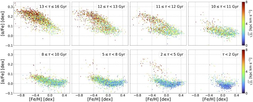
Chrono-chemokinematics of the Galactic disc                         2815
disc (e.g. Minchev et al. 2012; Grand et al. 2016; Kawata et al.              the asteroseismic age determined from  from the individual
2017).                                                                        radial-mode frequency from the Kepler light curve (Miglio et al.
   High-resolution numerical simulations also suggested several               2020).
thick and thin disc formation scenarios, including violent gas-rich              Gaia DR2 provides astrometric information to obtain the position
mergers at high-redshift (e.g. Brook et al. 2004; Grand et al. 2018,          and proper motion for ∼ 1.3 billion stars with unprecedented
2020), accretion of high-[α/Fe] stars (Abadi et al. 2003; Kobayashi &         accuracy (Lindegren et al. 2018) as well as high-quality multiband
Nakasato 2011; Tissera, White & Scannapieco 2012), vertical heating           photometry for a large subset of these stars (Evans et al. 2018; Riello
from satellite merging events (e.g. Quinn, Hernquist & Fullagar 1993;         et al. 2018). For a selected type of stars with a G-band magnitude
Villalobos & Helmi 2008), and turbulence in clumpy high-redshift              between about 4 and 13 magnitudes, the mean line-of-sight velocities
gas-rich disc (Noguchi 1998; Bournaud, Elmegreen & Martig 2009;               measured with Gaia Radial Velocity Spectrometer (RVS), line-of-
Beraldo e Silva et al. 2020). The recent popular view is that the             sight velocities have also been provided in Gaia DR2 (Cropper et al.
thick disc formation precedes the thin disc formation and the earlier         2018; Sartoretti et al. 2018; Katz et al. 2019). We use the photometric

                                                                                                                                                          Downloaded from https://academic.oup.com/mnras/article/503/2/2814/6162622 by UCL, London user on 31 March 2021
disc was smaller and thicker, i.e. an inside-out and upside-down              data from Gaia DR2 for BINGO, and the parallax and proper motion
formation of the disc (e.g. Brook et al. 2004, 2006; Bird et al. 2013).       information to derive the kinematic properties for our sample of stars.
In Brook et al. (2012), the majority of the thick-disc stars form as gas         APOGEE is a spectroscopic survey in the near-infrared H-band
originating from a gas-rich merger at high-redshift settles into a disc       (15 200 Å−16 900 Å) with a high resolution of R ∼ 22 500,
at the end of the merger epoch. This early disc is kinematically hot          observing more than 200 000 stars (as of DR14) located primarily
and radially compact. Once the chaotic phase of the star formation of         in the disc and bulge of the Milky Way. In this work, we employ
the thick disc ends, the younger, lower [α/Fe] thin disc can gradually        the calibrated stellar parameters such as effective temperature and
grow in an inside-out fashion (e.g. Matteucci & Francois 1989) as gas         surface gravity as well as metal abundances obtained with the
is smoothly accreting to the central galaxy. As in Brook et al. (2012),       APOGEE Stellar Parameters and Chemical Abundances Pipeline
Noguchi (2018), and Grand et al. (2018) suggested that chemical               (ASCAP; Garcı́a Pérez et al. 2016) in the APOGEE DR14 survey
evolution proceeds at different rates in the inner and outer disc,            (Abolfathi et al. 2018). In addition, we use the 2MASS J, H, K
resulting in more chemically evolved stars in the inner regions. Radial       photometry and their associated uncertainties (Skrutskie et al. 2006)
migration can bring the thick disc stars formed in the inner disc to          reported in the APOGEE DR14 catalogue.
the outer disc at redshift z ∼ 0, so that we can observe the thick
disc stars at the solar neighbourhood (Brook et al. 2012; Minchev,
Chiappini & Martig 2013).                                                     2.1 BINGO
   The Gaia mission (DR2; Gaia Collaboration 2018) is providing               Machine Learning has revolutionized the way we perform data
information to obtain the accurate position and motion for more               analysis tasks in Astronomy, which has grown into a big data field
than a billion stars in the Milky Way. The APOKASC-2 catalogue                with the emergence of large surveys such as SDSS and Gaia. Neural
(Pinsonneault et al. 2018), comprised of 6676 evolved stars in the            networks are Machine Learning methods that can, in principle, model
APOGEE DR14 survey observed by the Kepler mission (Borucki                    any smooth map between high-dimensional input data to a set of
et al. 2010), provides the best asteroseismology information to infer         desirable outputs. Depending on their architecture, neural networks
the age for giant stars, which is crucial for Galactic archaeology.           can consist of one or more fully connected layers, each with a
In this paper, we use a state-of-the-art machine learning method, a           number of neurons that essentially take the input and transform
Bayesian neural network, trained on the APOKASC-2 data, to obtain             it through linear activation functions to an output of interest (also
reliable relative stellar age estimates for 17 305 carefully selected         known as feed-forward artificial neural networks). In supervised
disc stars in the APOGEE data. We use the age, chemistry, and                 learning, which BINGO uses, the parameters of the neural network,
kinematical information to examine the formation history of the               e.g. weights that define the connection between neurons, are trained
Galactic disc by comparing our results with what is expected from             and optimized to best reproduce the training set where the input and
the formation scenarios of the thick and thin disc suggested by the           output are known. Then, the trained neural network can be applied
recent numerical simulations described above.                                 to the data whose output is unknown with much less computational
   This paper is organized as follows. Section 2 describes the                cost than training.
Bayesian Machine Learning framework, called BINGO (Bayesian                      In Bayesian Inference, the power of Bayes’ Law is that it allows
INference for Galactic archaeOlogy), that we employ in the current            us to relate the probability of a model given the data to a quantity that
analysis. We discuss here how the biases in the training data set affect      is easier to understand, namely the probability we would observe the
the performance of the neural network model and our approach to               data given the model and any background information, I, i.e.
minimize the bias in the subsequent inferences. In Section 3, we
present the results after applying BINGO to carefully selected stars          p(model|data, I ) ∝ p(data|model, I )p(model|I ),                    (1)
in the APOGEE survey. A brief discussion of our results is given in           where p(model|data, I) is the posterior probability, p(data|model, I) is
Section 4. Finally, a summary of our findings is given in Section 5.          the likelihood, and p(model|I) is the prior. The posterior encompasses
                                                                              our state of knowledge about a model given that we gather new data
2 METHOD                                                                      through the likelihood. Following equation (1), Bayes’ Law can be
                                                                              applied to a neural network to come up with a probability distribution
In this paper, we introduce BINGO that is a Bayesian Machine                  over its model parameters1 and construct a Bayesian Neural Network
Learning framework to obtain stellar ages of evolved stars us-                as done in the pioneering work of Das & Sanders (2018) and Sanders
ing photometric information from the second data release of the               & Das (2018). This powerful synergy between Bayesian Inference
European Space Agency’s (ESA) Gaia mission (Gaia DR2; Gaia                    and Machine Learning allows us to naturally introduce uncertainty
Collaboration 2018) and the stellar parameter information from the
fourteenth data release of the SDSS-IV APOGEE-2 (Majewski et al.
2017). BINGO consists of a Bayesian neural network trained using              1 https://twiecki.io/blog/2016/07/05/bayesian-deep-learning/

                                                                                                                    MNRAS 503, 2814–2824 (2021)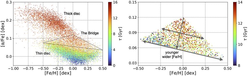
2816          I. Ciucă et al.
                                                                                         assumptions used to derive the asteroseismic ages that we are using
                                                                                         are given as R11 in table 1 of Miglio et al. (2020). We select only
                                                                                         red clump stars (RC) with masses higher than 1.8 M and the red
                                                                                         giant branch (RGB) stars, for which the relative asteroseismic ages
                                                                                         are reliable. To construct our base training set, we use only stars
                                                                                         with high signal-to-noise (SNR) APOGEE spectra (SNR > 100),
                                                                                         which leaves us with 2915 stars. We then use the APOGEE stellar
                                                                                         parameters and photometry data, Teff , log g, [α/M], [M/H],2 [C/Fe],
                                                                                         [N/Fe], G, BP, RP, J, H, and K as the input features in BINGO to
                                                                                         map them to the common logarithm of the asteroseismic age, log(τ ),
                                                                                         referred to as the target.
                                                                                            Because the original data come from a limited Kepler field data, our

                                                                                                                                                                      Downloaded from https://academic.oup.com/mnras/article/503/2/2814/6162622 by UCL, London user on 31 March 2021
                                                                                         original training set has a known dependence of age and metallicity
                                                                                         on the distance (which affects photometry). Also, there are not many
                                                                                         young or old stars in our selected RGB and RC data. To correct
                                                                                         for the distance dependence, we randomly displace the distance of
                                                                                         stars between 0 and 10 kpc and then adjust the apparent magnitude
Figure 1. Schematics of a Bayesian neural network with two hidden layers.                of the stars depending on the difference between the new distance
Each connection between neurons has an associated weight and the neurons                 and the original distance. We do not change the extinction upon
in the hidden and output layers have an associated bias. The connection                  displacing the distance also to erase the dependence of extinction on
between neurons i in the input layer and j in the first hidden layer has the             the distance. We refer to this technique as distance shuffling.
associated weight w i, j and the neuron j has a bias b1, j . Each weight and bias           Our training set contains a smaller number of young (age  12 Gyr) stars, and this imbalance becomes
of the neuron j, and shows the transformation applied to the input data xi in            more apparent when using log (τ ) as our target variable for BINGO.
the first hidden layer of the network, namely xi → f( i (w i, j xi ) + b1, j ), where
                                                                                         During training, the model learns to reproduce the target variable
f is the activation function. We use a rectified linear unit (ReLU) activation
                                                                                         only for a majority of intermediate age stars, which biases the
function in our analysis.
                                                                                         prediction towards the intermediate age irrespective of their true
                                                                                         age, and consequently leads to overpredicting the age of younger
into our machine learning approach, i.e. we can get an estimate of                       stars and underpredicting the age of the very old stars, an effect also
how confident our neural network is of its predictions.                                  known as regression dilution. To minimize the effect of this bias
   BINGO’s architecture consists of two fully connected layers with                      and balance our training set, we effectively oversample the fewer
16 neurons each (Fig. 1). We use the probabilistic programming                           young stars and very old stars to balance the number of stars at
framework PYMC3 (Salvatier, Wiecki & Fonnesbeck 2015) and its                            different log (τ ). To this end, we first examine the distribution of
Magic Inference Button, the No-U-Turn-Sampler (NUTS) as the                              our original training set in log (τ ). We then use a Kernel Density
MCMC sampler. We use a Gaussian prior of N (0, σ ) for the weights                       Estimator (KDE) to approximate the distribution in log (τ ), and
and bias parameters in the neural network, which effectively acts as                     for each star, we find its probability under the KDE, which we
L2 regularization. It is possible to optimize σ of the Gaussian prior,                   refer to as prob. We then compute the inverse probability and
but it is computationally too expensive. Therefore, we adopt σ =                         round it the nearest integer, N = [1/prob]. Following the distance
1 for simplicity. We use four chains that allow us to diagnose our                       shuffling procedure described above, we randomly distance-shuffle
samples and make sure the samples returned from the NUTS sampler                         each star N times. This approach leads to some of the stars in the
are drawn from the target distribution. Once we have a posterior                         original data set to be sampled more than once. Since their distances
distribution over the neural network parameters, we can then compute                     and hence their apparent magnitude are different, these ‘artificial’
a distribution over the network outputs by marginalizing over the                        stars become members of an augmented training set. Since we are
network parameters. We note that this Bayesian Neural Network                            using data augmentation, which is an established machine learning
scheme assumes that all the input features, such as the stellar param-                   technique, we refer to our approach as age data augmentation.
eters, are independent, and cannot take into account the covariance                      The final training set has 4673 stars after performing the age data
between the inputs. It is also worth noting that the neural network                      augmentation technique on the training set data (80 per cent of
model depicted in Fig. 1 is not identifiable (Pourzanjani, Jiang &                       the original data). Note that the data augmentation can reduce the
Petzold 2017). Hence, the naive MCMC sampling of the network                             uncertainties in our predictions, because we artificially increase the
parameters suffers from the unidentifiability of the parameters. Still,                  number of data points. Therefore, our uncertainties do not statistically
we have confirmed that the posterior distribution of the target age                      reflect the uncertainty in the measurement of the stellar age. In this
prediction from the four different chains are consistent with each                       paper, however, our priority is to mitigate regression dilution with
other. Therefore, we are confident that our age prediction, especially                   this simple data augmentation technique. This is another caveat of
the mean of the prediction used in this paper, does not suffer severely                  BINGO in addition to the assumed independence of the input features
from unidentifiability. These known challenges for Bayesian Neural                       and the unidentifiability discussed above. In this paper, as described
Networks remain caveats of BINGO, upon which we hope to improve                          later, we use the uncertainties only as the metric of confidence of
in a future study.

                                                                                         2 InAPOGEE DR14, α-elements comprise of O, Mg, Si, S, Ca, and Ti. We
2.2 Building an effective training set
                                                                                         used the ASPCAP measurements of [α/M] and [M/H] as a proxy for [α/Fe]
In this study, we employ a training set created from the APOKASC-2                       and [Fe/H], respectively. Correspondingly, we use the labels of [α/Fe] and
data set with our derived asteroseismic age (Miglio et al. 2020). The                    [Fe/H] to refer to [α/M] and [M/H].

MNRAS 503, 2814–2824 (2021)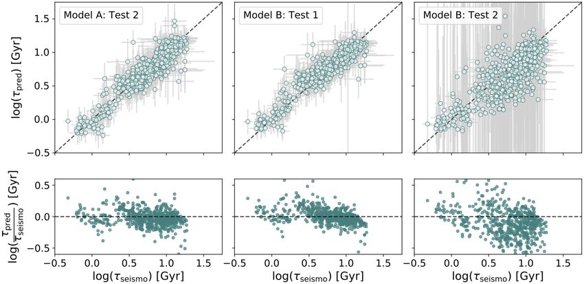
Chrono-chemokinematics of the Galactic disc                        2817
                                                                                       in the output label, i.e. log (τ ). We therefore use Model A in this
                                                                                       paper.

                                                                                       2.3 RGB and high mass RC selection
                                                                                       Our training set consists of the specific population of RC stars with
                                                                                       a mass higher than 1.8 M and RGB stars in the limited Kepler field.
                                                                                       When we apply our trained model to the rest of APOGEE data, we
                                                                                       select only the same population as the population of the training
                                                                                       data. Hence, we train a three-layer artificial neural network on the
                                                                                       original APOKASC-2 data to classify RC stars with a mass higher
                                                                                       than 1.8 M and RGB stars. For this classification task, we train the

                                                                                                                                                                  Downloaded from https://academic.oup.com/mnras/article/503/2/2814/6162622 by UCL, London user on 31 March 2021
Figure 2. Comparison between observed (target) logarithmic age of stars,
                                                                                       model using KERAS and TENSORFLOW (Abadi et al. 2016), which
log (τ seismo ), derived with asteroseismology and the predicted log (τ pred ) by
                                                                                       is much less computationally expensive than training a Bayesian
BINGO. The panels show the results when applying the model trained with
the age data augmented training set with the distance shuffling (Model A)              Neural Network. The selection function of APOKASC-2 is not the
to the original test data (Test 1, see Section 2.2 for details). The light green       same as the rest of the APOGEE data. However, because we need
circles in the left-hand panel show the model prediction results against the           the stellar mass and the RC, RGB and AGB classification for the
observed target age. The standard deviation in the prediction and observation          training and validation data, we use the APOKASC-2 data for training
are shown as the grey lines. The right-hand panel shows the difference                 and validation. We have constructed a classification neural network
between prediction and target, which peaks at 0 with a standard deviation              to identify the RC stars with > 1.8 M and RGB stars using our
of 0.1 dex.                                                                            asteroseismic analysis of the APOKASC-2 data. We used the input
                                                                                       features of Teff , log g, [α/Fe], [Fe/H], [C/Fe], [N/Fe], G, BP, RP, J,
our prediction, and do not use the uncertainties for any quantitative                  H, and K, and 2948 positive, i.e. the high mass RC or RGB, and
discussion. Hence, the discussion of this paper is unlikely to be                      1918 negative stars are used for the training. Similar strategies are
affected by these issues. We postpone the resolution of these issues                   employed in Hawkins, Ting & Walter-Rix (2018) and Ting, Hawkins
to a future study.                                                                     & Rix (2018) to identify the RC stars.
   To evaluate the prediction accuracy of BINGO, we split our                             We then use the trained neural network model to classify stars
original data of 2915 stars into training (80 per cent, 2331 stars) and                in the APOGEE cross-matched with Gaia DR2 data set (Sanders &
testing (20 per cent, 583 stars) data. To demonstrate the importance                   Das 2018). We also limit our data to having APOGEE spectra with
of distance shuffling and age data augmentation, we consider two                       SNR > 100 and the K-band extinction smaller than 0.1 mag in the
different trained models: Model A trained on the age data augmented                    APOGEE catalogue, because all of our training data has the K-band
training set of 4673 stars with the distance shuffling and Model B                     extinction  5.0. We compute the
measurement (Miglio et al. 2020).                                                      distance using the Gaia parallax with the additional systematic bias
   Fig. 3 presents the predictions from Model A on Test 2 (left),                      of parallax of 54 μas (Schönrich, McMillan & Eyer 2019), and select
from Model B on Test 1 (middle), and Test 2 (right). There is little                   the stars in the limited volume of 7 < R < 9 kpc and z < 2 kpc, where
difference between Model A on Test 1 (see Fig. 2 )and Model A on                       we assume the solar position at the Galactocentric distance of 8 kpc
Test 2. This means that BINGO Model A can recover the age well                         and the vertical height of the Sun from the disc plane of 0.025 kpc.
in application data which have no distance dependence in age or                        We obtain kinematic properties using GALPY (Bovy 2015). We have
metallicity. The middle panel of Fig. 2 shows that Model B trained                     confirmed that our derived age and kinematics are consistent with
on the original data set without the age data augmentation leads to a                  Sanders & Das (2018), except for the difference in the absolute age
systematic overprediction for the age of stars with the asteroseismic                  scales, because we use a different asteroseismic age scale for our
age of log (τ seismo ) < 0.5 dex and underprediction of the age for                    training set (Miglio et al. 2020). As a result, we obtain 17 305 stars,
stars with log (τ seismo ) > 1.0 dex. This is because Model B is trained               which are used in the following sections.
mainly to reproduce the overwhelming number of stars with 0.5
< log (τ seismo ) < 1.0 dex and suffers from the regression dilution
                                                                                       3 R E S U LT S
effect mentioned above. The right-hand panel of Fig. 3 shows the
age prediction of Model B on Test 2, which shows much worse                            In this section, we explore the relations between stellar age, chemistry
recovery of the asteroseismic ages with large uncertainties. This                      and orbital properties for our sample of stars. Reliable relative age
is because Model B has learned the dependence of the age and                           estimates for a large number of stars obtained with BINGO enable us
metallicity on the distance in the original training set. These results                to find that the inner and outer discs follow a different formation and
demonstrate why it is important to erase the distance dependence                       chemical evolution pathway. Our results provide further evidence for
in the training set and keep the balance of the number of sample                       an upside-down, inside-out formation of the Galactic disc.

                                                                                                                           MNRAS 503, 2814–2824 (2021)
2818         I. Ciucă et al.

                                                                                                                                                                      Downloaded from https://academic.oup.com/mnras/article/503/2/2814/6162622 by UCL, London user on 31 March 2021
Figure 3. Predictions versus the target asteroseismic age in log (τ ). Left-hand panel shows the result from a model trained on the age data augmented training
set with the distance shuffling (Model A) and applied to the distance shuffled test set (Test 2). The middle and right-hand panels show the predictions for a
model trained on the original data (Model B) applied to the original (Test 1) and distance shuffled test data (Test 2), respectively. The standard deviation in the
prediction and asteroseismic age are shown as the grey lines. Model A predictions for Test 2 perform better than Model B prediction for Test 1. The model
trained on the original data and applied to the distance shuffle data, i.e. Model B prediction for Test 2, performs considerably worse as Model B has learned the
distance dependence of age and metallicity, which is erased in Test 2.

Figure 4. [α/Fe] as a function of age coloured by metallicity, [Fe/H]. The          Figure 5. [Fe/H] as a function of age coloured by [α/Fe]. The younger
high-[α/Fe] population ([α/Fe]>0.1 dex) is older and more metal-poor.               population is more metal-rich than its older counterpart. Stars more metal-
                                                                                    poor than −0.5 dex are considerably old.

3.1 The chrono-chemical map of disc stars
                                                                                    agreement with Silva Aguirre et al. (2018). However, considering
We first investigate the evolution of α-abundances, [α/Fe], and                     the uncertainties of the age, this relationship is considered to be tight
metallicity, [Fe/H], with age, τ . Fig. 4 shows the enhancement in                  (Haywood et al. 2013; Snaith et al. 2015). A striking feature of Fig. 4
[α/Fe] as a function of age coloured by metallicity. The deficiency                 is the young, low metallicity, high-α stars, also seen in Chiappini
of stars with age ∼ 1.5 Gyr arises because we select the RC stars                   et al. (2015), Martig et al. (2015), and Silva Aguirre et al. (2018). We
with mass > 1.8 M and there are considerably fewer RGB stars                       discuss the origin of this population in more detail in Section 3.3.
with ages younger than 3 Gyr. The high-[α/Fe] ‘sequence’ separates                     Fig. 5 shows the age–metallicity relationship coloured with [α/Fe].
clearly from the low-[α/Fe] ‘sequence’ in the age-[α/Fe] space at                   While the old, high-[α/Fe] stars exhibit a clear trend of decreasing
[α/Fe] ∼ 0.1 dex, where there seems to be a population gap extending                [Fe/H] with age, the younger, low-[α/Fe] disc shows a flat age-
approximately 0.02 dex. The majority of the high-[α/Fe] stars ([α/Fe]               [Fe/H] relation up to ∼ 11 Gyr. For stars with [Fe/H] >−0.5 dex, our
> 0.1 dex) are generally older and more metal-poor than the low-                    results are qualitatively similar to those from previous studies, such as
[α/Fe] population. [α/Fe] rapidly decreases with decreasing age up                  Casagrande et al. (2011), Silva Aguirre et al. (2018), and Mackereth
to ∼ 10 Gyr. The age-[α/Fe] relationship also appears to be broader                 et al. (2019). For the metal-poor and high [α/Fe] population, the
in [α/Fe] at a fixed age for the high-[α/Fe] population, in qualitative             tight trend observed between age and metallicity is consistent with

MNRAS 503, 2814–2824 (2021)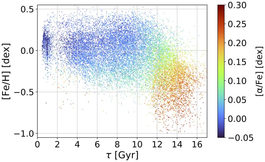
Chrono-chemokinematics of the Galactic disc                                   2819

                                                                                                                                                                          Downloaded from https://academic.oup.com/mnras/article/503/2/2814/6162622 by UCL, London user on 31 March 2021
Figure 6. The distribution of [α/Fe] and [Fe/H] coloured by age for our sample of stars. We refer to the old high- and young low-[α/Fe] populations as the thick
and thin disc, respectively, as highlighted in the left-hand panel. The dotted triangle region in the left-hand panel is referred to as the Bridge, and is a transition
region between the thick (high-α sequence with [α/Fe]  0.1 dex) and thin disc (low-[α/Fe] sequence). An age gradient is apparent, as indicated by the near
vertical downward arrow, in a close-up of the Bridge region, shown in the right-hand panel, and the range of [Fe/H] becomes wider, as indicated by the two near
horizontal arrows for the younger stars in the Bridge region.

Bensby et al. (2005) and Haywood et al. (2013), who analysed dwarf                    of age and vertical action Jz . The general trend is that Jz is decreasing
stars and used the isochrone age.                                                     with age, with the older population being significantly hotter than the
   In Fig. 6, we examine the distribution in [α/Fe] and [Fe/H]                        younger population. As also inferred from Fig. 6, Fig. 7 clearly shows
coloured by age for the stars in our sample. Classically, this diagram                that the Bridge region starts appearing at age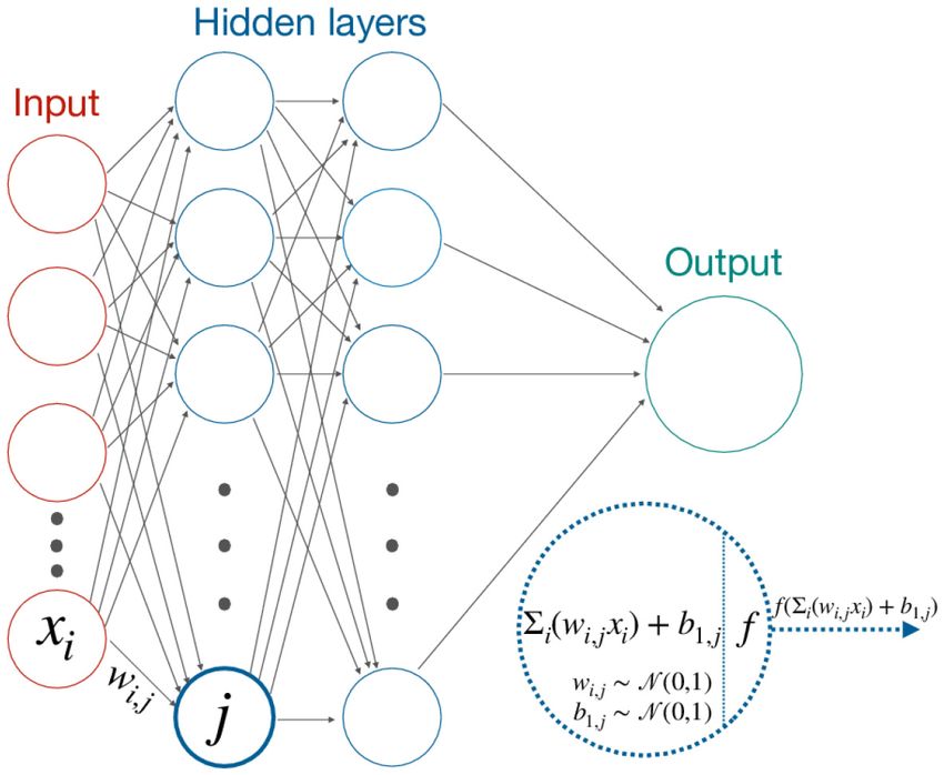
2820 I. Ciucă et al.
Downloaded from https://academic.oup.com/mnras/article/503/2/2814/6162622 by UCL, London user on 31 March 2021
√
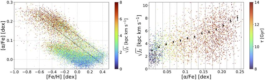
Figure 7. The distribution of [α/Fe] and [Fe/H] coloured by the square root of the vertical action, Jz , for the samples of stars within eight different age bins.
The top four panels show [Fe/H]–[α/Fe] relationship for the older stars (10 < τ < 16 Gyr), and the lower four panels present those for the younger stars (τ <
10 Gyr). There is a kinematically hot population of young high-[α/Fe] stars seen in the lower panels.
√
Figure 8. Left-hand panel: the distribution of [α/Fe] and [Fe/H] coloured by the square root of the vertical action, Jz . The ridge selection in the left-hand
√
panel represents the highest metallicity track in the [Fe/H]–[α/Fe] space. Right-hand panel: the [α/Fe]- Jz relationship coloured by age in the ridge region
highlighted in the left-hand panel. We overlay the scale heights (black dots) and uncertainties (error bars) measured by fitting an isothermal profile to the
distribution of p(Jz ) in 13 bins in [α/Fe]. Analysis of the high-[Fe/H] ridge shows that Jz smoothly decreases with [α/Fe] and age.
Figure 9. The distribution in [α/Fe] versus [Fe/H] (left-hand panel), [Fe/H] versus age (middle panel), and [α/Fe] versus age (right-hand panel) coloured by
mean orbital radius, Rm . The ‘inner’, ‘local’, and ‘outer’ arrows indicate the schematic chemical evolution paths at the inner (Rm ∼6 kpc), local, i.e. solar
radius (Rm ∼8 kpc), and outer discs (Rm ∼10 kpc), respectively. The metal-poor, outer disc stars follow a different chemical evolution pathway than the inner
disc. These evolutionary paths are shown to describe qualitative trends of the chemical evolution at the different radii of the Galactic disc, and are not meant to
indicate the chemical evolution paths quantitatively.
MNRAS 503, 2814–2824 (2021)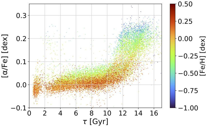
Chrono-chemokinematics of the Galactic disc                               2821

                                                                                                                                                                       Downloaded from https://academic.oup.com/mnras/article/503/2/2814/6162622 by UCL, London user on 31 March 2021
                                                              √                                                                                    √
Figure 10. The distribution in Rm (left-hand panel) and Jz (right-hand               Figure 11. The distribution in Rm (left-hand panel) and Jz (right-hand
panel) for old (log (τ [Gyr]) > 1.0) stars with [α/Fe] >0.12 dex, shown in red,      panel) for stars with [α/Fe] >0.12 dex, shown in red, and young (0.2 <
and young (log (τ [Gyr]) < 0.8) stars with [α/Fe] >0.12 dex, shown in blue.          log (τ [Gyr]) < 0.5) stars with [α/Fe]  9 kpc). Hence, we                   [α/Fe] stars that appear young originated from the old high-[α/Fe]
consider that the low-[Fe/H], low-[α/Fe] stars formed at the outer                   thick disc stars.
disc and their star formation started when the disc grew large enough                   By combining the age information with the chemistry and kine-
to develop a wide range of [Fe/H], i.e. the metallicity gradient, at                 matics, we can constrain the origin of the kinematically hot young
the end of the transition period of the Bridge after the old thick disc              high-[α/Fe] population. Our results are in agreement with Silva
formation. As a result, the star formation and chemical evolution                    Aguirre et al. (2018), and Miglio et al. (2020), who also found similar
path should be different from the inner disc, and the stars in the outer             kinematical properties between young high-[α/Fe] stars and young
disc do not originate in the thick disc formation phase.                             low-[α/Fe]. We confirmed their results with a larger number of 69
    This different path of the disc formation in the inner disc and                  young high-[α/Fe] stars. Miglio et al. (2020) also found a higher
the outer disc is schematically described with the arrows in Fig. 9.                 fraction of young (overmassive) high-[α/Fe] population in RC stars
The arrows highlighted with ‘inner’, ‘local’, and ‘outer’ indicate the               than RGB stars, and discussed that this is consistent with a scenario
chemical evolution paths at the inner, local, i.e. solar radius, and                 that these young [α/Fe] stars are the merged binaries, because more
outer discs, respectively, inferred from our data. The middle panel                  binaries are expected to have undergone an interaction around the tip
shows that low-[Fe/H] stars start forming later than the inner disc and              of RGB than fainter RGB.
are systematically younger than the thick disc, which is formed only
in the inner disc. The right-hand panel shows that the lower-[Fe/H]
outer thin disc stars are higher [α/Fe]. This is seen as a positive [α/Fe]           4 I M P L I C AT I O N S F O R T H E D I S C F O R M AT I O N
radial gradient in the thin disc (e.g. Hayden et al. 2015).                          A N D E VO L U T I O N
                                                                                     Our results suggest a formation scenario for the Galactic disc that
                                                                                     involves distinct star formation and chemical evolution pathways of
3.3 The young high-[α/Fe] stars
                                                                                     the inner and outer discs. In the inner disc, the thick disc forms
The lower panels of Fig. 7, consisting of stars younger than 10 Gyr,                 early on from chemically well-mixed and turbulent gas, which can
reveal the existence of a population of kinematically hot, high-[α/Fe]               be, for example, associated with gas-rich mergers (e.g. Brook et al.
stars. To understand their origin, we look at the distribution in Rm                 2004), cold gas flow accretion (e.g. Kereš et al. 2005; Dekel &
and Jz between stars with [α/Fe] >0.12 dex and old (log (τ [Gyr]) >                  Birnboim 2006; Brooks et al. 2009; Ceverino, Dekel & Bournaud
1.0) and stars with [α/Fe] >0.12 dex and young (log (τ [Gyr]) < 0.8).                2010; Fernández, Joung & Putman 2012) or, most likely, a complex
As shown in Fig. 10, the two groups of stars overlap significantly in                interplay of both (e.g. Grand et al. 2018, 2020). Such a thick disc
both Rm and Jz distributions. Fig. 11, where we compared between                     formation scenario can explain the clear and tight age-[α/Fe] (Fig. 4),
[α/Fe] >0.12 dex stars and young stars (0.2 < log (τ [Gyr]) < 0.5)                   age-[Fe/H] (Fig. 5), and [Fe/H]–[α/Fe] sequence (Fig. 6) for the old
having [α/Fe]
2822 I. Ciucă et al.
by the ‘inner’ pathway in Fig. 9. There is no distinct epoch of Consequently, the stars currently around the solar radius follow the
thick and thin disc formation, as seen in the ridge region of Fig. 8. so-called two-infall model (Grisoni et al. 2017; Spitoni et al. 2019),
Instead, the thicker to thinner disc transition happens in a smooth although the high-[α/Fe] populations are formed in the inner disc
manner as stars continue to form with lower Jz from the dense and brought to the solar neighbourhood likely by radial migration.
cold gas continuously present at this radius (Brook et al. 2012; On the other hand, if we could select only the stars formed locally,
Grand et al. 2018). The smooth transition between the thick and thin the star formation starts at a later epoch from lower metallicity gas,
discs in the inner region naturally arises in multizone semi-analytical when the star-forming disc becomes as large as the solar radius. In
chemo-dynamical evolution models (e.g. Schönrich & Binney 2009; other words, the stars started forming locally around the solar radius
Schönrich & McMillan 2017), where stars keep forming from the from the second infall of gas, whose metallicity is lower, because of
left-over gas of the high-[α/Fe] sequence. the dilution with the metal-poor gas accreted from the halo (Calura
A smooth transition between the formation of the thick and thin & Menci 2009; Spitoni et al. 2019; Buck 2020). The scenario is
discs in the inner region is also suggested as the ‘centralized starburst also consistent with what is suggested by Snaith et al. (2015) and
Downloaded from https://academic.oup.com/mnras/article/503/2/2814/6162622 by UCL, London user on 31 March 2021
pathway’ in Grand et al. (2018). Using the high-resolution AURIGA Haywood et al. (2016, 2019). In fact, by private communication with
cosmological simulations of the Milky Way (Grand et al. 2017), Misha Haywood after the submission of the first version of this paper,
Grand et al. (2018) propose the ‘centralized starburst pathway’ model we realized that our schematic view in Fig. 9 is consistent with fig. 6
that can explain the single sequence of the [α/Fe]–[Fe/H] distribution of Haywood et al. (2019), except that they considered that the outer
in the inner disc seen in the APOGEE data of Hayden et al. (2015; low-[α/Fe] stars formed earlier than the inner low-[α/Fe] stars.
see also Palla et al. 2020). In their model, a major gas-rich merger
and cold gas accretion at an early epoch initiate a short period of
5 S U M M A RY
intense star formation in the inner region during which the thick disc
forms with higher [α/Fe]. Once Type Ia SNe become significant in In this paper, we determine precise relative stellar age estimates for
chemical enrichment after the peak of star formation in ∼ 1 Gyr 17 305 evolved stars in the APOGEE DR14 survey using a Bayesian
time-scale, more metal-rich low-[α/Fe] thin disc stars continuously Neural Network trained on the APOKASC-2 asteroseismic data set.
form from the left-over less turbulent gas in the inner disc. As a To minimize the bias in our age inference, we erase the distance
result, there is no gap in the formation of the thick and thin disc dependence of metallicity and age in our training set by randomly
and a single sequence of [α/Fe]–[Fe/H] is expected in the inner disc. displacing the distance of the stars. We also augment the data set
Then, we can observe such inner disc stars in our data due to radial by oversampling young and very old stars, to obtain a balanced
migration (e.g. Brook et al. 2012; Minchev et al. 2013; Kawata et al. training data and minimize the effect of regression dilution. Using
2018; Renaud et al. 2020), which brings them within 7 < R < 9 kpc. the chemo-kinematical information, we separate the Galactic disc
Our results also suggest that the star formation and chemical into three components, the thick and thin discs and the Bridge in
evolution in the outer disc starts after the thick disc phase. When the [Fe/H]–[α/Fe] distribution. The thick disc population is older
the thick-disc like, gas-rich merger- and/or cold accretion-dominant, and higher-[α/Fe] ([α/Fe] 0.12) than the thin disc. We argue that
turbulent star formation ends, the Galactic halo may have grown the Bridge population connects the thick disc and thin disc phases
enough for the hot gas accretion mode to become dominant (Brooks smoothly, rather than being part of the traditional thick disc. We also
et al. 2009; Noguchi 2018). Then, the violent cold gas accretion find an unusual population of young and high-[α/Fe] stars. However,
stops, and the gas disc can grow in an inside-out fashion, as fresh we found that their kinematic properties are similar to the old high-
low [Fe/H] gas is accreted smoothly from the hot halo gas. The disc [α/Fe] stars, which suggests that their origin must be the same as the
rapidly grows large enough to develop a negative metallicity gradient old high-[α/Fe] stars. They are identified as young stars likely due
as seen in the Bridge region of Fig. 6, unlike for the turbulent small to the merger of binary stars which decreased [C/N] and led to the
thick disc phase, where the metals are well mixed, and no metallicity predicted young ages.
gradient can develop. Hence, the metal-poor outer disc developed To further investigate whether or not there is a smooth transition
after the thick disc formation, as indicated by the arrow of the ‘outer’ between the formation of the thick and thin disc in the inner region,
disc chemical evolution pathway in Fig. 9. we select a high-metallicity ridge region in the [Fe/H]-[α/Fe] plane
The Bridge region in Fig. 6 shows that the range of [Fe/H] that follows a continuously increasing [Fe/H] and decreasing [α/Fe]
becomes wider for the younger stars, as indicated by the arrows sequence. We examined the variation of Jz with [α/Fe] and age and
in the left-hand panel of Fig. 6. We consider that the Bridge region concluded that, while there seems to be a hint of a sudden decrease in
is where the thin disc formation begins, and the disc is developing Jz around [α/Fe] ∼ 0.12 dex, Jz smoothly decreases with [α/Fe] and
a metallicity gradient with younger stars forming with a broader also with age. We find that the oldest stars are kinematically hotter
range of [Fe/H]. Radial migration brings stars formed in the inner and enhanced in α-abundances than the younger stars. We found that
disc and outer disc to the solar neighbourhood, which is where the the high-metallicity ridge is dominated by the stars from the inner
stars in our samples lie (but see also Vincenzo & Kobayashi 2020; disc and traces the continuous chemical evolution of the inner disc,
Khoperskov et al. 2021, who claim that radial migration is not very R < 6 kpc. The formation of the thick disc is expected to happen
efficient). As a result, we can observe the mixed chemical distribution in a compact disc, i.e. only in the inner disc, and a turbulent period
from pathways in the inner and outer discs (Schönrich & Binney of intense chemical mixing leads to the relatively tight sequence
2009). The high metallicity ridge highlighted in Fig. 8 represents in the distribution of [α/Fe] and [Fe/H] for the old stars. From our
the chemical evolution of the inner disc. The low-[Fe/H] and low- results, we infer that the inner disc continuously forms stars from the
[α/Fe] stars came from the outer disc. As a result, we observe the two left-over gas after the thick disc formation phase and the subsequent
sequences of the high- and low-[α/Fe] stars in our sample (Brook accreting gas, and develop high-[Fe/H] and low-[α/Fe] stars.
et al. 2012; Grand et al. 2018). This is consistent with what is seen in We also found that the outer low-[Fe/H] and low-[α/Fe] stars are
the previous observational studies (e.g. Hayden et al. 2017; Feuillet significantly younger than the inner high-[α/Fe] ([α/Fe] 0.12 dex)
et al. 2019). Our results provide more robust trends with more reliably stars. We argue that the outer metal-poor disc stars form after the end
measured relative ages. of cold-mode dominated violent thick disc formation phase. This
MNRAS 503, 2814–2824 (2021)Chrono-chemokinematics of the Galactic disc 2823
likely corresponds to the transition from the cold to hot mode of operations grant ST/R00689X/1. DiRAC is part of the National e-
the gas accretion due to the halo mass growth (Grand et al. 2018; Infrastructure.
Noguchi 2018).
In light of these results, we argue that the inner and outer discs of
DATA AVA I L A B I L I T Y
the Milky Way follow different chemical evolution pathways. After
the violent thick disc formation phase ends, the thin disc formation The data underlying this article will be shared on reasonable request
starts with a smaller disc which is as small as the thick disc, and then to the corresponding author.
the thin disc grows in an inside-out fashion. As the disc is growing
with a supply of accreting low-[Fe/H] gas, metallicity gradients
naturally arise, with the outer disc being more metal-poor than the REFERENCES
inner disc. We found that the Bridge region shows a broader range Abadi M. et al., 2016, preprint (arXiv:1603.04467)
of [Fe/H] with decreasing age, and suggest that the Bridge region is Abadi M. G., Navarro J. F., Steinmetz M., Eke V. R., 2003, ApJ, 597, 21
Downloaded from https://academic.oup.com/mnras/article/503/2/2814/6162622 by UCL, London user on 31 March 2021
where the thin disc formation begins, and the disc is developing a Abolfathi B. et al., 2018, ApJS, 235, 42
metallicity gradient. Anders F. et al., 2014, A&A, 564, A115
The recent work of Grand et al. (2020) suggested that the last Anders F., Chiappini C., Santiago B. X., Matijevič G., Queiroz A. B.,
significant merger of Gaia–Enceladus–Sausage (GES; Brook et al. Steinmetz M., Guiglion G., 2018, A&A, 619, A125
Bekki K., Tsujimoto T., 2011, ApJ, 738, 4
2003; Belokurov et al. 2018; Haywood et al. 2018; Helmi et al.
Belokurov V., Erkal D., Evans N. W., Koposov S. E., Deason A. J., 2018,
2018) was a gas-rich merger that was essential in forming the thick MNRAS, 478, 611
disc. This picture is also consistent with what we found in this paper Bensby T., Feltzing S., Lundström I., Ilyin I., 2005, A&A, 433, 185
because this gas-rich merger can induce a violent starburst in the Bensby T., Alves-Brito A., Oey M. S., Yong D., Meléndez J., 2011, ApJ, 735,
inner disc due to the dissipation of the gas during the merger. If L46
the GES merger was the last significant merger, then the thin disc Beraldo e Silva L., Debattista V. P., Khachaturyants T., Nidever D., 2020,
phase could start after the GES merger settled. If this scenario is MNRAS, 492, 4716
true, the end of the GES merger could correspond to the high-[α/Fe] Binney J., 2010, MNRAS, 401, 2318
tip ([α/Fe] ∼ 0.12 dex, [Fe/H] ∼ 0.0 dex) of the Bridge region of Binney J., McMillan P., 2011, MNRAS, 413, 1889
Fig. 6. After that, the thin disc grew inside-out from the smooth Bird J. C., Kazantzidis S., Weinberg D. H., Guedes J., Callegari S., Mayer L.,
Madau P., 2013, ApJ, 773, 43
accretion of the low metallicity gas from the hot halo gas. Although
Borucki W. J. et al., 2010, Science, 327, 977
this is admittedly pure speculation, we could test this hypothesis if we Bournaud F., Elmegreen B. G., Martig M., 2009, ApJ, 707, L1
measured the relative difference in ages between the GES, the GES Bovy J., 2015, ApJS, 216, 29
merger remnants (e.g. Chaplin et al. 2020; Montalbán et al. 2020), Bovy J., Rix H.-W., Liu C., Hogg D. W., Beers T. C., Lee Y. S., 2012, ApJ,
high-[α/Fe] thick disc and the Bridge. Measuring the age difference 753, 148
of stars precisely represents the holy grail of Galactic archaeology, Brooks A. M., Governato F., Quinn T., Brook C. B., Wadsley J., 2009, ApJ,
as it allows us to improve our understanding of stellar evolution and 694, 396
probe deeper into the formation and evolution history of the Milky Brook C. B., Kawata D., Gibson B. K., Flynn C., 2003, ApJ, 585, L125
Way. Brook C. B., Kawata D., Gibson B. K., Freeman K. C., 2004, ApJ, 612, 894
Brook C. B., Kawata D., Martel H., Gibson B. K., Bailin J., 2006, ApJ, 639,
126
AC K N OW L E D G E M E N T S Brook C. B. et al., 2012, MNRAS, 426, 690
Buck T., 2020, MNRAS, 491, 5435
We thank our anonymous referee for their helpful comments to Calura F., Menci N., 2009, MNRAS, 400, 1347
improve the manuscript. IC and DK acknowledge the support of Casagrande L., Schönrich R., Asplund M., Cassisi S., Ramı́rez I., Meléndez
the UK’s Science and Technology Facilities Council (STFC Grant J., Bensby T., Feltzing S., 2011, A&A, 530, A138
ST/N000811/1 and ST/S000216/1). IC is also grateful for the STFC Ceverino D., Dekel A., Bournaud F., 2010, MNRAS, 404, 2151
Doctoral Training Partnerships Grant (ST/N504488/1). IC thanks Chaplin W. J. et al., 2020, Nat. Astron., 4, 382
the LSSTC Data Science Fellowship Program, where their time Cheng J. Y. et al., 2012, ApJ, 752, 51
as a Fellow has benefited this work. AM acknowledges support Chiappini C., Matteucci F., Gratton R., 1997, ApJ, 477, 765
Chiappini C., Matteucci F., Romano D., 2001, ApJ, 554, 1044
from the ERC Consolidator Grant funding scheme (project AS-
Chiappini C. et al., 2015, A&A, 576, L12
TEROCHRONOMETRY, grant agreement number 772293). GRD
Cropper M. et al., 2018, A&A, 616, A5
has received funding from the European Research Council (ERC) Das P., Sanders J. L., 2018, MNRAS, 484, 294
under the European Union’s Horizon 2020 research and innovation Dekel A., Birnboim Y., 2006, MNRAS, 368, 2
programme (CartographY GA. 804752). This work has made use of Delgado Mena E. et al., 2019, A&A, 624, A78
data from the European Space Agency (ESA) mission Gaia (https: Evans D. W. et al., 2018, A&A, 616, A4
//www.cosmos.esa.int/gaia), processed by the Gaia Data Processing Fernández X., Joung M. R., Putman M. E., 2012, ApJ, 749, 181
and Analysis Consortium (DPAC, https://www.cosmos.esa.int/web Feuillet D. K., Frankel N., Lind K., Frinchaboy P. M., Garcı́a-Hernández D.
/gaia/dpac/consortium). Funding for the DPAC has been provided A., Lane R. R., Nitschelm C., Roman-Lopes A., 2019, MNRAS, 489,
by national institutions, in particular, the institutions participating in 1742
Fuhrmann K., 1998, A&A, 338, 161
the Gaia Multilateral Agreement. This work was inspired from our
Gaia Collaboration, 2018, A&A, 616, A11
numerical simulation studies used the UCL facility Grace and the
Garcı́a Pérez A. E. et al., 2016, AJ, 151, 144
Cambridge Service for Data Driven Discovery (CSD3), part of which Gilmore G., Reid N., 1983, MNRAS, 202, 1025
is operated by the University of Cambridge Research Computing on Grand R. J. J., Springel V., Gómez F. A., Marinacci F., Pakmor R., Campbell
behalf of the STFC DiRAC HPC Facility (www.dirac.ac.uk). The D. J. R., Jenkins A., 2016, MNRAS, 459, 199
DiRAC component of CSD3 was funded by BEIS capital funding Grand R. J. J. et al., 2017, MNRAS, 467, 179
via STFC capital grants ST/P002307/1 and ST/R002452/1 and STFC Grand R. J. J. et al., 2018, MNRAS, 474, 3629
MNRAS 503, 2814–2824 (2021)2824 I. Ciucă et al.
Grand R. J. J. et al., 2020, MNRAS, 497, 1603 Montalbán J. et al., 2020, preprint (arXiv:2006.01783)
Grisoni V. et al., 2017, MNRAS, 472, 3637 Nidever D. L. et al., 2014, ApJ, 796, 38
Hawkins K., Ting Y.-S., Walter-Rix H., 2018, ApJ, 853, 20 Noguchi M., 1998, Nature, 392, 253
Hayden M. R. et al., 2015, ApJ, 808, 132 Noguchi M., 2018, Nature, 559, 585
Hayden M. R., Recio-Blanco A., de Laverny P., Mikolaitis S., Worley C. C., Palla M., Matteucci F., Spitoni E., Vincenzo F., Grisoni V., 2020, MNRAS,
2017, A&A, 608, L1 498, 1710
Haywood M., Di Matteo P., Lehnert M. D., Katz D., Gómez A., 2013, A&A, Pinsonneault M. H. et al., 2018, ApJS, 239, 32
560, A109 Pourzanjani A. A., Jiang R. M., Petzold L. R., 2017, Proceedings of NIPS
Haywood M., Lehnert M. D., Di Matteo P., Snaith O., Schultheis M., Katz Workshop on Bayesian Deep Learning
D., Gómez A., 2016, A&A, 589, A66 Prochaska J. X., Naumov S. O., Carney B. W., McWilliam A., Wolfe A. M.,
Haywood M., Di Matteo P., Lehnert M. D., Snaith O., Khoperskov S., Gómez 2000, AJ, 120, 2513
A., 2018, ApJ, 863, 113 Queiroz A. B. A. et al., 2020, A&A, 638, A76
Haywood M., Snaith O., Lehnert M. D., Di Matteo P., Khoperskov S., 2019, Quinn P. J., Hernquist L., Fullagar D. P., 1993, ApJ, 403, 74
Downloaded from https://academic.oup.com/mnras/article/503/2/2814/6162622 by UCL, London user on 31 March 2021
A&A, 625, A105 Renaud F., Agertz O., Read J. I., Ryde N., Andersson E. P., Bensby T., Rey
Helmi A., Babusiaux C., Koppelman H. H., Massari D., Veljanoski J., Brown M. P., Feuillet D. K., 2020, preprint (arXiv:2006.06011)
A. G. A., 2018, Nature, 563, 85–88 Riello M. et al., 2018, A&A, 616, A3
Izzard R. G., Halabi G. M., 2018, preprint (arXiv:1808.06883) Roškar R., Debattista V. P., Loebman S. R., 2013, MNRAS, 433, 976
Jofré P. et al., 2016, A&A, 595, A60 Salvatier J., Wiecki T., Fonnesbeck C., 2015, preprint (arXiv:1507.08050)
Katz D. et al., 2019, A&A, 622, A205 Sanders J. L., Das P., 2018, MNRAS, 481, 4093
Kawata D., Grand R. J. J., Gibson B. K., Casagrande L., Hunt J. A. S., Brook Sartoretti P. et al., 2018, A&A, 616, A6
C. B., 2017, MNRAS, 464, 702 Schönrich R., Binney J., 2009, MNRAS, 399, 1145
Kawata D. et al., 2018, MNRAS, 473, 867 Schönrich R., McMillan P. J., 2017, MNRAS, 467, 1154
Kereš D., Katz N., Weinberg D. H., Davé R., 2005, MNRAS, 363, 2 Schönrich R., McMillan P., Eyer L., 2019, MNRAS, 487, 3568
Khoperskov S., Haywood M., Snaith O., Di Matteo P., Lehnert M., Vasiliev Silva Aguirre V. et al., 2018, MNRAS, 475, 5487
E., Naroenkov S., Berczik P., 2021, MNRAS, 501, 5176 Skrutskie M. F. et al., 2006, AJ, 131, 1163
Kobayashi C., Nakasato N., 2011, ApJ, 729, 16 Snaith O., Haywood M., Di Matteo P., Lehnert M. D., Combes F., Katz D.,
Lindegren L. et al., 2018, A&A, 616, A2 Gómez A., 2015, A&A, 578, A87
Loebman S. R., Roškar R., Debattista V. P., Ivezić, Ž., Quinn T. R., Wadsley Spitoni E., Silva Aguirre V., Matteucci F., Calura F., Grisoni V., 2019, A&A,
J., 2011, ApJ, 737, 8 623, A60
Mackereth J. T. et al., 2019, MNRAS, 489, 176–195 Ting Y.-S., Rix H.-W., 2019, ApJ, 878, 21
Majewski S. R. et al., 2017, AJ, 154, 94 Ting Y.-S., Hawkins K., Rix H.-W., 2018, ApJ, 858, L7
Martig M. et al., 2015, MNRAS, 451, 2230 Tissera P. B., White S. D. M., Scannapieco C., 2012, MNRAS, 420, 255
Matteucci F., Francois P., 1989, MNRAS, 239, 885 Villalobos Á., Helmi A., 2008, MNRAS, 391, 1806
Miglio A. et al., 2021, A&A, 645, A85 Vincenzo F., Kobayashi C., 2020, MNRAS, 496, 80
Minchev I., Famaey B., Quillen A. C., Dehnen W., Martig M., Siebert A.,
2012, A&A, 548, A127
Minchev I., Chiappini C., Martig M., 2013, A&A, 558, A9
This paper has been typeset from a TEX/LATEX file prepared by the author.
MNRAS 503, 2814–2824 (2021)You can also read