Evaluation of VEGETATION and PROBA-V Phenology Using PhenoCam and Eddy Covariance Data - MDPI
←
→
Page content transcription
If your browser does not render page correctly, please read the page content below
remote sensing
Article
Evaluation of VEGETATION and PROBA-V
Phenology Using PhenoCam and Eddy
Covariance Data
Kevin Bórnez 1,2, *, Andrew D. Richardson 3,4 , Aleixandre Verger 1,2 , Adrià Descals 1,2                and
Josep Peñuelas 1,2
 1    CREAF, Cerdanyola del Vallès, 08193 Bellaterra, Catalonia, Spain; verger@creaf.uab.cat (A.V.);
      a.descals@creaf.uab.cat (A.D.); Josep.Penuelas@uab.cat (J.P.)
 2    CSIC, Global Ecology Unit CREAF-CSIC-UAB, 08193 Bellaterra, Catalonia, Spain
 3    Center for Ecosystem Science and Society, Northern Arizona University, Flagstaff, AZ 86011, USA;
      Andrew.Richardson@nau.edu
 4    School of Informatics, Computing and Cyber Systems, Northern Arizona University, Flagstaff,
      AZ 86011, USA
 *    Correspondence: k.bornez@creaf.uab.cat

 Received: 17 August 2020; Accepted: 16 September 2020; Published: 19 September 2020

 Abstract: High-quality retrieval of land surface phenology (LSP) is increasingly important for
 understanding the effects of climate change on ecosystem function and biosphere–atmosphere
 interactions. We analyzed four state-of-the-art phenology methods: threshold, logistic-function,
 moving-average and first derivative based approaches, and retrieved LSP in the North Hemisphere
 for the period 1999–2017 from Copernicus Global Land Service (CGLS) SPOT-VEGETATION and
 PROBA-V leaf area index (LAI) 1 km V2.0 time series. We validated the LSP estimates with near-surface
 PhenoCam and eddy covariance FLUXNET data over 80 sites of deciduous forests. Results showed
 a strong correlation (R2 > 0.7) between the satellite LSP and ground-based observations from both
 PhenoCam and FLUXNET for the timing of the start (SoS) and R2 > 0.5 for the end of season (EoS). The
 threshold-based method performed the best with a root mean square error of ~9 d with PhenoCam
 and ~7 d with FLUXNET for the timing of SoS (30th percentile of the annual amplitude), and ~12 d
 and ~10 d, respectively, for the timing of EoS (40th percentile).

 Keywords: Land-surface phenology; SPOT-VEGETATION; PROBA-V; leaf area index; PhenoCam;
 FLUXNET

1. Introduction
     The study of vegetation phenology and its patterns on a global scale have become more important
since the late twentieth century for analyzing the effects of climate change [1,2]. Remote sensing is a
useful tool for characterizing land surface phenology (LSP) [3] and global changes of vegetation [4–6].
De Beurs et al. [7] analyzed a broad range of statistical methods designed to extract phenological
metrics from satellite time series based on threshold percentiles [8–10], moving averages [11], first
derivatives [12,13], smoothing functions [14] and fitted models [15].
     Most literature on LSP has focused on the use of time series of vegetation indices mainly derived
from MODIS data [6,16,17]. In previous studies, we showed the added value of using Copernicus
Global Land Service (CGLS) leaf area index (LAI) time series derived from VEGETATION and
PROBA-V data [10,18]. Bórnez et al. [18] found that the phenological metrics extracted from the CGLS
LAI Version 2 (V2) time series agreed best with the available human-based ground observations of
phenological transition dates for deciduous broadleaf forest in Europe (PEP727) and United States

Remote Sens. 2020, 12, 3077; doi:10.3390/rs12183077                         www.mdpi.com/journal/remotesensing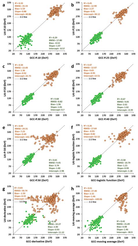
Remote Sens. 2020, 12, 3077                                                                          2 of 17

of America (USA-NPN) as compared to other biophysical variables and NDVI vegetation index or
previous version V1 of the CGLS products.
      Validating LSP is challenging due, in part, to the differences in the definition of satellite metrics
and ground phenophases [13,19]. Volunteer observers have traditionally collected data for the timing
of specific phenophases of individual plants [20]. Human observations of phenology, however,
are not uniform and may induce uncertainties, despite efforts to establish protocols for monitoring
phenophases [21–23].
      Near-surface remote sensing using conventional red-green-blue (RGB) digital cameras provides an
alternative to human observations to monitor vegetation phenology [24–28] because of their low cost,
ease of set up and capacity to collect detailed spectral information at high temporal frequencies [29]
of individual plants, species or canopies [30] across broad spatial scales [31–33]. PhenoCam [34] is a
network of digital cameras that currently includes >600 site-years of imagery, with high-quality and
high temporal resolution providing data of vegetation phenology. Deciduous broadleaved forests
(68 sites) are the dominant vegetation type within the PhenoCam Network [35], and the focus of this
study. A growing number of studies have compared transition dates derived from the PhenoCam time
series of green chromatic coordinates (GCC) with satellite phenological metrics derived mainly from
MODIS data [29,36–38].
      Continuous flux measurements from eddy covariance technique also started to be used as a
new perspective for estimating LSP at the landscape level [5,39–43]. The flux measurements sites are
organized as a confederation of regional networks around the world, called FLUXNET [44]. Until the
last updated of February 2020, the most recent dataset produces was the FLUXNET2015 dataset [44]
which includes data from 212 sites [45].
      In this study, we build on our previous work [18] and take advantage now of PhenoCam and
FLUXNET capability of continuous monitoring of vegetation seasonal growth at very high temporal
resolution, with data every 30 minutes [26,46–49]. This allows a more robust and accurate comparison
with LSP derived from satellite time series avoiding problems related to the differences in the definition
of phenology metrics. We evaluated four methods for estimating phenology: the threshold method
based on percentiles [10], the derivative method [12], the autoregressive moving-average method [11]
and the logistic-function method [50]. These methods were applied both to satellite CGLS LAI V2 time
series and ground observations from PhenoCam GCC and eddy covariance flux towers over deciduous
forests to assess the accuracy of LSP retrievals.

2. Materials and Methods

2.1. Study Area
      The study was conducted over the North Hemisphere in pixels classified as deciduous forests or
mixed vegetation according to the annual C3S Global Land Cover for the year 2018 [51]. The validation
was done over PhenoCam sites distributed across North America and one in Europe, and FLUXNET
towers sites both in North America and Europe and one in Japan. We selected only deciduous forests
sites with at least 2 years of available observations. This resulted in 64 sites from PhenoCam, and 16
towers of FLUXNET covering a broad range of latitudes (30–60◦ N) and elevations (1-1870 m a.s.l.)
(Figure 1 and Table S1).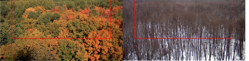
Remote Sens. 2020, 12, 3077 3 of 17
Remote Sens. 2020, 12, 3077 3 of 17
Figure 1.
Figure 1. Locations
Locationsof the selected
of the PhenoCam
selected sites (red)
PhenoCam sitesand FLUXNET
(red) towers (black)
and FLUXNET over(black)
towers deciduous
over
forests. forests.
deciduous
2.2.
2.2.Satellite
SatelliteData:
Data: CGLS
CGLS LAI
LAI
We
Weused
usedCopernicus
Copernicus land
land surface
surface products (CGLS
(CGLS LAI LAI V2)
V2) derived
derivedfromfromSPOT-VEGETATION
SPOT-VEGETATION
(1999–2013)
(1999–2013)and andPROBA-V
PROBA-V (2014-2017)
(2014-2017)data. The The
data. spatial resolution
spatial is 1 kmisand
resolution the and
1 km temporal frequency
the temporal
isfrequency
10 d [52]. is 10 d [52].
The
The algorithm
algorithm forfor LAI
LAI V2V2 product
product [53,54]
[53,54] capitalizes on on the
the development
development and and validation
validationofof
already
alreadyexisting
existingproducts
products (CYCLOPES
(CYCLOPES version 3.1 and and MODIS
MODIS collection
collection55products)
products)and
andthe
theuse
useofof
neuralnetworks
neural networks[55].
[55]. The
The inputs
inputs of the neural networks
networks are are daily
dailytop
topofofthe
thecanopy
canopyreflectances
reflectancesfrom
from
VEGETATION and PROBA-V in the red, near-infrared and shortwave infrared spectral bands andand
VEGETATION and PROBA-V in the red, near-infrared and shortwave infrared spectral bands the
the and
sun sun and
view view geometry.
geometry. A multi-step
A multi-step procedurefor
procedure forfiltering,
filtering,temporal
temporal smoothing,
smoothing, gap-filling
gap-fillingand
and
compositingisisthen
compositing thenapplied
appliedtoto the
the daily
daily estimates
estimates to generate the final 10 d products
products [53].
[53].
2.3.
2.3.PhenoCam
PhenoCamData
Data
We
Weused
usedPhenoCam
PhenoCamDataset
DatasetV1.0
V1.0[34,56].
[34,56]. It provides digital
digital images
images every
every3030min.
min.InIneach
eachimage,
image,
aa“region
“regionofofinterest”
interest”was
was defined
definedmanually
manuallybased
basedon on
thethe
dominant
dominant vegetation
vegetation typetype
in the
in camera field
the camera
offield
viewof[35]
view [35] (Figure
(Figure 2). The2).size
Theofsize
the of thetypically
ROI ROI typically
rangesranges
from ~50from to~50 to m
~500 2
~500 m [34,35].
[34,35].
2 The
The green
green chromatic
chromatic coordinate
coordinate (GCC) (GCC) index
index [35] was[35] was calculated
calculated from
from the redthe(R),red (R), (G)
green greenand(G) and(B)
blue blue (B)
digital
digital numbers
numbers (DN) as: (DN) as:
GDN
ீே
Gcc =ܿܿܩRDN
ൌ + GDN (1)(1)
ோ ାீ ା+ BDN
ே ே ே
We
Weused
usedthe
the90th percentile G
90thpercentile CC value and 1 d high quality
GCC quality composites
composites toto avoid
avoidnoise
noisefrom
from
variations
variationsin
inmeteorological,
meteorological, atmospheric
atmospheric or illumination conditions [57].
illumination conditions [57]. We
Wemanually
manuallyfiltered
filteredthe
the
poor-qualityGG
poor-quality CC
CCobservations
observations and
and then
thengap-filled
gap-filledthe missing
the data
missing with
data a
withlocally
a weighted
locally scatter-plot
weighted scatter-
smoother (lowess)-based
plot smoother filter filter
(lowess)-based [35]. [35].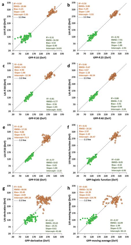
Remote Sens. 2020, 12, 3077                                                                                       4 of 17
 Remote Sens. 2020, 12, 3077                                                                                       4 of 17

       Figure2.2. PhenoCam
      Figure      PhenoCamimages
                             imagescaptured
                                    capturedin  in(A)
                                                   (A)spring,
                                                       spring,(B)
                                                                (B)summer,
                                                                    summer,(C)(C)autumn
                                                                                  autumnandand(D)
                                                                                               (D)winter
                                                                                                     winterover
                                                                                                            overthe
                                                                                                                 the
       NEON.D05.UNDE.DP1.00033 site
      NEON.D05.UNDE.DP1.00033         site (46.23 ◦
                                            (46.23°N,
                                                    N, 89.54 ◦
                                                       89.54°W).   The red
                                                               W). The red rectangle
                                                                            rectangle indicates
                                                                                       indicates the
                                                                                                  theborders
                                                                                                      bordersof
                                                                                                              ofthe
                                                                                                                 the
       selectedregion
      selected  regionof
                       ofinterest.
                          interest.

2.4.
 2.4. FLUXNET
      FLUXNET Data
              Data
      We
      We used    FLUXNET 2015
          used FLUXNET       2015collection
                                    collectionofofgross
                                                     gross   primary
                                                         primary       production
                                                                   production        (GPP)
                                                                                 (GPP) flux flux
                                                                                             data data
                                                                                                   over over   16
                                                                                                         16 forest
forest tower   sites (Figure 1) for the  period   2003–2014    (110 site-years)  [44]. We used   the
 tower sites (Figure 1) for the period 2003–2014 (110 site-years) [44]. We used the daily GPP (g C m-2daily  GPP
(g     −2 d−1 ) derived from half-hourly eddy covariance flux measurements using the night time based
   C mderived
 d-1)            from half-hourly eddy covariance flux measurements using the night time based
approach
 approach[58,59].
            [58,59].We
                     Wesmoothed
                         smoothedthe theseries
                                         seriesofofthe
                                                    thedaily
                                                        dailyGPP
                                                              GPPbybyusing
                                                                       usinga aSavitzky–Golay
                                                                                Savitzky–Golay filter based
                                                                                                  filter     onon
                                                                                                         based  a
second  degree
 a second  degreepolynomial
                    polynomialand  a 30-day
                                 and         smoothing
                                      a 30-day   smoothing window
                                                              window [60–62].
                                                                        [60–62].
2.5. Methods for Estimating Vegetation Phenology
 2.5. Methods for Estimating Vegetation Phenology
      We tested four methods for estimating phenology (Table 1 and Figure 3, [18]) from satellite
      We tested four methods for estimating phenology (Table 1 and Figure 3, [18]) from satellite
(CGLS LAI time series) and ground-based data (PhenoCam GCC, FLUXNEX GPP) (e.g., Figure S2
 (CGLS LAI time series) and ground-based data (PhenoCam GCC, FLUXNEX GPP) (e.g., Figure S2 in
in Supplementary Materials). The phenological metrics are the timing of the start of the growing
 Supplementary Materials). The phenological metrics are the timing of the start of the growing season
season (SoS), the end of the growing season (EoS) and the length of the growing season (LoS). LoS was
 (SoS), the end of the growing season (EoS) and the length of the growing season (LoS). LoS was
estimated as the length of time between the EoS and the SoS. The CGLS LAI 10 d time series were
 estimated as the length of time between the EoS and the SoS. The CGLS LAI 10 d time series were
linearly interpolated at daily steps before phenological retrieval.
 linearly interpolated at daily steps before phenological retrieval.

       Table 1. Description of the evaluated methods for the extraction of phenology metrics.

      Method.       Reference                      Principles and parameters
   Threshold based Verger et al. SoS is defined as the first day of the year (DoY) when the
    on percentiles [10]          vegetation variable exceeds a particular threshold. EoS is
                                 defined as the DoY when an index descends below a threshold.
                                 We established dynamic thresholds per pixel based on a
                                 percentile (10th, 25th, 30th, 40th and 50th) of the annual
                                 amplitude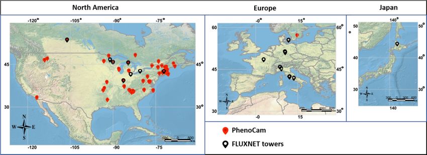
Remote Sens. 2020, 12, 3077                                                                                                                                                   5 of 17

                                             Table 1. Description of the evaluated methods for the extraction of phenology metrics.

                          Method.                                Reference                                           Principles and Parameters
                                                                                       SoS is defined as the first day of the year (DoY) when the vegetation variable exceeds
                                                                                       a particular threshold. EoS is defined as the DoY when an index descends below a
            Threshold based on percentiles             Verger et al. [10]
                                                                                       threshold. We established dynamic thresholds per pixel based on a percentile (10th,
                                                                                       25th, 30th, 40th and 50th) of the annual amplitude
                                                                                       SoS is defined as the DoY with the first local maximum rate of change in the curvature
                     Logistic function                 Zhang et al. [50]               of a logistic function fitted to the time series. EoS is defined as the DoY with the first
                                                                                       local minimum rate of change in the curvature
                                                                                       SoS is defined as the DoY of the maximum increase (maximum first derivative) in the
                      First derivative                 Tateishi and Ebata. [12]
                                                                                       curve. EoS is defined as the DoY of the maximum decrease in the curve
                                                                                       A moving average is first computed at a given time lag (we tested 10–50 d and
            Autoregressive moving average              Reed et al. [11]                selected a 30 d time lag). SoS and EoS are then defined as the DoY when the
                                                                                       moving-average curves cross the original time series of the vegetation index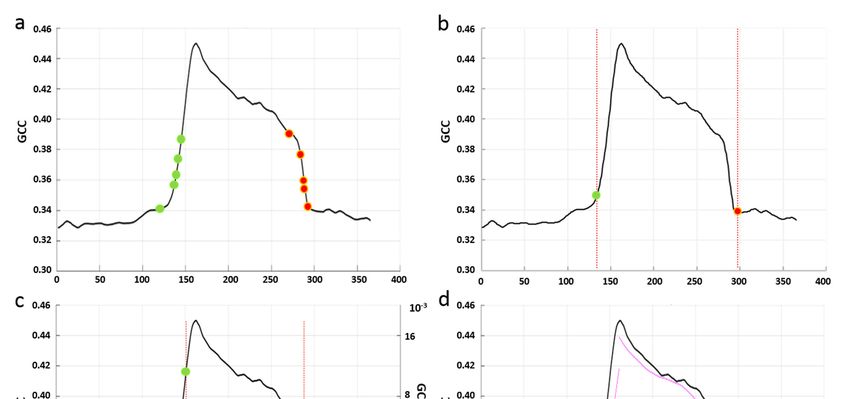
[12]              maximum decrease in the curve
  Autoregressive            Reed et al. A moving average is first computed at a given time lag (we
  moving average            [11]        tested 10–50 d and selected a 30 d time lag). SoS and EoS are then
                                        defined as the DoY when the moving-average curves cross the
Remote Sens. 2020, 12, 3077
                                        original time series of the vegetation index                   6 of 17

     Figure
     Figure 3.    Illustrationof
              3. Illustration   ofthe
                                   thethreshold
                                       threshold(a), (a),logistic-function
                                                           logistic-function    (b),
                                                                             (b),     derivative
                                                                                   derivative   (c) (c)
                                                                                                     andand   moving-average
                                                                                                          moving-average   (d)
     (d) phenological
     phenological         extraction
                       extraction     methods
                                   methods        applied
                                               applied            PhenoCamGG
                                                            to toPhenoCam             time series of Acadia site (44.37◦ N,
                                                                                CCCCtime series of Acadia site (44.37ºN,
     68.26 ◦ W) for 2014. The green and red points correspond to SoS and EoS, respectively. The different
     68.26ºW)    for 2014. The green and red points correspond to SoS and EoS, respectively. The different
     points
     points in    panel aa correspond
              in panel      correspond to to the
                                              the percentiles
                                                    percentiles 10th,
                                                                    10th, 25th,
                                                                           25th, 30th,
                                                                                  30th, 40th
                                                                                          40th and
                                                                                                and50th.50th. The
                                                                                                              The purple
                                                                                                                  purple line
                                                                                                                         line
     corresponds     to the first derivative  in c, and    to the  moving   average
     corresponds to the first derivative in c, and to the moving average in d.         in d.

2.6. Validation Approach
2.6. Validation Approach
      The LSP derived from VEGETATION and PROBA-V LAI V2 time series was compared with
      The LSP derived from VEGETATION and PROBA-V LAI V2 time series was compared with the
the LSP estimates using ground data from PhenoCam and FLUXNET when the same phenological
LSP estimates using ground data from PhenoCam and FLUXNET when the same phenological
extraction method was applied (Section 3.1). The statistical metrics used for assessing the performance
extraction method was applied (Section 3.1). The statistical metrics used for assessing the
are the root mean square error (RMSE), the mean error (bias); the coefficient of determination (R2 ),
performance are the root mean square error (RMSE), the mean error (bias); the coefficient of
slope and intercept of the Reduced Major Axis regression (RMA). Further the spatial patterns and
determination (R2), slope and intercept of the Reduced Major Axis regression (RMA). Further the
latitudinal gradients of LSP estimates were assessed in Section 3.2. We used RStudio for the statistical
spatial patterns and latitudinal gradients of LSP estimates were assessed in Section 3.2. We used
analysis, Google Earth Engine (GEE, https://earthengine.google.org) for the retrieval of LSP over the
RStudio for the statistical analysis, Google Earth Engine (GEE, https://earthengine.google.org) for the
North Hemisphere, and ESRI ArcGIS 10.5 and gvSIG-desktop-2.3.1 for the graphs and maps.

3. Results

3.1. Comparison of Satellite and Ground Phenologies
     The coefficient of determination, R2 , between the satellite- and ground-based estimates from
PhenoCam and FLUXNET phenology ranges from 0.01 to 0.81 (p < 0.001) (Table 2). The threshold-based
method provided the best performances. The 30th percentile of annual amplitude was the best
threshold for the SoS (RMSE < 9 d, bias < 2 d and R2 = 0.74 with p < 0.001 for CGLS LAI V2 estimates
compared to PhenoCam; and RMSE < 7 d, bias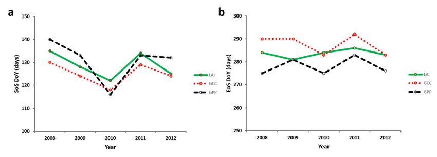
Remote Sens. 2020, 12, 3077 7 of 17
Table 2. Statistics of the comparison between the SOS and EOS dates retrieved using the LAI, GCC,
and GPP estimates for the four methods: thresholds, logistic function, derivative and moving average.
* indicates significant correlations at p < 0.05; **, significant correlations at p < 0.001. The bold type
highlights the best method. Evaluation over the 64 PhenoCam sites (356 samples (sites × years)) and
16 FLUXNET towers (110 samples (sites × years)) over deciduous forests in the North Hemisphere
(Figure 1).
Metric Validation Method RMSE BIAS R2 Slope Intercept
SoS PhenoCam Threshold (10th percentile) 17.80 −0.53 0.29 1.07 −8.57
Threshold (25th percentile) 9.92 1.29 0.61 ** 1.02 −8.57
Threshold (30th percentile) 8.82 1.96 0.74 ** 1.01 0.7
Threshold (40th percentile) 9.05 2.61 0.67 ** 1.02 −0.39
Threshold (50th percentile) 9.45 3.74 0.65 ** 1.00 2.98
Logistic function 10.79 1.21 0.58 ** 0.99 1.18
Derivative 19.27 2.40 0.18 0.93 11.12
Moving average 15.49 0.48 0.42 * 1.24 −30.9
SoS FLUXNET Threshold (10th percentile) 16.50 3.54 0.31 0.90 14.03
Threshold (25th percentile) 7.91 −2.08 0.7 ** 1.00 −2.91
Threshold (30th percentile) 6.77 −3.56 0.81 ** 1.03 −8.02
Threshold (40th percentile) 7.21 −3.91 0.80 ** 0.99 −3.24
Threshold (50th percentile) 8.42 −5.65 0.77 ** 1.04 −11.8
Logistic function 8.05 -0.42 0.69 ** 0.94 6.06
Derivative 23.63 −14.31 0.19 0.61 41.66
Moving average 16.09 1.99 0.37 * 0.79 30.13
EoS PhenoCam Threshold (10th percentile) 15.33 5.59 0.33 * 0.88 40.86
Threshold (25th percentile) 12.90 2.27 0.45 * 0.91 28.12
Threshold (30th percentile) 13.49 1.36 0.39 * 0.92 22.75
Threshold (40th percentile) 12.07 0.65 0.51 ** 0.95 13.51
Threshold (50th percentile) 29.31 7.23 0.09 0.49 142.16
Logistic function 17.64 −0.93 0.26 0.82 52.52
Derivative 50.74 −1.50 0.03 0.33 179.59
Moving average 27.40 2.15 0.01 1.46 −140.06
EoS FLUXNET Threshold (10th percentile) 10.84 6.25 0.5 ** 1.00 5.93
Threshold (25th percentile) 9.80 5.29 0.55 ** 1.04 −5.93
Threshold (30th percentile) 9.99 4.90 0.44 * 1.06 -12.38
Threshold (40th percentile) 9.67 4.67 0.53 ** 1.18 −46.54
Threshold (50th percentile) 17.39 9.88 0.18 0.76 71.9
Logistic function 10.26 2.97 0.41 * 1.10 −26.47
Derivative 48.06 32.40 0.01 −0.09 289.18
Moving average 31.50 −14.30 0.04 0.53 114.78
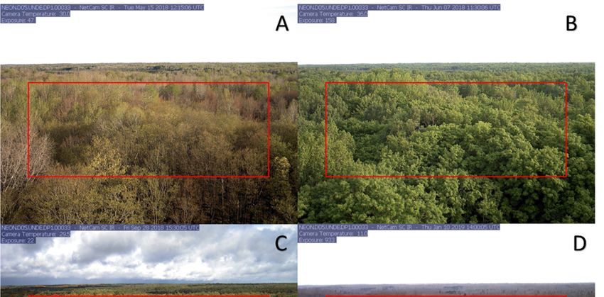
Figures 4 and 5 show the scatter plots of the comparison of satellite and ground-based SoS and
EoS retrievals for the four methods. The points were very close to the 1:1 line using the percentile and
logistic-function methods while the derivative and moving-average methods produced worse results
with more widely dispersed points, especially for the timing of EoS.
The satellite SoS (Figure 4, Figure 5 and Figure S1) retrieved with threshold and logistic-function
methods showed RMSE < 11 d and bias < 2 d compared to PhenoCam, and RMSE < 8 d and bias
< 4 d with FLUXNET (Table 2). Higher discrepancies for the SoS were found with the derivative
and moving-average methods: RMSE of 19 d and 15 d, and bias of 2 d and < 1 d, respectively using
PhenoCam estimates, and RMSE of 24 d and 16 d, and bias of –14 d and 2 d, respectively with FLUXNET
estimates (Table 2).
The EoS can be also robustly estimated using remote sensing observations (Figure 4, Figure 5 and
Figure S1) although we observed a degradation of performances for all the methods for the estimation
of the EoS as compared to the SoS: higher dispersion of points, higher RMSE and lower correlation for
EoS (Table 2). The EoS estimates from satellite time series of LAI agreed the best with GCC and GPP
derived phenology metrics using the threshold method followed by the logistic function: RMSE of
12 d and 18 d, respectively, and biases < 1 d compared to PhenoCam, and RMSE of 10 d and bias < 5 d
with FLUXNET (Table 2). The performance highly decreased for the derivative and moving average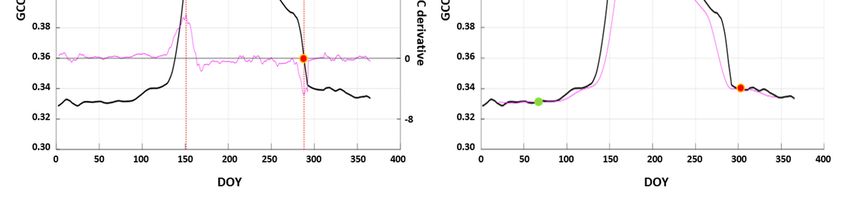
Remote Sens. 2020, 12, 3077                                                                                                  8 of 17

methods with RMSE of 50 d and 27 d, respectively, compared to PhenoCam, and RMSE of 48 d and 31
d with FLUXNET, and no significant correlation (R2 < 0.2) (Table 2).
   Remote Sens. 2020, 12, 3077                                                         8 of 17

      Figure       Scatterplots
               4. 4.
          Figure      Scatterplotsfor
                                    forSoS
                                        SoS (in
                                             (in green)
                                                 green) and    EoS (in
                                                          and EoS     (in orange)
                                                                          orange)estimated
                                                                                     estimatedfromfrom  CGLS
                                                                                                      CGLS   LAILAI
                                                                                                                  V2 V2
                                                                                                                      andand
      PhenoCam      GCC    time series by  the threshold   (10th (a),  25th (b), 30th  (c), 40th (d) and
          PhenoCam GCC time series by the threshold (10th (a), 25th (b), 30th (c), 40th (d) and 50th (e) 50th (e) percentiles
      of LAI  amplitude),
          percentiles  of LAIlogistic-function    (f), derivative
                               amplitude), logistic-function    (f),(g) and moving-average
                                                                     derivative                   (h) methods.
                                                                                 (g) and moving-average          Statistics of
                                                                                                            (h) methods.
      the Statistics
          comparison      are presented   in Table   2.
                     of the comparison are presented in Table 2.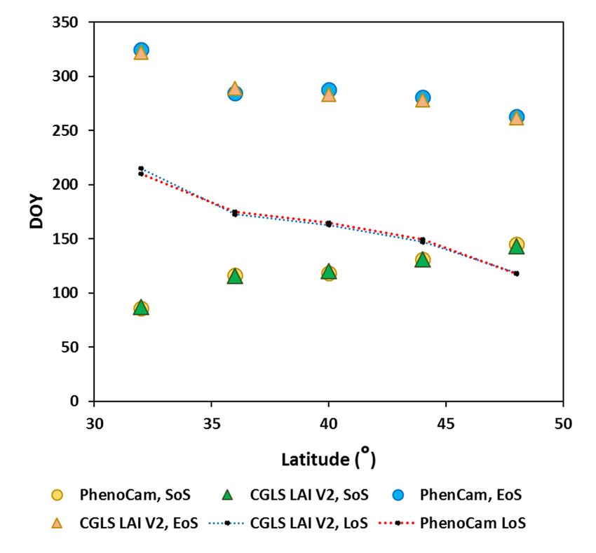
Remote Sens. 2020, 12, 3077                                                                                                   9 of 17
Remote Sens. 2020, 12, 3077                                                                                                9 of 17

     Figure
      Figure 5.
              5. Scatterplots
                  Scatterplotsfor
                                forSoS
                                     SoS(in(ingreen)
                                                green)andandEoS
                                                              EoS(in(inorange)
                                                                         orange)estimated
                                                                                    estimated from
                                                                                                 fromCGLS
                                                                                                       CGLS  LAI  V2V2
                                                                                                                LAI    andand
     FLUXNET
      FLUXNETGPP  GPPtime
                       timeseries
                             seriesby
                                    bythe
                                        thethreshold
                                             threshold(10th
                                                         (10th(a),
                                                                (a),25th
                                                                     25th(b), 30th
                                                                           (b),    (c),
                                                                                30th    40th
                                                                                     (c),    (d)(d)
                                                                                          40th   and  50th
                                                                                                    and    (e)(e)
                                                                                                        50th   percentiles
                                                                                                                  percentiles
     of
      of LAI
         LAI amplitude,
             amplitude, logistic-function      (f), derivative
                          logistic-function (f),    derivative (g)
                                                                (g) and
                                                                     andmoving-average
                                                                          moving-average(h)   (h)methods.
                                                                                                   methods.Statistics
                                                                                                              Statisticsofofthe
     the  comparison   are presented   in
      comparison are presented in Table 2.Table    2.
Remote Sens. 2020, 12, 3077 10 of 17
Remote Sens. 2020, 12, 3077 10 of 17
3.2. Latitudinal
Latitudinal Gradients
Gradients of
of Satellite
Satellite and Ground-Based Phenology
Figure S3 shows the spatial distribution of the GCLS LAI phenological estimates (SoS, EoS, and
LoS) from 2000 to 2017 over the North Hemisphere using the threshold method. The The length
length of the
vegetation cycles
cyclesregularly
regularly decreases from 220 days to 80 days when latitude
decreases from 220 days to 80 days when latitude increases from temperate increases from
temperate to boreal
to boreal regions. regions.
The The SoS
SoS ranges widelyranges
from widely from in
late march late march
the southintothe south to approximately
approximately mid-July in
mid-July
the north.inThethe SoS
north. The SoS earlier
is slightly is slightly earlier Europe
in central in central Europe
than than America
in North in North America for the
for the same same
latitude.
latitude. The EoS date ranges from early
The EoS date ranges from early August to December. August to December.
The latitudinal
latitudinal patterns
patternsofofthethetimings
timingsofofSoS SoS and
and EosEos derived
derived from
from CGLS
CGLS LAILAI V2 (Figure
V2 (Figure S3)
S3) and
and PhenoCam
PhenoCam GCCGCC over over deciduous
deciduous forestsforests 30◦ N30ºN
from from to 53◦toN53ºN in North
in North America
America showed showed
a verya good
very
good agreement
agreement with awith a gradual
gradual decrease
decrease in theinlength
the length of growing
of growing season
season of approximately
of approximately five five
daysdays
per
per degree
degree of latitude
of latitude which
which resulted
resulted fromfrom symmetric
symmetric variations
variations of days
of 2.5 2.5 days
per per degree
degree of latitude
of latitude in
in the
the start and end of season (Figure 6). We found a correlation 2 R 2 of 0.92 for the timing of SoS and 0.88
start and end of season (Figure 6). We found a correlation R of 0.92 for the timing of SoS and 0.88 for
for
the the
EoSEoSwhenwhen comparing
comparing the the average
average satellite
satellite andand PhenoCam
PhenoCam phenology
phenology per per latitude.
latitude.
Figure 6. Latitudinal gradients of average phenological metrics for the start (SoS), end (EoS) and length
Figure 6. Latitudinal gradients of average phenological metrics for the start (SoS), end (EoS) and
of season (LoS) extracted from CGLS LAI V2 and PhenoCam GCC time series over the PhenoCam
length of season (LoS) extracted from CGLS LAI V2 and PhenoCam GCC time series over the
deciduous sites in North America (Figure 1). Data was aggregated in five groups of latitude, taking
PhenoCam deciduous sites in North America (Figure 1). Data was aggregated in five groups of
into account the number of sites: 30–34◦ N, 34–38◦ N, 38–42◦ N, 42–46◦ N and 46–53◦ N.
latitude, taking into account the number of sites: 30–34ºN, 34–38ºN, 38–42ºN, 42–46ºN and 46–53°N.
4. Discussion
4. Discussion
We assessed the agreement of the phenological metrics derived from satellite LAI (CGLS LAI V2
We assessed theand
from VEGETATION agreement
PROBA-V of time
the phenological metrics
series, 1999–2017) derived
with from satellite
those derived LAI (CGLS
from PhenoCam LAI
(GCC)
V2
andfrom VEGETATION
FLUXNET flux towersand PROBA-V
(GPP) across 80time series,
sites 1999–2017)
of deciduous withmainly
forests those derived
located infrom
NorthPhenoCam
America
(GCC)
and Europe. The agreement between satellite and ground-based estimates depends on the methodNorth
and FLUXNET flux towers (GPP) across 80 sites of deciduous forests mainly located in used
America
to extractand Europe. The
the transition agreement
dates. We comparedbetween foursatellite and methods:
phenology ground-based estimates
thresholds based depends on the
on percentiles
method used to
of the annual extract the
amplitude transition
[10], dates. We[12],
first derivatives compared four phenology
autoregressive movingmethods: thresholds
average [11] based
and a logistic
on percentiles of the annual amplitude [10], first derivatives [12], autoregressive moving
function fitting approach [50]. Thresholds and logistic function resulted the most robust methods average [11]
and athe
logistic functionmetrics
phenological fitting approach
extracted[50].
fromThresholds
CGLS LAIand logistic
V2 time function
series resulted the
were strongly most robust
correlated with
methods and the phenological metrics extracted from CGLS LAI V2 time
those derived from PhenoCam GCC and FLUXNET GPP. On the contrary the derivative and moving series were strongly
correlated with those
average methods showedderived
higherfrom PhenoCam
discrepancies GCC satellite
between and FLUXNET
and ground GPP. On thespecifically
estimates contrary the
for
derivative
the timing and
of themoving
EoS. average methods showed higher discrepancies between satellite and ground
estimates specifically for the timing of the EoS.
The threshold-based method performed the best in terms of accuracy of satellite estimates for
the timing of the SoS and EoS: RMSE ~ 9 d and bias < 2d for the SoS, RMSE ~12 d and bias < 1d forPhenoCam GCC and FLUXNET GPP, we observed that the phenology derived from LAI V2 using
percentiles 30 and 40 accurately reproduce the interannual variation of the SoS and EoS and usually
provides an intermediate solution between PhenoCam and FLUXNET estimates with differences
lower than 10 days (Figure 7). The latitudinal gradient in the northern hemisphere of the CGLS LAI
Remote
V2 Sens. 2020, 12, highly
phenophases 3077 agree with PhenoCam observations with an advance (delay) of 2.5 days 11 of
per 17
degree of latitude from low to high latitudes in response to the South-North gradient of temperature
and photoperiod [63,64]. These
The threshold-based method results are comparable
performed the best into otherofstudies
terms accuracy [65].
of The spatial
satellite variability
estimates for thein
phenophases can be explained not only by the difference in climatic patterns
timing of the SoS and EoS: RMSE ~ 9 d and bias < 2d for the SoS, RMSE ~12 d and bias < 1d for thebut also by the elevation
and
EoS,soil
andconditions
correlation [66].
of R2 ~0.7 compared to PhenoCam data; and RMSE < 7d and bias < 4d for the
SoS, RMSE < 10 d and biasfrom
Detecting phenology < 5dcarbon
for the flux
EoS,and
andPhenoCam
correlation data also
R2 ~0.8 faces some
compared challenges data.
to FLUXNET [26,46].In
The flux measurements are potentially ~20% biased due to the lack
both PhenoCam and FLUXNET comparison, the 30th percentile of the annual amplitude provided of energy balance closure,
instrument response time,
the best performances pathlength
for the timing ofaveraging
the SoS andandtheincomplete measurement
40th percentile for the EoS,of confirming
nocturnal CO2 our
exchange [46,67,68] which can lead uncertainties in phenology estimates. However,
previous findings [10,18]. These thresholds slightly outperformed 10th, 25th and 50th percentiles these errors are of
difficult to quantify and correct [26]. Furthermore, for some FLUXNET sites,
the amplitude as proposed in PhenoCam Dataset V1.0 for the extraction of the phenological transition there are substantial
data
datesgaps
[35].dueFortotheinstrument
sites withmalfunction
concomitant ormeasurements
bad data quality [46].the
from In 3these cases,
sources of the gap-filling
data: satellite may
LAI,
lead to uncertainty in GPP time series and, consequently, in the phenological
PhenoCam GCC and FLUXNET GPP, we observed that the phenology derived from LAI V2 using estimates [69].
The scale
percentiles difference
30 and between
40 accurately ~1km VEGETATION
reproduce the interannualandvariation
PROBA-V of satellite
the SoS andpixels
EoSandandthe deca-
usually
/hectometric footprints of PhenoCam cameras and flux towers may introduce some difficulties for
provides an intermediate solution between PhenoCam and FLUXNET estimates with differences lower
the comparison. This is partially minimized because our validation is limited to deciduous forests
than 10 days (Figure 7). The latitudinal gradient in the northern hemisphere of the CGLS LAI V2
which tend to form large patches of the same vegetation type, reducing the influence of mixed or
phenophases highly agree with PhenoCam observations with an advance (delay) of 2.5 days per degree
border pixels [26,70,71] The mixed signal due to multi-canopy layers may also introduce confounding
of latitude from low to high latitudes in response to the South-North gradient of temperature and
effects since the understorey may have a different phenological cycle [70]. The emergence of forest
photoperiod [63,64]. These results are comparable to other studies [65]. The spatial variability in
understorey is interpreted in both ground-based and satellite observations as an increase in the
phenophases can be explained not only by the difference in climatic patterns but also by the elevation
greening signal.
and soil conditions [66].
Figure 7. Interannual variation of the (a) start of the growing season (SoS), and (b) end of season (EoS)
Figure 7. Interannual variation of the (a) start of the growing season (SoS), and (b) end of season (EoS)
estimated from the CGLS LAI V2, PhenoCam GCC and FLUXNET GPP with the threshold method
estimated from the CGLS LAI V2, PhenoCam GCC and FLUXNET GPP with the threshold method
(percentile 30 for the timing of SoS, and percentile 40 for the timing of EoS) over the Harvard Forest
(percentile 30 for the timing of SoS, and percentile 40 for the timing of EoS) over the Harvard Forest
(Latitude 42.54◦ , Longitude –72.17◦ ).
(Latitude 42.54º, Longitude –72.17º).
Detecting phenology from carbon flux and PhenoCam data also faces some challenges [26,46].
The flux agreement
The measurementsbetween the PhenoCam,
are potentially ~20% FLUXNET
biased dueandtoremotely
the lacksensed phenological
of energy metrics
balance closure,
showed generally a higher accuracy for SoS than EoS, consistent with previous studies
instrument response time, pathlength averaging and incomplete measurement of nocturnal CO2 [18,29,64,72–
75]. Differences
exchange in the
[46,67,68] structure,
which ecophysiology
can lead uncertaintiesand dynamics of
in phenology the vegetation
estimates. canopy
However, theseaterrors
the start
are
and end of the growing season [37] may partially explain this. The phenological dynamics
difficult to quantify and correct [26]. Furthermore, for some FLUXNET sites, there are substantial datafor the
gaps due to instrument malfunction or bad data quality [46]. In these cases, the gap-filling may lead to
uncertainty in GPP time series and, consequently, in the phenological estimates [69].
The scale difference between ~1km VEGETATION and PROBA-V satellite pixels and the
deca-/hectometric footprints of PhenoCam cameras and flux towers may introduce some difficulties
for the comparison. This is partially minimized because our validation is limited to deciduous forests
which tend to form large patches of the same vegetation type, reducing the influence of mixed or border
pixels [26,70,71] The mixed signal due to multi-canopy layers may also introduce confounding effects
since the understorey may have a different phenological cycle [70]. The emergence of forest understorey
is interpreted in both ground-based and satellite observations as an increase in the greening signal.
The agreement between the PhenoCam, FLUXNET and remotely sensed phenological metrics
showed generally a higher accuracy for SoS than EoS, consistent with previous studies [18,29,64,72–75].Remote Sens. 2020, 12, 3077 12 of 17
Differences in the structure, ecophysiology and dynamics of the vegetation canopy at the start and end
of the growing season [37] may partially explain this. The phenological dynamics for the timing of EoS
tend to vary with species, age, dispersion and homogeneity, and can also differ across the same species,
with differences of up to two weeks within the same ROI [26,43,71,76,77]. Further studies will use
high resolution satellite data from Sentinel-2 to mitigate these issues and capture the spatial variability
of EoS [78]. Note, however, that monitoring EoS is affected by the intrinsic uncertainties of satellite
remote sensing at northern latitudes in autumn: atmospheric effects, snow and poor illumination
conditions [79].
5. Conclusions
Phenological data from PhenoCam, FLUXNET and satellite remotely sensed data have become
a broad resource for analyzing the relationships between global change and vegetation [29,35]. The
network of PhenoCam webcams and eddy covariance towers cover only small areas around the camera
or flux tower [40,80]. Satellite imagery has the advantage of providing continuous spatio-temporal
coverage at the global scale. Near-surface digital cameras and flux towers have nevertheless become a
good tool for characterizing local phenology and validate satellite estimates [26,37,57,81]. The high
temporal frequency of PhenoCam and flux measurements provide continuous time series for applying
the same phenology extraction methods to ground and satellite time series. This way, we avoid some of
the issues identified in our previous research [18] related to the differences in the definition of satellite
phenology metrics and ground phenophases when PEP725 and USA-NPN data were used for the
validation (e.g.; the representativity and spatial distribution of the data as well as the gaps in the time
series of ground measurements).
Results validate the land surface phenology estimated from CGLS LAI V2 time series, as well as
the robustness of PhenoCam and FLUXNET data to analyze vegetation phenology. This study has put
bounds on the uncertainty in satellite-derived phenological transitions, which should allow to analyze
changes in the phenological distribution pattern and serve as a starting point for other studies that
characterize anomalies and trends over vegetation phenology, as well as its possible relationship with
changes in the climate pattern as a result of climate change.
Supplementary Materials: The following are available online at http://www.mdpi.com/2072-4292/12/18/3077/s1,
Figure S1: “Boxplots of the bias errors of satellite-based minus the near-surface estimates of SoS (a) and EoS (b)
over the 64 PhenoCam sites (a,b), and the 16 FLUXNET towers (c,d) for the four extraction methods: threshold
method (the 30th percentile of annual amplitude for the SoS (a, c) and the 40th percentile for the EoS (b, d)), the
logistic-function, first derivatives and moving-average. An elongated boxplot indicates a larger dispersion of the
average bias”. Figure S2: “Time series of CGLS LAI, PhenoCam GCC and FLUXNET GPP for the Harvard Forest site
(42.5378N, -72.1715O) over the 2008-2012 period”. Figure S3: “Maps of average SoS (a), EoS (b) and LoS (c) derived
from CGLS LAI V2 time series (1999-2017) using the threshold method (30th percentile of annual LAI amplitude
for SoS and 40th percentile for EoS). The maps show the estimated phenology in deciduous or mixed forest based
on the annual C3S Global Land Cover for the year 2018 (http://maps.elie.ucl.ac.be/CCI/viewer/download.php).
The continental areas in white are lakes, deserts, agricultural areas and evergreen forests. The phenology was
not computed for pixels with very limited seasonality: when the annual amplitude ((max (LAI) – min (LAI))
was lower than the 30% of the median value in the time series (0.3 * LAI50th). For pixels with multiple growing
seasons, we computed the phenological metrics for the growing season having the highest LAI amplitude”. Table
S1: “Characteristics of PhenoCam [38] and FLUXNET fluxnet.fluxdata.org [44] sites. The Start date and End date
indicates the period of available data. MAT is mean annual temperature and MAP is mean annual precipitation
based on climate data are from WorldClim. Primary and secondary vegetation types are as follows: AG =
agriculture; DB = deciduous broadleaf; DN = deciduous needleleaf; EB = evergreen broadleaf; EN = evergreen
needleleaf; GR = grassland; MX = mixed vegetation (generally EN/DN, DB/EN, or DB/EB); SH = shrubs; TN =
tundra (includes sedges, lichens, mosses, etc.); WL = wetland”.
Author Contributions: Conceptualization, K.B., A.V., J.P. and A.D.R.; methodology, A.V., J.P. and K.B.; software,
A.D. and K.B.; validation, K.B. and A.D.; formal analysis, K.B.; investigation, K.B.; resources, A.D.R., K.B., A.V.
and A.D.; data curation, K.B., A.D. and A.V.; writing—original draft preparation, K.B.; writing—review and
editing, A.V., J.P., A.D.R., A.D. and K.B.; visualization, K.B. and A.V.; supervision, A.V., J.P. and A.D.R.; project
administration, J.P. and A.V.; funding acquisition, K.B., A.V. and J.P. All authors have read and agreed to the
published version of the manuscript.
Funding: This research received no external funding.Remote Sens. 2020, 12, 3077 13 of 17
Acknowledgments: The LAI products were generated by the Global Land Service of Copernicus, the Earth
Observation program of the European Commission. The products are based on 1 km SPOT-VEGETATION
data (copyright CNES and distribution by VITO NV) and on PROBA-V 1 km data (copyright Belgian
Science Policy and distribution by VITO NV). This research was supported by an FPU grant (Formación
del Profesorado Universitario) from the Spanish Ministry of Education and Professional Training to the first
author (FPU2015-04798), the Copernicus Global Land Service (CGLOPS-1, 199494-JRC), the Spanish Government
grant PID2019-110521GB-I00, the Catalan Government grant SGR 2017-1005 and the European Research Council
Synergy grant ERC-2013-SyG-610028 IMBALANCE-P. We thank our many collaborators, including members of
the PhenoCam project team as well as site PIs and technicians, for their efforts in support of PhenoCam. A.D.R.
acknowledges for PhenoCam from the Northeastern States Research Cooperative, NSF (EF-1065029, EF-1702697),
Department of Energy (DE-SC0016011), and United States Geological Survey (G10AP00129, G16AC00224).
Conflicts of Interest: The authors declare no conflict of interest.
References
1. Chimielewski, F.M.; Rotzae, T. Response of tree phenology to climate change across Europe. Agr. For.
Meteorol. 2001, 108, 101–112. [CrossRef]
2. Peñuelas, J.; Filella, I. Responses to a warming world. Science 2001, 294, 793–795. [CrossRef] [PubMed]
3. Baumann, M.; Özdoğan, M.; Richardson, A.D.; Radeloff, V.C. Phenology from Landsat when data is scarce:
Using MODIS and Dynamic Time-Warping to combine multi-year Landsat imagery to derive annual
phenology curves. Int. J. Appl. Earth Obs. Geoinf. 2017, 54, 72–83. [CrossRef]
4. White, K.; Pontius, J.; Schaberg, P. Remote sensing of spring phenology in northeastern forests: A comparison
of methods, field metrics and sources of uncertainty. Remote Sens. Environ. 2014, 148, 97–107. [CrossRef]
5. Wu, C.; Chen, J.M. Deriving a new phenological indicator of interannual net carbon exchange in contrasting
boreal deciduous and evergreen forests. Ecol. Indic. 2013, 24, 113–119. [CrossRef]
6. Zhang, X.; Jayavelu, S.; Liu, L.; Friedl, M.A.; Henebry, G.M.; Liu, Y.; Schaaf, C.B.; Richardson, A.D.; Gray, J.
Evaluation of land surface phenology from VIIRS data using time series of PhenoCam imagery. Agric. For.
Meteorol. 2018, 256, 137–149. [CrossRef]
7. De Beurs, K.; Henebry, G. Spatio-temporal statistical methods for modelling land surface phenology. In
Phenological Research: Methods for Environmental and Climate Change Analysis; Hudson, I., Keatley, M., Eds.;
Springer: Dordrecht, The Netherlands, 2010; pp. 177–208.
8. Reed, B.C.; White, M.; & Brown, J.F. Remote sensing phenology. In Phenology: An integrative Enviormental
Science; Schwartz, M.D., Ed.; Kluwer Academic Publishing: Dordrecht, The Netherlands, 2003; pp. 365–381.
9. Atzberger, C.; Klisch, A.; Mattiuzzi, M.; Vuolo, F. Phenological metrics derived over the European continent
from NDVI3g data and MODIS time series. Remote. Sens. 2013, 6, 257–284. [CrossRef]
10. Verger, A.; Filella, I.; Baret, F.; Peñuelas, J. Vegetation baseline phenology from kilometric global LAI satellite
products. Remote Sens. Environ. 2016, 178, 1–14. [CrossRef]
11. Reed, B.C.; Brown, J.F.; Vanderzee, D.; Loveland, T.R.; Merchant, J.W.; Ohlen, D.O. Measuring phenological
variability from satellite imagery. J. Veg. Sci. 1994, 5, 703–714. [CrossRef]
12. Tateishi, R.; Ebata, M. Analysis of phenological change patterns using 1982–2000 Advanced Very
High-Resolution Radiometer (AVHRR) data. Int. J. Remote Sens. 2004, 25, 2287–2300. [CrossRef]
13. White, M.A.; de Beurs, K.M.; Digan, K.; Inouye, D.W.; Richardson, A.D.; Jensen, O.P.; O0 Keefe, J.; Zhang, G.;
Nemani, R.R.; Van Leeuwen, W.J.D.; et al. Intercomparison, interpretation, and assessment of spring
phenology in North America estimated from remote sensing for 1982–2006. Global Change Biol. 2009, 15,
2335–2359. [CrossRef]
14. Piao, S.; Friedlingstein, P.; Ciais, P.; Zhou, L.; Chen, A. Effect of climate and CO2 changes on the greening of
the Northern Hemisphere over the past two decades. Geophys. Res. Lett. 2006, 33, 23402. [CrossRef]
15. De Beurs, K.M.; Henebry, G.M. Land surface phenology and temperature variation in the International
Geosphere-Biosphere Program high-latitude transects. Glob. Chang. Boil. 2005, 11, 779–790. [CrossRef]
16. Zhang, X.; Friedl, M.A.; Schaaf, C. Global vegetation phenology from Moderate Resolution Imaging
Spectroradiometer (MODIS): Evaluation of global patterns and comparison with in situ measurements. J.
Geophys. Res. Space Phys. 2006, 111. [CrossRef]
17. Ganguly, S.; Friedl, M.A.; Tan, B.; Zhang, X.; Verma, M. Land surface phenology from MODIS: Characterization
of the Collection 5 global land cover dynamics product. Remote. Sens. Environ. 2010, 114, 1805–1816.
[CrossRef]Remote Sens. 2020, 12, 3077 14 of 17
18. Bórnez-Mejías, K.; Descals, A.; Verger, A.; Peñuelas, J. Land surface phenology from VEGETATION and
PROBA-V data. Assessment over deciduous forests. Int. J. Appl. Earth Obs. Geoinf. 2020, 84, 101974.
[CrossRef]
19. Schwartz, M.D.; Hanes, J.M. Intercomparing multiple measures of the onset of spring in eastern North
America. Int. J. Clim. 2009, 30, 1614–1626. [CrossRef]
20. Menzel, A. Phenology: Its importance to the global change community. Clim. Chang. 2002, 54, 379–385.
[CrossRef]
21. Denny, E.; Gerst, K.L.; Miller-Rushing, A.J.; Tierney, G.L.; Crimmins, T.M.; Enquist, C.A.F.; Guertin, P.;
Rosemartin, A.H.; Schwartz, M.D.; Thomas, K.A.; et al. Standardized phenology monitoring methods to
track plant and animal activity for science and resource management applications. Int. J. Biometeorol. 2014,
58, 591–601. [CrossRef]
22. Templ, B.; Koch, E.; Bolmgren, K.; Ungersböck, M.; Paul, A.; Scheifinger, H.; Rutishauser, T.; Busto, M.;
Chmielewski, F.-M.; Hajkova, L.; et al. Pan European Phenological database (PEP725): A single point of
access for European data. Int. J. Biometeorol. 2018, 62, 1109–1113. [CrossRef]
23. Tierney, G.; Mitchell, B.; Miller-Rushing, A.; Katz, J.; Denny, E.; Brauer, C.; Donovan, T.; Richardson, A.;
Toomey, M.; Kozlowski, A.; et al. Phenology Monitoring Protocol: Northeast Temperate Network; Technical Report
No. NPS/NETN//NRR-2013/681; National Park Service: Fort Collins, CO, USA, 2013; p. 254.
24. Jacobs, N.; Burgin, W.; Fridrich, N.; Abrams, A.; Miskell, K.; Braswell, B.; Richardson, A.D.; Pless, R.
The global network of outdoor webcams: Properties and applications. In Proceedings of the 17th ACM
International Conference on Advances in Geographic Information Systems, Seattle, WA, USA, 3–6 November
2009; pp. 111–120. [CrossRef]
25. Richardson, A.D.; Jenkins, J.P.; Braswell, B.; Hollinger, D.Y.; Ollinger, S.V.; Smith, M.-L. Use of digital webcam
images to track spring green-up in a deciduous broadleaf forest. Oecologia 2007, 152, 323–334. [CrossRef]
[PubMed]
26. Richardson, A.D.; Braswell, B.; Hollinger, D.Y.; Jenkins, J.P.; Ollinger, S.V. Near-surface remote sensing of
spatial and temporal variation in canopy phenology. Ecol. Appl. 2009, 19, 1417–1428. [CrossRef] [PubMed]
27. Hufkens, K.; Basler, D.; Milliman, T.; Melaas, E.K.; Richardson, A.D. An integrated phenology modelling
framework in R. Methods Ecol. Evol. 2018, 9, 1276–1285. [CrossRef]
28. Keenan, T.F.; Darby, B.; Felts, E.; Sonnentag, O.; Friedl, M.A.; Hufkens, K.; O’Keefe, J.; Klosterman, S.;
Munger, J.W.; Toomey, M.; et al. Tracking forest phenology and seasonal physiology using digital repeat
photography: A critical assessment. Ecol. Appl. 2014, 24, 1478–1489. [CrossRef] [PubMed]
29. Hufkens, K.; Friedl, M.A.; Keenan, T.F.; Sonnentag, O.; Bailey, A.; O’Keefe, J.; Richardson, A.D. Ecological
impacts of a widespread frost event following early spring leaf-out. Glob. Chang. Boil. 2012, 18, 2365–2377.
[CrossRef]
30. Bater, C.W.; Coops, N.C.; Wulder, M.A.; Nielsen, S.E.; McDermid, G.J.; Stenhouse, G. Design and installation
of a camera network across an elevation gradient for habitat assessment. Instrum. Sci. Technol. 2011, 39,
231–247. [CrossRef]
31. Brown, T.; Hultine, K.R.; Steltzer, H.; Denny, E.; Denslow, M.; Granados, J.; Henderson, S.; Moore, D.J.P.;
Nagai, S.; San Clements, M.; et al. Using phenocams to monitor our changing Earth: Toward a global
phenocam network. Front. Ecol. Environ. 2016, 14, 84–93. [CrossRef]
32. Laskin, D.N.; McDermid, G.J. Evaluating the level of agreement between human and time-lapse camera
observations of understory plant phenology at multiple scales. Ecol. Informatics 2016, 33, 1–9. [CrossRef]
33. Morisette, J.T.; Richardson, A.D.; Knapp, A.K.; I Fisher, J.; A Graham, E.; Abatzoglou, J.T.; E Wilson, B.;
Breshears, D.D.; Henebry, G.M.; Hanes, J.M.; et al. Tracking the rhythm of the seasons in the face of global
change: Phenological research in the 21st century. Front. Ecol. Environ. 2009, 7, 253–260. [CrossRef]
34. PhenoCam Dataset v1.0 Used in This Study Is Publicly Available through the ORNL DAAC. Available online:
https://daac.ornl.gov/VEGETATION/guides/PhenoCam_V1.html (accessed on 12 July 2020).
35. Richardson, A.D.; Hufkens, K.; Milliman, T.; Aubrecht, D.M.; Chen, M.; Gray, J.M.; Johnston, M.R.;
Keenan, T.F.; Klosterman, S.T.; Kosmala, M.; et al. Tracking vegetation phenology across diverse North
American biomes using PhenoCam imagery. Sci. Data 2018, 5, 180028. [CrossRef]
36. Melaas, E.; Friedl, M.A.; Richardson, A.D. Multiscale modeling of spring phenology across Deciduous Forests
in the Eastern United States. Glob. Chang. Biol. 2016, 22, 792–805. [CrossRef] [PubMed]Remote Sens. 2020, 12, 3077 15 of 17
37. Klosterman, S.T.; Hufkens, K.; Gray, J.M.; Melaas, E.; Sonnentag, O.; LaVine, I.; Mitchell, L.; Norman, R.;
Friedl, M.A.; Richardson, A.D. Evaluating remote sensing of deciduous forest phenology at multiple spatial
scales using PhenoCam imagery. Biogeosciences 2014, 11, 4305–4320. [CrossRef]
38. Richardson, A.D.; Hufkens, K.; Milliman, T.; Frolking, S. Intercomparison of phenological transition dates
derived from the PhenoCam Dataset V1.0 and MODIS satellite remote sensing. Sci. Rep. 2018, 8, 5679.
[CrossRef] [PubMed]
39. Ahrends, H.; Etzold, S.; Kutsch, W.; Stoeckli, R.; Bruegger, R.; Jeanneret, F.; Wanner, H.; Buchmann, N.;
Eugster, W. Tree phenology and carbon dioxide fluxes: Use of digital photography for process-based
interpretation at the ecosystem scale. Clim. Res. 2009, 39, 261–274. [CrossRef]
40. Gonsamo, A.; Chen, J.M.; Price, D.T.; A Kurz, W.; Wu, C. Land surface phenology from optical satellite
measurement and CO2 eddy covariance technique. J. Geophys. Res. Space Phys. 2012, 117. [CrossRef]
41. Gonsamo, A.; Chen, J.; D’Odorico, P. Deriving land surface phenology indicators from CO2 eddy covariance
measurements. Ecol. Indic. 2013, 29, 203–207. [CrossRef]
42. Noormets, A.; Chen, J.; Gu, L.; Desai, A.R. The phenology of gross ecosystem productivity and ecosystem
respiration in temperate hard-wood and conifer chronosequences. In Phenology of Ecosystem Processes:
Applications in Global Change Research; Noormets, A., Ed.; Springer: New York, NY, USA, 2009; pp. 58–85.
43. Richardson, A.D.; Black, T.A.; Ciais, P.; Delbart, N.; Friedl, M.A.; Gobron, N.; Hollinger, D.Y.; Kutsch, W.L.;
Longdoz, B.; Luyssaert, S.; et al. Influence of spring and autumn phenological transitions on forest ecosystem
productivity. Philos. Trans. R. Soc. B Boil. Sci. 2010, 365, 3227–3246. [CrossRef]
44. FLUXNET Data. Available online: http://fluxnet.fluxdata.org//data/fluxnet2015-dataset/ (accessed on 10
July 2020).
45. Joiner, J.; Yoshida, Y.; Zhang, Y.; Duveiller, G.; Jung, M.; Lyapustin, A.; Wang, Y.; Tucker, C.J. Estimation of
terrestrial global gross primary production (GPP) with satellite data-driven models and eddy covariance
flux data. Remote. Sens. 2018, 10, 1346. [CrossRef]
46. Hollinger, D.Y.; Richardson, A.D. Uncertainty in eddy covariance measurements and its application to
physiological models. Tree Physiol. 2005, 25, 873–885. [CrossRef]
47. Xiao, X.; Zhang, Q.; Hollinger, D.; Aber, J.; Moore, B. Modeling gross primary production of an evergreen
needleleaf forest using MODIS and climate data. Ecol. Appl. 2005, 15, 954–969. [CrossRef]
48. Xiao, X.; Zhang, J.; Yan, H.; Wu, W.; Biradar, C. Land surface phenology. In Phenology of Ecosystem Processes;
Noormets, A., Ed.; Springer: New York, NY, USA, 2009; pp. 247–270.
49. Yan, D.; Scott, R.; Moore, D.; Biederman, J.; Smith, W. Understanding the relationship between vegetation
greenness and productivity across dryland ecosystems through the integration of PhenoCam, satellite, and
eddy covariance data. Remote Sens. Environ. 2019, 223, 50–62. [CrossRef]
50. Zhang, X.; Friedl, M.A.; Schaaf, C.; Strahler, A.H.; Hodges, J.C.; Gao, F.; Reed, B.C.; Huete, A. Monitoring
vegetation phenology using MODIS. Remote Sens. Environ. 2003, 84, 471–475. [CrossRef]
51. C3S Global Land Cover Map. Available online: http://maps.elie.ucl.ac.be/CCI/viewer/download.php
(accessed on 18 July 2020).
52. CGLS LAI V2 Data. Available online: https://land.copernicus.eu/global/themes/vegetation (accessed on
8 July 2020).
53. Verger, A.; Baret, F.; Weiss, M. Near Real-Time Vegetation Monitoring at Global Scale. IEEE J. Sel. Top. Appl.
Earth Obs. Remote Sens. 2014, 7, 3473–3481. [CrossRef]
54. Verger, A.; Baret, F.; Weiss, M. Algorithm Theoretical Basis Document: LAI, FAPAR, FCOVER Collection
1km, Version 2, Issue I1.41. 2019. Available online: https://land.copernicus.eu/global/sites/cgls.vito.be/files/
products/CGLOPS1_ATBD_LAI1km-V2_I1.41.pdf (accessed on 10 July 2020).
55. Verger, A.; Baret, F.; Weiss, M. Performances of neural networks for deriving LAI estimates from existing
CYCLOPES and MODIS products. Remote. Sens. Environ. 2008, 112, 2789–2803. [CrossRef]
56. Richardson, A.D.; Milliman, T.; Hufkens, K.; Aubrecht, D.M.l; Chen, M.; Gray, J.M.; Johnston, M.R.; Keenan, T.;
Klosterman, S.T.; Kosmala, M.; et al. PhenoCam Dataset v1.0: Vegetation Phenology from Digital Camera Imagery,
2000–2015; ORNL Distributed Active Archive Center: Washington, DC, USA, 2017.
57. Sonnentag, O.; Hufkens, K.; Teshera, C.; Young, A.M.; Fiedl, M.; Braswell, B.H.; Milliman, T.; O’Keefe, J.;
Richardson, A.D. Digital repeat photography for phenological research in forest ecosystems. Agric. For.
Meteorol. 2012, 152, 159–177. [CrossRef]Remote Sens. 2020, 12, 3077 16 of 17
58. Reichstein, M.; Falge, E.; Baldocchi, D.; Papale, D.; Aubinet, M.; Berbigier, P.; Bernhofer, C.; Buchmann, N.;
Gilmanov, T.; Granier, A.; et al. On the separation of net ecosystem exchange into assimilation and ecosystem
respiration: Review and improved algorithm. Glob. Chang. Biol. 2005, 11, 1424–1439. [CrossRef]
59. Vuichard, N.; Papale, D. Filling the gaps in meteorological continuous data measured at FLUXNET sites
with ERA-Interim reanalysis. Earth Syst. Sci. Data 2015, 7, 157–171. [CrossRef]
60. Savitzky, A.; Golay, M.J.E. Smoothing and differentiation of data by simplified least squares procedures.
Anal. Chem. 1964, 36, 1627–1639. [CrossRef]
61. Chen, J.; Jönsson, P.; Tamura, M.; Gu, Z.; Matsushita, B.; Eklundh, L. A simple method for reconstructing a
high-quality NDVI time-series data set based on the Savitzky-Golay filter. Remote Sens. Environ. 2004, 91,
332–344. [CrossRef]
62. Wu, C.; Peng, D.; Soudani, K.; Siebicke, L.; Gough, C.M.; Arain, M.A.; Bohrer, G.; LaFleur, P.M.; Peichl, M.;
Gonsamo, A.; et al. Land surface phenology derived from normalized difference vegetation index (NDVI) at
global FLUXNET sites. Agric. For. Meteorol. 2017, 233, 171–182. [CrossRef]
63. Schwartz, M.D.; Ahas, R.; Aasa, A. Onset of spring starting earlier across the Northern Hemisphere. Glob.
Change Biol. 2006, 12, 343–351. [CrossRef]
64. Richardson, A.D.; Keenan, T.F.; Migliavacca, M.; Ryu, Y.; Sonnentag, O.; Toomey, M. Climate change,
phenology, and phenological control of vegetation feedbacks to the climate system. Agric. For. Meteorol.
2013, 169, 156–173. [CrossRef]
65. Zhang, X.; Friedl, M.A.; Schaaf, C.; Strahler, A.H. Climate controls on vegetation phenological patterns
in northern mid- and high latitudes inferred from MODIS data. Glob. Change Biol. 2004, 10, 1133–1145.
[CrossRef]
66. Rodriguez-Galiano, V.F.; Dash, J.; Atkinson, P.M. Characterising the land surface phenology of Europe using
decadal MERIS data. Remote. Sens. 2015, 7, 9390–9409. [CrossRef]
67. Massman, W.J.; Lee, X. Eddy covariance flux corrections and uncertainties in long-term studies of carbon
and energy exchanges. Agric. For. Meteorol. 2002, 113, 121–144. [CrossRef]
68. Morgenstern, K.; Black, T.A.; Humphreys, E.; Griffis, T.J.; Drewitt, G.B.; Cai, T.; Nesic, Z.; Spittlehouse, D.L.;
Livingston, N.J. Sensitivity and uncertainty of the carbon balance of a Pacific Northwest Douglas-fir forest
during an El Niño/La Niña cycle. Agric. For. Meteorol. 2004, 123, 201–219. [CrossRef]
69. Baldocchi, D. Assessing the eddy covariance technique for evaluating carbon dioxide exchange rates of
ecosystems: Past, present and future. Glob. Change Biol. 2003, 9, 479–492. [CrossRef]
70. Ryu, Y.; Lee, G.; Jeon, S.; Song, Y.; Kimm, H. Monitoring multi-layer canopy spring phenology of temperate
deciduous and evergreen forests using low-cost spectral sensors. Remote Sens. Environ. 2014, 149, 227–238.
[CrossRef]
71. Richardson, A.D.; Bailey, A.S.; Denny, E.; Martin, C.W.; O’Keefe, J. Phenology of a northern hardwood forest
canopy. Glob. Change. Biol. 2006, 12, 1174–1188. [CrossRef]
72. Garrity, S.R.; Bohrer, G.; Maurer, K.D.; Mueller, K.L.; Vogel, C.S.; Curtis, P.S. A comparison of multiple
phenology data sources for estimating seasonal transitions in deciduous forest carbon exchange. Agric. For.
Meteorol. 2011, 151, 1741–1752. [CrossRef]
73. Melaas, E.; Friedl, M.A.; Zhu, Z. Detecting interannual variation in deciduous broadleaf forest phenology
using Landsat TM/ETM+ data. Remote Sens. Environ. 2013, 132, 176–185. [CrossRef]
74. Liang, L.; Schwartz, M.D.; Fei, S. Validating satellite phenology through intensive ground observation and
landscape scaling in a mixed seasonal forest. Remote. Sens. Environ. 2011, 115, 143–157. [CrossRef]
75. Nijland, W.; Bolton, D.; Coops, N.; Stenhouse, G. Imaging phenology; scaling from camera plots to landscapes.
Remote Sens. Environ. 2016, 177, 13–20. [CrossRef]
76. Richardson, A.D.; Hufkens, K.; Li, X.; Ault, T.R. Testing Hopkins’ Bioclimatic Law with PhenoCam data.
Appl. Plant Sci. 2019, 7, e01228. [CrossRef] [PubMed]
77. Delbart, N.; Kergoat, L.; Le Toan, T.; Lhermitte, J.; Picard, G. Determination of phenological dates in boreal
regions using normalized difference water index. Remote Sens. Environ. 2005, 97, 26–38. [CrossRef]
78. Snyder, K.A.; Huntington, J.L.; Wehan, B.L.; Morton, C.G.; Stringham, T. Comparison of Landsat and
Land-based phenology camera Normalized Difference Vegetation Index (NDVI) for dominant plant
communities in the Great Basin. Sensors 2019, 19, 1139. [CrossRef]You can also read