A Comparison of Stand-Level Volume Estimates from Image-Based Canopy Height Models of Different Spatial Resolutions - MDPI
←
→
Page content transcription
If your browser does not render page correctly, please read the page content below
Article
A Comparison of Stand-Level Volume Estimates from
Image-Based Canopy Height Models of Different
Spatial Resolutions
Ivan Balenović 1,*, Anita Simic Milas 2 and Hrvoje Marjanović 1
 1  Division for Forest Management and Forestry Economics, Croatian Forest Research Institute,
    Trnjanska Cesta 35, Zagreb HR-10000, Croatia; hrvojem@sumins.hr
 2 School of Earth, Environment and Society, Bowling Green State University, 190 Overman Hall,

    Bowling Green, OH 43403, USA; asimic@bgsu.edu
  * Correspondence: ivanb@sumins.hr; Tel.: +385-1-63-11-584

 Academic Editors: Guangxing Wang, Erkki Tomppo, Dengsheng Lu, Huaiqing Zhang, Qi Chen,
 Lars T. Waser, Randolph H. Wynne and Prasad S. Thenkabail
 Received: 8 December 2016; Accepted: 12 March 2017; Published: date

 Abstract: Digital aerial photogrammetry has recently attracted great attention in forest inventory
 studies, particularly in countries where airborne laser scanning (ALS) technology is not available.
 Further research, however, is required to prove its practical applicability in deriving
 three-dimensional (3D) point clouds and canopy surface and height models (CSMs and CHMs,
 respectively) over different forest types. The primary aim of this study is to investigate the
 applicability of image-based CHMs at different spatial resolutions (1 m, 2 m, 5 m) for use in
 stand-level forest inventory, with a special focus on estimation of stand-level merchantable volume
 of even-aged pedunculate oak (Quercus robur L.) forests. CHMs are generated by subtracting digital
 terrain models (DTMs), derived from the national digital terrain database, from corresponding
 digital surface models (DSMs), derived by the process of image matching of digital aerial images.
 Two types of stand-level volume regression models are developed for each CHM resolution. The
 first model is based solely on stand-level CHM metrics, whereas in the second model, easily
 obtainable variables from forest management databases are included in addition to CHM metrics.
 The estimation accuracies of the stand volume estimates based on stand-level metrics (relative root
 mean square error RMSE% = 12.53%–13.28%) are similar or slightly higher than those obtained from
 previous studies in which stand volume estimates were based on plot-level metrics. The inclusion
 of stand age as an independent variable in addition to CHM metrics improves the accuracy of the
 stand volume estimates. Improvements are notable for young and middle-aged stands, and
 negligible for mature and old stands. Results show that CHMs at the three different resolutions are
 capable of providing reasonably accurate volume estimates at the stand level.

 Keywords: aerial images; image matching; forest inventory; pedunculate oak (Quercus robur L.)

1. Introduction
     As the most widely distributed terrestrial ecosystem on Earth, forests provide many direct and
indirect benefits to human well-being [1,2]. Sustainable management of forests for the realization of
their multiple functions and services requires spatially explicit information about their state and
development [3], which is usually acquired through forest inventories. Although traditional
field-based forest inventory can provide relatively accurate information, the process is
time-consuming and labor intensive, and in some cases, access to certain areas is not possible [4].
Therefore, the potential of remote sensing application in forest inventory has long been recognized
by both researchers and practicing foresters [5]. Over the last few decades, a rapid development of

Remote Sens. 2017, 9, 205; doi:10.3390/rs9030205                        www.mdpi.com/journal/remotesensing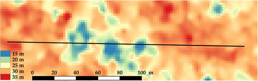
Remote Sens. 2017, 9, 205                                                                              2 of 28

different remote sensing instruments has resulted in the development of various methods and
techniques for retrieval of forest information from remote sensing data [6,7].
      Airborne laser scanning (ALS) technology has been a focus of much research in the last twenty
years, thus becoming an integral part of operational forest inventories in a number of developed
countries (e.g., Scandinavian countries, Canada, and USA) [6,8–10]. Highly accurate, three-dimensional
(3D) point clouds and canopy height models (CHMs) from ALS enable the derivation of various forest
metrics (e.g., height metrics, canopy cover or density metrics, etc.) and characterization of vertical forest
structure [11]. In combination with field reference data and established prediction models, ALS metrics
could serve for the estimation of various tree and forest inventory attributes (e.g., height, basal area,
volume, biomass, etc.) [10–16]. Generally, there are two main approaches to derive forest information
from ALS data: the area-based approach (ABA) and the individual-tree-based approach (ITBA). The
ABA uses point cloud or CHM metrics of the sampled area (e.g., plot) as input to statistical models for
forest attributes estimation [10–16]. On the other hand, the ITBA uses ALS metrics of the individual trees
that are previously delineated using segmentation methods for derivation of tree height and crown
dimensions, which are then used for calculation of other single-tree attributes (e.g., diameter at breast
height, tree volume, biomass, etc.) [13,17]. Unlike the ABA, the ITBA is not used operationally yet,
primarily due to difficulties in individual tree detection [7,18].
      Another promising remote sensing method for deriving 3D point clouds and CHMs, which
recently gained attention in forestry research, is digital aerial photogrammetry (DAP) [7,10,19].
Although aerial images have long been widely used in forest inventory (e.g., for visual
interpretation of tree and stand attributes or delineation of forest stands) [20], the recent
advancements and improvements in image quality (e.g., radiometric and geometric resolutions),
image matching algorithms, computing power and hardware sizing and capacity have promoted
their comeback in forest inventory research [3,10]. Compared to ALS, photogrammetric aerial
surveys have lower costs [21] and, in many European countries including Croatia, aerial images are
usually updated on a regular basis for topographic purposes [22]. By image matching of aerial stereo
images, digital surface models (DSMs) of similar quality and accuracy to ALS-based DSMs can be
derived [21,23]. To obtain a normalized point cloud (height above ground) or a CHM, ground
elevation data (i.e., digital terrain model (DTM)) of a high spatial resolution is required. Unlike the
ALS technology, which can penetrate through the forest canopy and derive an accurate DTM of high
spatial resolution, DAP is unable to determine ground elevation information under the dense forest
canopy. When a DTM is available, primarily from the ALS technology or stereo-photogrammetry,
cartography, and/or field surveys, the normalized point clouds or CHMs are generated by
subtracting DTMs from corresponding DSMs or point clouds. The normalized image-based point
clouds and CHMs can then serve as a basis for deriving various forest attributes in the same manner
as ALS data by using ABA or ITBA approaches.
      A number of recent studies emphasized the great potential of dense point clouds and DSMs
derived by image matching of digital aerial stereo images in combination with accurate DTMs for
the CHMs and forest attributes estimation [3,19,22,24–27]. Moreover, comparison studies which
evaluated different remote sensing data considered this image-based approach as a cost-effective
alternative to ALS in forest inventory applications [10–12,28–34]. Most of the studies where the
accuracy of forest attributes estimation is critical were evaluated mainly at the plot level. To date,
only several studies published in peer-reviewed literature [3,10,24,30,34] evaluated forest attributes
at the stand level (Table 1). Mainly, the stand level attributes were calculated by averaging plot level
attributes in other studies. There were several studies where the satellite retrievals at stand level
were used in assessment of forest attributes (e.g., [35,36]); however, to the best of the authors’
knowledge, no previous studies dealing with image matching of digital aerial images used the
metrics of an entire stand for the estimation of forest attributes at the stand level. In addition, further
research over different forest types is needed to prove the applicability of DAP in forest attributes
estimation. While several studies [10,24,30,34] were conducted in boreal forests of Northern Europe
with more uniform and consistent properties, only one study was conducted [3] in mixed,
broadleaf-dominated forests of Central Europe (Germany).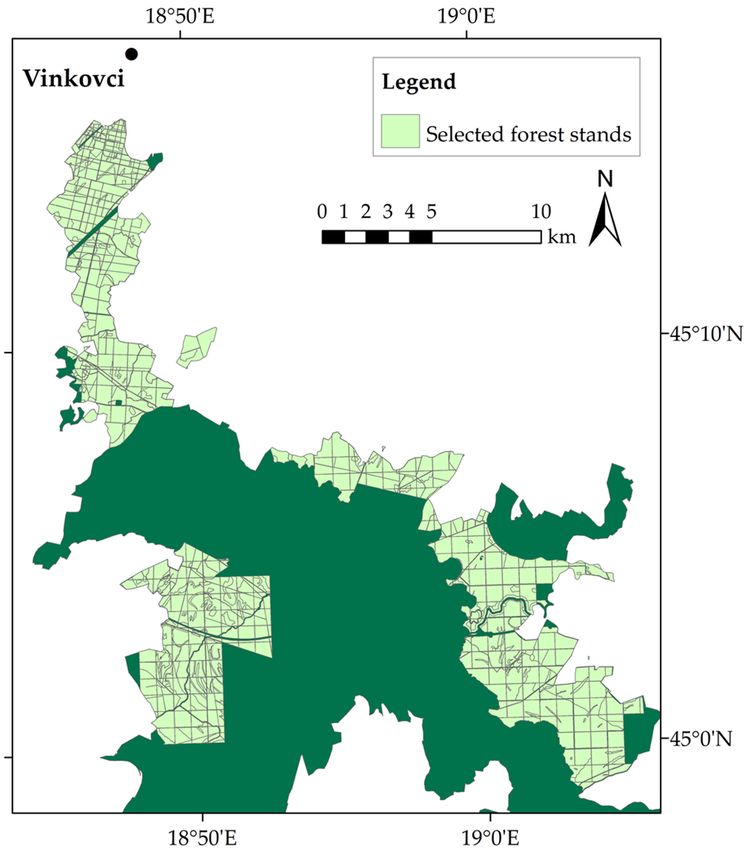
Remote Sens. 2017, 9, x FOR PEER REVIEW                                                                                                                                                                    3 of 28

     Table 1. Description and results of previous studies dealing with estimation of volume at the stand level using normalized point clouds or canopy height models
     (CHMs) derived from digital aerial images and airborne laser scanning (ALS) based digital terrain model (DTM).

           Reference                                Bohlin et al. 2012 [24]                  Rahlf et al. 2014 [10] Gobakken et al. 2015 [30]             Stepper et al. 2015 [3]     Puliti et al. 2016 [34]
         Study location                              Southern Sweden                          Southern Norway           South-eastern Norway             South-central Germany       South-eastern Norway
                                                                                             P. abies, P. sylvestris, P. abies, P. sylvestris, Betula    Fagus sylvatica, Quercus P. abies, P. sylvestris, Betula
      Dominant tree species               Picea abies, Pinus sylvestris, Betula spp.
                                                                                                  Betula spp.                       spp.                    petraea, P. sylvestris              spp.
          Camera type                                       DMC                                   UltracamX                   UltracamXp                        UltracamXp                UltracamXp
           GSD (m)                     0.48                 0.48                  0.12                 0.20                         0.17                             0.20                       0.17
          Overlap (%)                 60/30                80/30                 80/60                60/20                        80/30                           75/30               80/30            60/30
                                                                                                                                                        Remote Sensing Software       Agisoft          Agisoft
       Matching software          Match-T DSM          Match-T DSM            Match-T DSM     NGATE (SocetSet)               Match-T DSM
                                                                                                                                                               Package Graz          PhotoScan PhotoScan
                                                                                                                                                         Multiple         Random                      Multiple
         Regression type          Multiple linear     Multiple linear      Multiple linear   Linear mixed effects           Multiple linear                                        Multiple linear
                                                                                                                                                           linear          forests                     linear
  Type of independent variables      H, CC, T             H, CC, T               H, CC               H, CC                       H, CC                  H, V, CC, SP H, V, CC, SP        H                H
                                                                                                                                                                                                     Independe
       Validation method              Cross                Cross                 Cross               Cross                    Independent                  Cross            Cross   Independent
                                                                                                                                                                                                          nt
          MD (m3∙ha−1)                 3.6                  1.7                  −1.8                  -                            -                        2.9             −8.2       −0.9             1.5
           MD% (%)                     1.4                  0.7                  −0.7                  -                            -                        0.9             −2.6       −0.4             0.6
         RMSE (m3∙ha−1)                32.8                 32.6                 36.2                 33.8                          -                       46.7             43.9       31.2             35.9
          RMSE% (%)                    13.1                 13.0                 14.5                 18.1                      13.1–17.4                   14.8             13.9       13.4             15.4
     GSD: Ground Sampling Distance; RMSE: root mean square error; RMSE%: relative root mean square error; MD: mean difference; MD%: relative mean difference;
     H: height metrics; CC: canopy cover (density) metrics; T: texture metrics; SP: spectral metrics derived from orthoimages.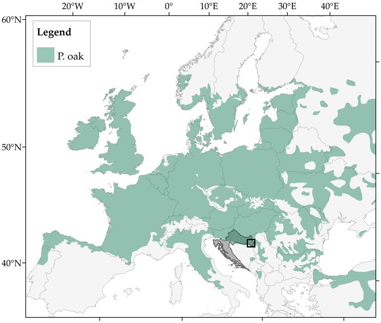
Remote Sens. 2017, 9, 205                                                                            4 of 28

      The goal of the present study is to investigate the applicability of image-based CHM for forest
attributes estimation and forest inventory at the stand level, with a special focus on the estimation of
stand-level merchantable volume of even-aged pedunculate oak (Quercus robur L.) forests. The
stand-level approach enables the use of information from existing forest management plans for
model selection and parameterization, thus overcoming the need for field measurements and
additional costs. The method that we present in this study can be universally applied, provided that
aerial surveys and forest inventory surveys were conducted simultaneously, which usually is the
case (e.g., if forest inventory interval is 10 years, it usually means that approximately 10% of the area
of managed forests is measured each year). The impact of different spatial resolutions of CHM (1 m,
2 m, and 5 m) on the stand-level volume estimates is evaluated based on the ground reference data.
For that purpose, the stand-level volume estimation models based on CHM metrics of the entire
stand are generated. In addition, the inclusions of several variables obtained from forest
management plans (stand age, soil type, site index, and phytocenological type) in the volume
estimation models are examined. Stand volume is one of the most important inventory attributes
and is crucial for understanding the dynamics and productive capacity of forest stands, as well as to
manage their use within the limits of sustainability [37,38]. Pedunculate oak is a key tree species of
European forests [39], and yet, it has not been the subject of previous similar studies. Overall, this
study attempts to provide fast, simple and low-cost photogrammetric approach for stand-level
volume estimation based on existing data (aerial images, DTM data, field data).

2. Materials and Methods

2.1. Study Area
     The research was conducted in the state-owned managed forests of Spačva basin located in
eastern Croatia (Figure 1). Covering the total area of approximately of 40,000 ha, Spačva basin is one
of the largest coherent complexes of lowland pedunculate oak forests in Europe [40]. Even-aged
pedunculate oak forests of different age classes ranging from 0 to 160 years are the main forest type,
which together occupy 96% of the forest area of Spačva basin [41]. The oak stands of the area are less
often pure and mainly mixed with other tree species (Fraxinus angustifolia Vahl., Alnus glutinosa (L.)
Geartn., Carpinus betulus L.) The stands are of high quality with site index I or II and they are actively
managed for sustained timber in 140-year rotations, ending with two or three regeneration fellings
during the last 10 years of the rotation. The regeneration fellings are implemented when old stands
produce seeds from which future young stands are raised. After successful natural regeneration and
stand establishment, silvicultural treatments are carried out throughout the rotation.
     The study area is characterized by flat terrain, with ground elevations ranging from 77 to 91 m a.s.l.
The hydromorphic soils (pseudogley, hypogley, humogley, and semigley) prevail, while
automorphic soils (luvisol) occur only on micro-elevations. According to Köppen classification, the
climate of the area is temperate and warm rainy with a mean annual temperature of 10.2 °C and a
precipitation of 709 mm·y−1 [42].

2.2. Field Reference Data
     Out of 13 management units in the Spačva basin, 6 management units with a total of 548 even-aged
pedunculate oak stands covering the area of 11,261.85 ha were selected for this research (Figure 1). In
order to enable comparison between field data and estimates from CHMs, the idea was to select
those stands, i.e., management units, in which the regular forest inventories (field measurements)
were conducted within one year of the image acquisition (2010–2012).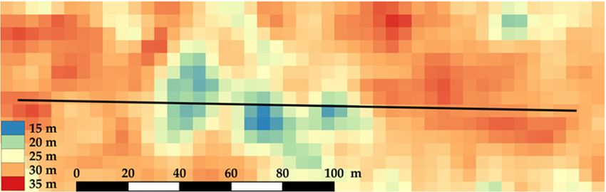
Remote Sens. 2017, 9, 205                                                                                    5 of 28

                            (a)

                                                                                  (c)

                            (b)
      Figure 1. (a) Distribution map of pedunculate oak (Quercus robur L.) in Europe [43]; (b) location of the
      Spačva basin in Croatia; and (c) spatial distribution of 548 selected even-aged pedunculate oak
      stands within the Spačva basin.

     The field data used in this study were collected according to the Regulation on Forest
Management (Official Gazette 111/06, 141/08) during the period 2010–2012 as part of the regular
forest inventories conducted by national forestry company (Croatian Forests Ltd.). All stands above
20 years of age were systematically sampled with circular plots and minimum sampling intensity of
5%. The circular sample plots had an area of 500 m2 (radius = 12.62 m), thus, at least, two plots were
established per ha. Old stands, which were prescribed for the regeneration felling in the following
ten years, were measured with 100% intensity (i.e., all trees in the stand). Diameter at breast height
(dbh) on the trees in the sampled plots, and in the old stands, was measured for all trees with dbh ≥
10 cm. At least 5 to 10 tree heights per a dbh class (5 cm gradation) were measured for each species in
each group of stands. The stands’ grouping was based on site index and stand age. The site index,
which presents potential productivity of forest stands, was determined for each stand using
Croatian growth-yield tables [44], which included stand age and mean tree height as entries. Based
on tree height and dbh measurements, the species-specific height curves (i.e., height–dbh models)
were constructed by fitting Michailloff’s function [45]. The merchantable tree volume (up to a
diameter of 7 cm overbark) of each sampled tree was calculated from field-measured dbh and tree
height estimated from species-specific height curves using the Schumacher–Hall equation [46] and
parameters from Croatian two-entry (dbh and height) volume tables [47–50]. The mean dbh and
mean height for each forest stand were calculated by averaging data of all sampled trees in the
stand, whereas stand density, basal area, and stand volume were calculated by summing the tree
data and dividing them by the total area of all plots within the stand. To reduce possible
uncertainties due to the time span between the field measurements and the aerial surveys, which
was for some parts of the study area up to one year, it was decided to exclude the stands younger
than 30 years from further analyses. Namely, very young stands have a significant share of trees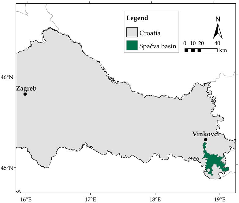
Remote Sens. 2017, 9, 205                                                                           6 of 28

with dbh thinner than the taxation limit (dbh ≥ 10 cm), and one-year ingrowth in those stands can
considerably contribute to the stand volume [51].
     A summary of the calculated stand-level forest attributes is presented in Table 2. Stand-level
merchantable volume was used in the models development and validation as a ground-truth
reference data. For those stands which were inventoried in 2010, the stand volume in 2011 was
calculated by adding an annual increment to volume from 2010. The stand volume in 2011 of stands
inventoried in 2012 was calculated by subtracting annual increment from volume measured in 2012.
Fellings did not occur within selected stands for the period from 2010 to 2012, and therefore were not
included in the stand volume calculation.

      Table 2. Descriptive statistics of the stand-level forest attributes for 548 selected even-aged
      pedunculate oak stands of Spačva basin.

                         Forest Attribute         Minimum   Maximum       Mean      SD
                           Age (years)              30.0     146.0        102.8    25.7
                          Mean dbh (cm)             14.1      58.9         32.7     6.5
                         Mean height (m)            14.3      33.6         25.3     3.0
                     Stand density (trees·ha−1)     68.0     1195.0       372.0    185.7
                        Basal area (m2·ha−1)        12.2      45.0        27.6      4.6
                         Volume (m3·ha−1)           98.1     713.2        419.2    101.4

2.3. Photogrammetric Data
     Photogrammetric data, aerial images, and digital terrain data were provided by the Croatian
State Geodetic Administration (CSGA) and were used to develop DSM and DTM, respectively.
     The color infrared (CIR) 8-bit digital aerial images were acquired using the Intergraph Z/I
Imaging Digital Mapping Camera (DMC) system [52] as part of the regular national topographic
survey in August 2011. The study area was represented by 157 images with the ground sampling
distance (GSD) of approximately 30 cm. The images were collected in 11 flight lines with forward
overlaps of 60% and side overlaps of 30%. The images were block-triangulated, using the bundle
adjustment method, and post-processed, including radiometric and geometric corrections, as well as
pan-sharpening. This was done by the contractor (Geodetski zavod Ltd. Osijek, Croatia) according
to the rules of the CSGA (Product Specification 301D130). The horizontal (x, y) and vertical (z)
accuracies of the processed images were validated with ground control points (root mean square
error (RMSE) < 0.25 m and < 0.30 m, respectively).
     The digital terrain data (breaklines, formlines, spot heights and mass points), used to generate
DTM, were collected according to the rules of the CSGA (Product Specifications 301D150). The main
method for national digital terrain data collection is aerial stereo photogrammetry (aerial images of
GSD ≤ 30 cm), supported with vectorization of existing maps and field data collection (especially for
unreliable areas, which are not visible from aerial images). Data density is dependent of terrain type,
slope and surface roughness. The average distance between points in breaklines and formlines is
recommended to be 25 m, while the average distance between mass points is recommended to be
70–90 m. For flat areas, or areas covered by vegetation, the distance can be larger but not more than
120 m. For the flat terrain, which correspond to the terrain type of the research area, (Spačva basin),
the required number of points in breaklines and formlines is 400–800 points·km2, while the required
number of mass points and spot heights is 100–150 points·km2. The required absolute accuracy of
digital terrain data (including both horizontal and vertical accuracy) validated with ground control
points is < ±1 m of the standard deviation for the well-defined details and < ±2 m for not well-defined
details.
Remote Sens. 2017, 9, 205 7 of 28
2.4. Photogrammetric Processing (CHM Generation)
The photogrammetric data processing, which included the generation of DSMs, DTMs, and
CHMs, was performed using the PHOTOMOD 5.24 digital photogrammetric system (Racurs Co.,
Moscow, Russia).
DSMs were generated using the Dense DTM algorithm of PHOTOMOD DTM module. Dense
DTM is an area-based image matching algorithm that calculates the coordinates of conjugate points
between overlapping images for each pixel of the selected area using the cross-correlation approach.
The spatial resolution (pixel size) of the resulting DSM thus corresponds to the image pixel size (0.30
m × 0.30 m). A detailed description of the procedure of the DSM generation using Dense DTM, as
well as parameters settings, can be found in Balenović et al. [53]. Matching errors, i.e., spikes (points
above or below the surface) were removed from DSM using the DSM filters. The resulting gaps (null
cells) were then filled by a Smooth interpolation method. Finally, the initial raster DSM of 0.30 m
resolution (DSM0.3) was then resampled to DSMs of 1 m, 2 m, and 5 m resolutions (hereinafter
referred to as DSM1, DSM2, and DSM5). The resampling was conducted by: (a) converting the initial
DSM from raster to point format; (b) reducing the number of points by using the “thin-out”
coefficient of 3, 6 and 16; (c) creating the triangular irregular networks (TINs) from corresponding
reduced points; and (d) generating raster DSMs of 1 m, 2 m, and 5 m resolutions from corresponding
TINs. In the recently published study by Balenović and Marjanović [54], the vertical accuracy of
DMSs of different spatial resolutions (DSM1, DSM2, and DSM5) generated from the same aerial
images, was evaluated by comparing manually stereo measured elevations of 294 tree tops with the
elevations of planimetrically corresponding DSM’s points. The RMSE values for the DSM1, DSM2,
and DSM5 generated for the part of the Spačva basin (1869.33 ha) that was also included in the
present study were 0.76 m, 0.84 m, and 1.31 m, respectively.
For the DTMs generation, national digital terrain data were used. First, a TIN was created from
the digital terrain data, which was then converted through the linear interpolation into a raster
DTMs of 1 m, 2 m, and 5 m resolutions.
A raster CHMs of 1 m, 2 m, and 5 m resolutions (hereinafter referred to as CHM1, CHM2, and
CHM5) of the research area was generated by subtracting ground from surface elevation data, i.e., by
subtracting DTMs from corresponding DSMs. All pixels with heights above 45 m in CHMs were
considered as outliers and were filtered (removed). The maximum threshold of 45 m was defined
based on the maximum tree heights in the study area. The resulting gaps were then filled using a
Smooth interpolation method. Prior to the metrics extraction (explained below), and in accordance
with other similar studies [3,34], a minimum threshold of 5 m was applied to remove ground and
understorey vegetation (e.g., shrubs, small trees with dbh < 10 cm). The minimum threshold of 5 m
was defined based on the minimum height of trees with dbh ≥ 10 cm. In other words, all trees with
dbh ≥ 10 cm at the study area have heights above 5 m.
2.5. CHM Metrics
In other studies [3,10,24,30], the height and density metrics extracted from CHMs have proven
to be good predictors of various forest attributes. To extract the stand-level metrics from CHMs, the
boundaries of the selected forest stands were overlaid on CHMs. For each forest stand, both height
metrics and density metrics were extracted and calculated from each CHM. In total, 24 CHM metrics
were extracted and considered in the statistical modeling (i.e., for development of stand-level
volume models) as potential independent variables. The CHM metrics with corresponding
description and explanation of the calculation are summarized in Table 3.Remote Sens. 2017, 9, 205 8 of 28
Table 3. Metrics extracted from CHMs, calculated for each stand and used as potential independent
variables in statistical analysis (development of stand-level volume model).
CHM Metrics Description and Explanation
hmean (m) Arithmetic mean of pixels height
hSD (m) Standard deviation of pixels height
hmode (m) Mode height
Height hmax (m) Maximum height
metrics hmin (m) Minimum height
p5, p10, p20, p25, p30, p40, p50,
Height percentiles (5th, 10th, 20th, 25th, 30th, 40th,
p60, p70, p75, p80, p90, p95, p99
50th, 60th, 70th, 75th, 80th, 90th, 95th, 99th)
(m)
Ratio between area of canopy above certain height
Density CC10, CC20, CC30, CC40
threshold (10 m, 20 m, 30 m, 40 m) and stand area
(cover)
Ratio between 3D canopy surface model area and
metrics k3D
ground area
2.6. Variables from Forest Management Plans
In addition to extracted CHM metrics, several existing and easily obtainable stand variables
from Forest management plans (FMP variables) were considered in statistical modeling as potential
independent variables (Table 4).
Table 4. Existing stand variables from Forest management plans (FMP variables) used as potential
independent variables in statistical analysis (development of stand-level volume models).
Variable Description and Explanation
SA Stand age (from 30 to 146)
ST Soil type (pseudogley, hypogley, humogley, semigley, luvisol)
SI Site index (I, II)
Phytocenological type (Genisto elatae-Quercetum roburis caricetosum remotae, Genisto
PT
elatae-Quercetum roburis aceretosum tatarici, Carpino betuli-Quercetum roburis "typicum")
2.7. Development of the Stand-Level Volume Models and Validation
A multivariate linear regression approach, as explained in Bohlin et al. [24], Straub et al. [22]
and Montealegre et al. [16], was applied to develop the stand-level volume models. In total, 548
forest stands were used in the statistical analyses, out of which 274 were selected for the models’
development and the other 274 stands for the models’ validation. To reduce bias in stands’ selection,
they were categorized according to age from youngest to oldest, and then ranked. Every
odd-numbered stand was selected in the modeling while every even-numbered stand was selected
in the validation. This way, both datasets contained stands of similar ages. All the statistical analyses
were performed using the program STATISTICA 11 [55].
Prior to the modeling, the potential independent variables were selected based on Pearson
correlation coefficient (r). Among a number of potential predictors (CHM metrics and FMP
variables), only variables that were highly correlated with field estimated stand volume (r ≥ ±0.5)
were included in the backward stepwise regression. This type of regression is commonly used for
linear modeling of forest attributes based on either image-based [22,24] or ALS-based [16,56] metrics.
To justify the use of linear regression models, four principal statistical assumptions [57] were tested:
(i) linearity and additivity of the relationship between dependent and independent variables
(scatterplots of predicted vs. observed values and predicted values vs. residuals); (ii)
homoscedasticity (scatterplots of predicted values vs. residuals and residuals vs. independent
variables); (iii) normality of the error distribution (Shapiro–Wilk test [58]); and (iv) independence
(auto-correlation) of the errors (Durbin–Watson test [59]). To meet the above-mentioned conditionsRemote Sens. 2017, 9, 205 9 of 28
and achieve a linear relationship, the dependent variable (stand volume) was logarithmically
transformed, which is in agreement with other similar studies [24,34]. By applying backward
stepwise regressions and Akaike information criterion value [60], two the-best-fit models were
developed and selected for each CHM (CHM1, CHM2, CHM5) using the modeling dataset. The first
model was developed solely from CHM metrics, whereas the second model was developed from
both CHM metrics and FMP variables. The multivariate log-linear models had the following form:
ln( )= + + + ⋯+ (1)
where is the predicted stand volume (m3·ha−1); is intercept; , , …, are regression
coefficients; and , , , …, are independent variables (CHM metrics, and FMP variables).
In order to account for the bias in log-normal linear regression, bias correction ratio (CR,
Equation (2)) proposed by Snowdon [61] was calculated for each model. Several methods for
correcting bias introduced by logarithmic transformation described in literature [61–64] were
considered. Snowdon’s CR was selected as the most suitable for application in this research. CR was
calculated as the ratio of the mean of the observed stand volumes ( ) and the mean of the predicted
stand volumes ( , Equation (2)). Bias corrected volume ( ), was calculated using Equation (3).
= (2)
= × (3)
The models were validated using the independent validation dataset. The stand-level volume
estimates were compared with the corresponding field data (stand volume from field inventories).
The goodness-of-fit of the stand-level volume models was evaluated by the adjusted coefficient of
determination (R2adj) calculated using raw (log-transformed) data and graphical analyses (observed
vs. predicted values, residuals vs. independent variables). To evaluate the accuracy of the models’
estimates, the root mean square error (RMSE) (Equation (4)) and relative root mean square error
(RMSE%) (Equation (5)), as well as the mean difference (MD) (Equation (6)) and relative mean
difference (MD%) (Equation (7)) were calculated:
∑ ( ′ − )
= (4)
% = × 100 (5)
∑ ( ′ − )
= (6)
% = × 100 (7)
where ′ is the predicted volume of stand i, is the observed (field estimated) volume of stand i, n
is the number of stands, and is the mean of the observed values.
The accuracy measures were calculated for the entire modeling and validation datasets as well
as for each stand development stage. According to the Regulation on Forest Management (Official
Gazette 111/06, 141/08), stands of the research area were classified as young (30–70-year-old),
middle-aged (71–93-year-old), mature (94–120-year-old), and old stands (≥121-year-old).
Additionally, the performance of the regression models with double-log transformation, i.e.,
with logarithmically transformed dependent and independent variables, was also evaluated.
3. Results
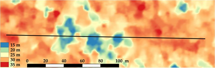
Examples of the generated CHMs for a sample area of 1.74 ha are given in Figure 2a–c. As
expected, CHM1 provides the highest discrimination of details. While all three CHMs enableRemote Sens. 2017, 9, 205 10 of 28
visualization of larger gaps in the canopy, the smaller gaps cannot be determined by CHM5 (Figure 2a–
c). This is also evident in Figure 2d which shows a comparison of CHMs’ profiles through exemplary
forest stand (marked with black lines in Figure 2a–c). CHM2 provides a very similar profile with
some minor differences from CHM1 at the peak values. On the other hand, CHM5 notably differ from
CHM1 and CHM2. Namely, the areas of forest surface with greater heights are underestimated, while
the areas of lower heights are considerably overestimated by CHM5.
(a)
(b)
(c)
(d)
Figure 2. Examples of CHMs generated at the different spatial resolution: (a) CHM1 (1 m); (b) CHM2
(2 m); and (c) CHM5 (5 m); and (d) the profile across a segment of the research area for each CHM.
Table 5 shows the Pearson correlation coefficients (r) between stand volume from
measurements from field inventories and potential predictors (i.e., stand-level metrics extracted
from each CHM and variables obtained from FMPs), whereas the correlation coefficients between
the potential predictors (independent variables) are presented in Table A1. Among 24 considered
CHM metrics, for all CHMs, the same 18 metrics (hmean, hmode, hmax, p10, p20, …, p99, CC20, CC30) fulfillRemote Sens. 2017, 9, 205 11 of 28
required criteria (p < 0.05, r ≥ ±0.5) for entering the further modeling. Out of four FMP variables, a
strong correlation with stand volume is identified only for stand age (SA). All selected variables
result in very similar, almost identical r values for all CHMs. Accordingly, for each CHM, 19
identical potential independent variables (18 CHM metrics and one FMP variable) are selected and
included in the backward stepwise regression.
Table 5. Pearson correlation coefficients (r) between the potential predictors (CHM metrics and FMP
variables) and stand volume from field measurements calculated on the modeling dataset.
Stand Volume (m3∙ha−1)
Variable
CHM1 CHM2 CHM5
hmean (m) 0.83 * 0.83 * 0.83 *
hSD (m) 0.42 * 0.42 * 0.39 *
hmode (m) 0.83 * 0.83 * 0.84 *
hmax (m) 0.66 * 0.67 * 0.70 *
hmin (m) 0.13 * 0.13 * 0.13 *
p5 (m) 0.43 * 0.43 * 0.47 *
p10 (m) 0.59 * 0.59 * 0.62 *
p20 (m) 0.73 * 0.73 * 0.74 *
p25 (m) 0.76 * 0.76 * 0.77 *
p30 (m) 0.78 * 0.79 * 0.79 *
p40 (m) 0.82 * 0.82 * 0.82 *
p50 (m) 0.84 * 0.84 * 0.83 *
CHM metrics
p60 (m) 0.84 * 0.84 * 0.84 *
p70 (m) 0.84 * 0.84 * 0.84 *
p75 (m) 0.84 * 0.84 * 0.84 *
p80 (m) 0.84 * 0.84 * 0.84 *
p90 (m) 0.83 * 0.83 * 0.83 *
p95 (m) 0.83 * 0.83 * 0.83 *
p99 (m) 0.80 * 0.81 * 0.81 *
CC10 0.17 * 0.17 * 0.18 *
CC20 0.79 * 0.79 * 0.79 *
CC30 0.54 * 0.54 * 0.51 *
CC40 0.07 ns 0.07 ns 0.04 ns
k3D 0.40 * 0.40 * 0.36 *
SA (years) 0.77 * 0.77 * 0.77 *
ST −0.19 * −0.19 * −0.19 *
FMP variables
SI 0.09 ns 0.09 ns 0.09 ns
PT 0.17 * 0.17 * 0.17 *
* Correlations are significant at p < 0.05; ns: not significant correlations (p ≥ 0.05).
For each CHM, two best fit stand-level volume models were developed and selected based on
the backward stepwise regression and Akaike information criterion (Table A2). Development of the
first model was based only on previously selected CHM metrics (hmean, hmode, hmax, p10, p20, …, p99,
CC20, CC30), whereas in the development of the second model SA was also included. All models and
their parameters exhibit highly significant results (p < 0.001). A similar set of independent variables
was included in all models. Namely, in all models one or two height percentiles were included,
along with hmax and CC30.
Table 6 shows results of stepwise regression and validation for six selected stand-level volume
models. The R2adj for the modeling dataset for the first (1-A, 2-A, 5-A; hereinafter referred to as A
models) and second (1-B, 2-B, 5-B; hereinafter referred to as B models) group of models is 0.83 and
0.84, respectively, indicating a good model fit (Table 6). For the validation dataset, both groups of
models exhibit just slightly lower R2adj values than for modeling dataset. R2adj for modeling andRemote Sens. 2017, 9, 205 12 of 28
validation dataset differ by 500 m3·ha−1. To further
characterize models’ performance and relationships between dependent and independent variables,
scatterplots of residuals vs. independent variables are given in Appendix B (Figure A1).
Observed by models’ type, it can be noted that models developed solely from CHM metrics (A
models) produce slightly less precise volume estimates than the models developed from both CHM
metrics and SA (B models) (Table 6). This can be observed for all CHMs. Compared to models 1-A,
2-A, and 5-A, the R2adj values for models 1-B, 2-B, and 5-B are increased by 0.1, 0.3, and 0.2,
respectively, whereas the RMSE% values are decreased by 0.55%, 0.75%, and 0.62%, respectively.
However, compared to models 1-A, 2-A, and 5-A, the MD% values for models 1-B, 2-B, and 5-B are
increased by −0.08, −0.14, and −0.04, respectively.
The obtained results are similar for all three CHM resolutions (1 m—CHM1, 2 m—CHM2, and 5
m—CHM5) (Table 6). For instance, the differences between the RMSE% for the best performing
model 2-B derived using metrics extracted from CHM2, and models derived using metrics extracted
from CHM1 (model 1-B) and CHM5 (model 5-B) are 0.06% and 0.11%, respectively.
Figure 4 shows validation results by stand development stages. Overall, the highest RMSEs%
are calculated for young stands (16.69%–20.65%), followed by mature (12.86%–13.45%) and
middle-aged stands (10.82%–12.73%), whereas the lowest RMSE%, i.e., the highest accuracy, are
calculated for old stands (10.30%–11.42%). Except for the young stands, for which somewhat greater
differences between RMSE% of A and B models can be noticed (3.35%–3.96%), the differences
between A and B models for all other development stages are considerably smaller (middle-aged:
0.87%–1.45%, mature: 0.26%–0.50%, old: 0.55%–0.84%). Similar to the complete dataset analyses, the
differences between the CHM datasets of different resolutions (1 m, 2 m, and 5 m) for each
development stage are negligible.Remote Sens. 2017, 9, 205 13 of 28
Unlike the RMSE% values, the MD% values vary noticeably for different development stages, as
well as for different models’ types within each development stage. For the young stands, the values
are overestimated for both models, ranging from 3.83% to 5.08% and from 0.84% to 1.93% for the A
and B models, respectively. For the middle-aged stands, the MD% values are also overestimated for
the A models ranging between 4.02% to 4.86%, while the MD% values for the B models are very close
to 0, ranging from −0.56% to 0.27%. For these two development stages (young, middle-aged) it is
evident that the inclusion of SA into the B models considerably decreases the models’ bias
(underestimations). On the other hand, for the mature stands, both model types result in
underestimated MD% values with a similar range. The MD% values for the A and B models range
from −1.66% to −2.06% and from −1.57% to −1.99%, respectively. Furthermore, for the old stands, A
models produce the underestimated values (−1.10% to −2.87%), whereas the inclusion of SA into the
B models results in decreased MD% values, ranging from −0.64% to 1.07%.
700 Model 1-A 700 Model 1-B
600 600
500 500
400 400
300 300
200 200
100 100
100 200 300 400 500 600 700 100 200 300 400 500 600 700
700 Model 2-A 700 Model 2-B
600 600
500 500
Observed
V 400 400
(m3·ha−1) 300 300
200 200
100 100
100 200 300 400 500 600 700 100 200 300 400 500 600 700
700 Model 5-A 700 Model 5-B
600 600
500 500
400 400
300 300
200 200
100 100
100 200 300 400 500 600 700 100 200 300 400 500 600 700
Predicted V (m3·ha−1)
Figure 3. Observed vs. predicted stand volume (V) for six selected stand-level volume models
(validation dataset) described in Table 5. The solid line represents fitted linear model.Remote Sens. 2017, 9, 205 14 of 28
70 25
(a) (b) 1-A 1-B
60 2-A 2-B
20 5-A 5-B
50
RMSE (m3∙ha-1)
15
RMSE (%)
40
30 10
20
5
10
0 0
Young Middle-aged Mature Old Young Middle-aged Mature Old
20 6
(c) (d)
15
4
10
2
MD (m3∙ha-1)
5
MD (%)
0 0
-5
-2
-10
-15 -4
Young Middle-aged Mature Old Young Middle-aged Mature Old
Stand Development Stage
Figure 4. Validation results by stand development stages (young, middle-aged, mature, old): (a) root
mean square error (RMSE); (b) relative root mean square error (RMSE%); (c) mean difference (MD);
and (d) relative mean difference (MD%).
In general, the regression models with the double-log transformation used to model stand-level
volume do not yield any better results than the log-linear regression models. Detailed results of the
double-log analysis can be found in Appendix C (Tables A3 and A4, Figures A2 and A3).
4. Discussion
Despite the proven applicability of ALS technology for operational forest inventory, the
high-cost of ALS surveys is a limiting factor that impedes its widespread use. In many countries,
including Croatia, the national ALS surveys have not been conducted yet. Thus, aerial images,
which are regularly updated in many European countries [22], present an alternative to ALS
technology. The digital terrain data (breaklines, formlines, spot heights and mass points) used to
generate DTM in this study present the national standard and they are the only available DTM data
for Croatia. It is well known that the photogrammetrically-based (stereo-mapping) DTM of forested
areas has a lower accuracy than ALS-based DTM because of the ground being obscured by
vegetation [12,21]. However, since the research area in this study is characterized by flat terrain, it
can be assumed that DTM derived from digital terrain data could be of satisfactory accuracy.
Nevertheless, many countries may benefit from studies like this one where the main concern is to
explore the applicability of the existing photogrammetric data to generate CHM and to estimate
stand volume of different forest types.
Previous studies [3,10,24,30,34], regardless of the data used (ALS or aerial images), mostly
utilized plot-level metrics to estimate volume at stand level, while in this study we have estimated
the stand volume based on the stand-level metrics. To the best of the authors’ knowledge, this
research is the first that has focused on stand-level metrics extracted from the image-based CHM,
i.e., from CHM that is completely derived from photogrammetric data. Since it is completely basedRemote Sens. 2017, 9, 205 15 of 28
on existing data (aerial images, DTM data, field data), this approach is considered as a low-cost
alternative. As such, the study serves as a basis for other studies where ALS technology is limited
(i.e., in countries and regions which do not have access to ALS data, and will probably not have
access in the near future either). Furthermore, to apply this stand-level approach, the acquisition of
precise location (which is not an easy task in dense forests) of the reference field plots is not
necessary. This presents an additional benefit for inventories of large areas to be completed in a
short period of time. It should be emphasized that the aim of this approach is not to replace field
inventories or plot-level remote sensing inventories which also requires a certain amount of field
reference data collected at the same time as remote sensing data. As already noted, regular field
forest inventories are usually conducted at 10-year intervals, whereas aerial images in Croatia and
many other European countries are regularly updated every 3–5 years. Therefore, provided that
aerial survey and regular forest inventory of some specific area (forest type) were conducted
simultaneously (which was the case for the part of the Spačva basin in 2011), stand-level models
could be derived using image-based CHM metrics and existing field inventory data. This approach,
i.e., these models could be then used to estimate stand volume on other sites of the same forest type
or for the same area after next aerial survey. Concretely, for the Spačva basin, the stand-level
approach could be applied using new images from 2016, which will be available from CSGA soon.
This means that fast and reasonably accurate stand volume estimates for Spačva basin could be
obtained five years before regular forest inventory (2021–2022). Such more frequently updated
information on forests could serve as a great support to practical management activities, as well as
for monitoring of forest state and condition.
Regardless of the spatial resolution of the CHM datasets, the metrics extracted from each CHM
exhibit a similar, almost identical correlation with the stand volume derived from field
measurements (Table 5). This leads to the conclusion that the uncertainties involved in the modeling
of forest surface, namely under- and overestimations obtained for CHM5, are consistent throughout
the area. As a result, by applying the backward stepwise regression, the similar set of independent
variables are successfully selected and included in the stand-level volume models for all CHM
resolutions (Table A2). As previously mentioned, the CHM metrics (e.g., height metrics, and canopy
cover metrics) selected and included in the final stand-level modeling are similar to metrics used for
predicting plot-level volume in other studies [3,10,24,30,34]. However, while in the present study the
SA has been used in B models, variables in other studies, such as texture metrics derived from CHM
rasters [24] or spectral metrics derived from orthoimage [3], were used in addition to height and
canopy cover metrics extracted from CHMs.
This study (Table 6, Figure 3) suggests that models with CHM metrics and SA as independent
variables (B models) have slightly better performance overall than models based solely on CHM
metrics (A models). The inclusion of SA, in addition to CHM metrics, decreased RMSE% by 0.55%
(1-B), 0.75% (2-B), and 0.62% (5-B). This step of the research is of particular importance because the SA
is, for even-aged stands, usually known, or easily obtainable variable, from the existing forest
management plans. Therefore, it may be considered as an additional predictor of stand volume in
future studies.
Among all tested models, model 2-B, with metrics extracted from CHM2 and SA as independent
variables, exhibits the best performance (RMSE% = 12.53%). On the other hand, the worst
performance is observed for model 5-A (RMSE% = 13.28%) with metrics extracted from CHM2 as only
independent variables, which is in agreement with other studies [3,10,24,30,34]) where the estimated
stand volume using image-based point clouds or CHMs had RMSE% from 13.0% to 18.1%. Due to a
number of differences between studies (e.g., site characteristics, forest structure, camera and image
characteristics, matching software, etc.), precise comparison of the results is not possible. The
agreement between the results of this and previous studies [3,10,24,30,34] suggests that the
stand-level metrics extracted from the image-based CHMs can be used for the estimation of stand
volume with similar or even slightly better accuracy than plot-level metrics. Moreover, the obtained
results are also in agreement with the recent studies based on ALS data. For example, Rahlf et al.Remote Sens. 2017, 9, 205 16 of 28
[10], Gobakken et al. [30], and Puliti et al. [34] estimated volume at stand level using ALS data with
RMSE% of 12.4%, 11.6%, and 13.3%, respectively.
Concerning the different resolutions (1 m, 2 m, 5 m) of CHMs used in this research, very similar
results were obtained for all three CHMs (CHM1, CHM2, CHM5) (Table 6, Figure 3). This implies that
stand-level metrics extracted from all observed CHM resolutions (1 m, 2 m, 5 m) can provide
reasonably accurate stand volume estimates. Similarly, Bohlin et al. [24] did not find improvements
in estimation accuracy of forest stand attributes using point clouds derived from images of lower
GSD (Table 1). Although the increase in resolution may result in better accuracy [30], CHMs of lower
spatial resolution facilitate faster data manipulation and processing, especially for larger areas.
Images of lower spatial resolutions or point clouds of lower densities, together with the lower
amount of extracted metrics, occupy a smaller storage size than CHMs of high spatial resolution or
very dense point clouds. Therefore, the trade-off between spatial resolution and required accuracy
for a given area should be identified.
With respect to the stand development stages, the highest accuracy is obtained for old stands
and the lowest accuracy for young stands (Figure 4). Although one could consider such a trend as
the uncertainty of the proposed approach, it is in accordance with the findings of Gobakken et al.
[30]. Namely, young stands of the research area are very dense with homogeneous structure and
mostly without the presence of gaps in crowns. Therefore, the independent variable CC30, which
describes density (cover) of stands, has a less significant role in the performance of A models for
young stands, resulting in the stand volume estimates of lower accuracy. This confirms our findings
that the inclusion of SA as additional predictors in B models considerably improves estimation
accuracy in young and middle-aged stands (Figure 4).
5. Conclusions
This research confirmed the great potential of digital aerial photogrammetry for stand-level
forest inventory when fast, simple and low-cost approach based on existing data is needed. Image
matching of existing digital aerial images from a national topographic survey, as well as
interpolation of existing DTM data, were successfully applied to generate CHMs of different spatial
resolutions (1 m, 2 m, and 5 m) for the area of even-aged pedunculate oak forests. For the first time,
the stand-level metrics extracted from image-based CHMs were used to estimate the stand volume.
The estimation accuracies were similar or even slightly better compared to those obtained from
previous studies in which stand volume estimates were based on plot-level metrics. The validation
results showed that the inclusion of stand age as an independent variable in addition to CHM
metrics slightly improved the accuracy of stand volume estimates. Observed by stand development
stages, these improvements were considerable for young and middle-aged stands, and they were
negligible for mature and old stands. As stand age is an easily obtainable variable, it is recommended
to use it for volume estimation, at least for young and middle-aged stands. The comparison between
the different CHM’s resolutions (1 m, 2 m, 5 m) used for metrics extraction and volume estimation,
showed that all observed CHM resolutions were capable of providing reasonably accurate volume
estimates at the stand level. Additionally, this research revealed that in the absence of ALS-based DTM
data, the existing digital terrain data, commonly collected by stereo mapping and field survey, could
be readily used for DTM and CHM generation for flat terrains and lowland forests. This research
serves as a basis for future studies where the applicability of the stand-level CHM approach should be
tested for estimating other important forest stand attributes such as mean tree height, mean dbh, stand
density, basal area, and biomass, across different forest types. The prediction potential of other
variables obtainable from aerial images (e.g., color information/spectral metrics) and CHMs (e.g.,
texture metrics) should be examined.Remote Sens. 2017, 9, 205 17 of 28 Acknowledgments: This research has been supported by the Croatian Science Foundation under the project “Estimating and Forecasting Forest Ecosystem Productivity by Integrating Field Measurements, Remote Sensing and Modeling” (HRZZ UIP-11-2013-2492). The authors wish to thank Dr. Maša Zorana Ostrogović Sever for help in data processing. We also thank the Anonymous Reviewers for the valuable comments that helped us to improve the quality of the manuscript. Author Contributions: I.B., A.S.M. and H.M. conceived and designed the research; I.B. performed photogrammetric processing; I.B. and H.M. performed statistical analysis; I.B., A.S.M. and H.M. analyzed the results; and I.B., A.S.M. and H.M. wrote the paper. Conflicts of Interest: The authors declare no conflict of interest.
Remote Sens. 2017, 9, x 17 of 28
Appendix A
Table A1. Pearson correlation coefficients (r) between the independent variables (CHM metrics and FMP variables) calculated on the modeling dataset for the each
CHM resolution (1 m—CHM1, 2 m—CHM2, 5 m—CHM5). Correlations marked with * are significant at p < 0.05.
CHM1 hmean hSD hmode hmax hmin p5 p10 p20 p25 p30 p40 p50 p60 p70 p75 p80 p90 p95 p99 CC10 CC20 CC30 CC40 k3D SA ST SI PT
hmean 1.00 0.36 * 0.95 * 0.82 * 0.15 * 0.63 * 0.80 * 0.93 * 0.96 * 0.97 * 0.99 * 0.99 * 0.99 * 0.98 * 0.97 * 0.97 * 0.95 * 0.94 * 0.92 * 0.29 * 0.92 * 0.70 * 0.14 * 0.37 * 0.80 * −0.26 * 0.14 * 0.19 *
hSD 1.00 0.57 * 0.60 * −0.32 * −0.42 * −0.24 * 0.03 0.12 0.20 * 0.33 * 0.42 * 0.49 * 0.54 * 0.56 * 0.57 * 0.61 * 0.62 * 0.64 * −0.45 * 0.24 * 0.51 * 0.37 * 0.93 * 0.60 * −0.36 * 0.13 * 0.26 *
hmode 1.00 0.85 * 0.05 0.44 * 0.62 * 0.80 * 0.85 * 0.88 * 0.94 * 0.97 * 0.98 * 0.98 * 0.98 * 0.98 * 0.97 * 0.97 * 0.95 * 0.16 * 0.85 * 0.73 * 0.20 * 0.56 * 0.84 * −0.32 * 0.16 * 0.22 *
hmax 1.00 −0.11 0.32 * 0.48 * 0.65 * 0.70 * 0.74 * 0.80 * 0.83 * 0.85 * 0.86 * 0.87 * 0.87 * 0.88 * 0.89 * 0.90 * 0.08 0.69 * 0.73 * 0.32 * 0.64 * 0.78 * −0.35 * 0.14 * 0.23 *
hmin 1.00 0.40 * 0.31 * 0.22 * 0.19 * 0.17 * 0.13 * 0.11 0.09 0.08 0.07 0.07 0.06 0.05 0.03 0.31 * 0.18 * 0.03 −0.11 −0.24 * 0.01 −0.02 −0.10 −0.02
p5 1.00 0.93 * 0.79 * 0.74 * 0.70 * 0.63 * 0.57 * 0.52 * 0.49 * 0.47 * 0.46 * 0.43 * 0.41 * 0.38 * 0.71 * 0.66 * 0.28 * −0.14 * −0.33 * 0.29 * −0.01 0.02 −0.01
p10 1.00 0.94 * 0.91 * 0.88 * 0.81 * 0.75 * 0.71 * 0.67 * 0.65 * 0.64 * 0.61 * 0.59 * 0.56 * 0.63 * 0.79 * 0.42 * −0.07 −0.19 * 0.45 * −0.06 0.06 0.05
p20 1.00 0.99 * 0.98 * 0.95 * 0.91 * 0.87 * 0.84 * 0.83 * 0.81 * 0.78 * 0.76 * 0.74 * 0.49 * 0.89 * 0.56 * 0.03 0.05 0.63 * −0.13 * 0.11 0.10
p25 1.00 0.99 * 0.97 * 0.94 * 0.91 * 0.88 * 0.87 * 0.86 * 0.83 * 0.81 * 0.79 * 0.44 * 0.90 * 0.60 * 0.07 0.13 * 0.68 * −0.16 * 0.12 * 0.12 *
p30 1.00 0.99 * 0.96 * 0.94 * 0.92 * 0.91 * 0.89 * 0.87 * 0.86 * 0.83 * 0.40 * 0.91 * 0.64 * 0.09 0.21 * 0.72 * −0.18 * 0.13 * 0.14 *
p40 1.00 0.99 * 0.98 * 0.97 * 0.96 * 0.95 * 0.93 * 0.92 * 0.90 * 0.31 * 0.92 * 0.69 * 0.13 * 0.33 * 0.78 * −0.23 * 0.14 * 0.17 *
p50 1.00 0.99 * 0.99 * 0.98 * 0.98 * 0.97 * 0.95 * 0.93 * 0.26 * 0.91 * 0.72 * 0.17 * 0.42 * 0.82 * −0.27 * 0.15 * 0.19 *
p60 1.00 0.99 * 0.99 * 0.99 * 0.98 * 0.97 * 0.96 * 0.22 * 0.90 * 0.73 * 0.19 * 0.49 * 0.84 * −0.30 * 0.15 * 0.21 *
p70 1.00 0.99 * 0.99 * 0.99 * 0.99 * 0.97 * 0.18 * 0.88 * 0.74 * 0.20 * 0.54 * 0.85 * −0.32 * 0.15 * 0.22 *
p75 1.00 0.99 * 0.99 * 0.99 * 0.98 * 0.16 * 0.88 * 0.74 * 0.21 * 0.56 * 0.85 * −0.33 * 0.15 * 0.23 *
p80 1.00 0.99 * 0.99 * 0.98 * 0.15 * 0.87 * 0.75 * 0.22 * 0.58 * 0.86 * −0.34 * 0.15 * 0.24 *
p90 1.00 0.99 * 0.99 * 0.12 * 0.86 * 0.75 * 0.23 * 0.61 * 0.86 * −0.35 * 0.15 * 0.24 *
p95 1.00 0.99 * 0.10 0.84 * 0.76 * 0.23 * 0.63 * 0.86 * −0.37 * 0.15 * 0.25 *
p99 1.00 0.08 0.82 * 0.76 * 0.26 * 0.65 * 0.86 * −0.39 * 0.14 * 0.25 *
CC10 1.00 0.34 * 0.05 −0.09 −0.39 * 0.04 0.06 0.02 −0.08
CC20 1.00 0.40 * 0.04 0.25 * 0.76 * −0.08 0.19 * 0.13 *
CC30 1.00 0.28 * 0.52 * 0.55 * −0.49 * −0.03 0.21 *
CC40 1.00 0.40 * 0.18 * −0.18 * −0.04 0.19 *
k3D 1.00 0.61 * −0.41 * 0.10 * 0.29 *
SA 1.00 −0.23 * 0.37 * 0.21 *
ST 1.00 0.04 −0.30 *
SI 1.00 −0.16 *
PT 1.00
CHM2 hmean hSD hmode hmax hmin p5 p10 p20 p25 p30 p40 p50 p60 p70 p75 p80 p90 p95 p99 CC10 CC20 CC30 CC40 k3D SA ST SI PT
hmean 1.00 0.35 * 0.95 * 0.82 * 0.15 * 0.63 * 0.80 * 0.93 * 0.96 * 0.97 * 0.99 * 0.99 * 0.99 * 0.98 * 0.97 * 0.97 * 0.96 * 0.94 * 0.93 * 0.29 * 0.92 * 0.70 * 0.12 * 0.36 * 0.80 * −0.26 * 0.14 * 0.19 *
hSD 1.00 0.56 * 0.60 * −0.34 * −0.42 * −0.24 * 0.03 0.12 0.19 * 0.32 * 0.41 * 0.48 * 0.53 * 0.55 * 0.56 * 0.60 * 0.62 * 0.64 * −0.44 * 0.24 * 0.50 * 0.33 * 0.93 * 0.59 * −0.35 * 0.13 * 0.26 *
hmode 1.00 0.86 * 0.06 0.45 * 0.63 * 0.81 * 0.86 * 0.89 * 0.94 * 0.97 * 0.98 * 0.99 * 0.99 * 0.98 * 0.98 * 0.97 * 0.96 * 0.17 * 0.85 * 0.73 * 0.20 * 0.54 * 0.84 * −0.32 * 0.15 * 0.22 *
hmax 1.00 −0.09 0.33 * 0.49 * 0.66 * 0.71 * 0.74 * 0.80 * 0.83 * 0.85 * 0.87 * 0.87 * 0.88 * 0.89 * 0.89 * 0.91 * 0.09 0.69 * 0.73 * 0.30 * 0.63 * 0.79 * −0.35 * 0.15 * 0.24 *
hmin 1.00 0.43 * 0.33 * 0.22 * 0.19 * 0.17 * 0.13 * 0.11 0.09 0.08 0.07 0.07 0.06 0.05 0.04 0.33 * 0.18 * 0.03 −0.10 −0.24 * 0.02 −0.02 −0.10 −0.02
p5 1.00 0.94 * 0.79 * 0.74 * 0.70 * 0.63 * 0.57 * 0.53 * 0.50 * 0.48 * 0.47 * 0.44 * 0.42 * 0.39 * 0.71 * 0.66 * 0.28 * −0.12 −0.33 * 0.30 * −0.01 0.04 −0.02
p10 1.00 0.94 * 0.90 * 0.87 * 0.80 * 0.75 * 0.71 * 0.67 * 0.66 * 0.64 * 0.61 * 0.59 * 0.56 * 0.65 * 0.79 * 0.41 * −0.07 −0.19 * 0.45 * −0.07 0.07 0.04Remote Sens. 2017, 9, x 18 of 28 p20 1.00 0.99 * 0.98 * 0.95 * 0.91 * 0.88 * 0.85 * 0.83 * 0.82 * 0.79 * 0.77 * 0.74 * 0.50 * 0.89 * 0.56 * 0.02 0.04 0.63 * −0.14 * 0.11 0.10 p25 1.00 0.99 * 0.97 * 0.94 * 0.92 * 0.89 * 0.88 * 0.86 * 0.84 * 0.82 * 0.79 * 0.45 * 0.90 * 0.60 * 0.05 0.12 * 0.68 * −0.16 * 0.12 * 0.12 * p30 1.00 0.99 * 0.97 * 0.94 * 0.92 * 0.91 * 0.90 * 0.87 * 0.86 * 0.83 * 0.41 * 0.91 * 0.63 * 0.08 0.19 * 0.72 * −0.19 * 0.13 * 0.14 * p40 1.00 0.99 * 0.98 * 0.97 * 0.96 * 0.95 * 0.93 * 0.92 * 0.90 * 0.32 * 0.92 * 0.68 * 0.11 0.31 * 0.78 * −0.23 * 0.14 * 0.17 * p50 1.00 0.99 * 0.99 * 0.98 * 0.98 * 0.97 * 0.95 * 0.93 * 0.26 * 0.91 * 0.71 * 0.14 * 0.40 * 0.81 * −0.27 * 0.15 * 0.19 * p60 1.00 0.99 * 0.99 * 0.99 * 0.98 * 0.97 * 0.96 * 0.22 * 0.90 * 0.72 * 0.16 * 0.47 * 0.83 * −0.30 * 0.15 * 0.21 * p70 1.00 0.99 * 0.99 * 0.99 * 0.99 * 0.97 * 0.19 * 0.89 * 0.73 * 0.18 * 0.52 * 0.85 * −0.32 * 0.15 * 0.22 * p75 1.00 0.99 * 0.99 * 0.99 * 0.98 * 0.17 * 0.88 * 0.74 * 0.19 * 0.54 * 0.85 * −0.33 * 0.15 * 0.23 * p80 1.00 0.99 * 0.99 * 0.98 * 0.15 * 0.87 * 0.74 * 0.19 * 0.56 * 0.86 * −0.33 * 0.15 * 0.23 * p90 1.00 0.99 * 0.99 * 0.13 * 0.86 * 0.74 * 0.20 * 0.59 * 0.86 * −0.35 * 0.15 * 0.24 * p95 1.00 1.00 0.11 0.85 * 0.75 * 0.21 * 0.61 * 0.86 * −0.37 * 0.15 * 0.25 * p99 1.00 0.09 0.82 * 0.76 * 0.23 * 0.64 * 0.86 * −0.39 * 0.14 * 0.25 * CC10 1.00 0.34 * 0.06 −0.07 −0.39 * 0.04 0.05 0.02 −0.08 CC20 1.00 0.40 * 0.03 0.24 * 0.77 * −0.08 0.20 * 0.13 * CC30 1.00 0.25 * 0.51 * 0.55 * −0.49 * −0.03 0.20 * CC40 1.00 0.35 * 0.16 * −0.17 * −0.04 0.17 * k3D 1.00 0.60 * −0.41 * 0.09 0.29 * SA 1.00 −0.23 * 0.37 * 0.21 * ST 1.00 0.04 −0.30 * SI 1.00 −0.16 * PT 1.00 CHM5 hmean hSD hmode hmax hmin p5 p10 p20 p25 p30 p40 p50 p60 p70 p75 p80 p90 p95 p99 CC10 CC20 CC30 CC40 k3D SA ST SI PT hmean 1.00 0.30 * 0.96 * 0.85 * 0.17 * 0.69 * 0.84 * 0.95 * 0.97 * 0.98 * 0.99 * 0.99 * 0.99 * 0.98 * 0.98 * 0.97 * 0.96 * 0.95 * 0.93 * 0.30 * 0.92 * 0.67 * 0.05 0.26 * 0.80 * −0.26 * 0.14 * 0.19 * hSD 1.00 0.49 * 0.56 * −0.40 * −0.42 * −0.24 * 0.01 0.09 0.16 * 0.28 * 0.36 * 0.42 * 0.47 * 0.49 * 0.51 * 0.54 * 0.56 * 0.58 * −0.45 * 0.20 * 0.44 * 0.15 * 0.91 * 0.55 * −0.34 * 0.12 * 0.25 * hmode 1.00 0.88 * 0.07 0.52 * 0.69 * 0.84 * 0.88 * 0.91 * 0.95 * 0.97 * 0.98 * 0.98 * 0.98 * 0.98 * 0.97 * 0.97 * 0.95 * 0.20 * 0.86 * 0.70 * 0.11 0.44 * 0.83 * −0.30 * 0.15 * 0.22 * hmax 1.00 −0.04 0.42 * 0.57 * 0.71 * 0.75 * 0.78 * 0.83 * 0.86 * 0.88 * 0.89 * 0.90 * 0.90 * 0.91 * 0.92 * 0.94 * 0.14 * 0.72 * 0.74 * 0.15 * 0.52 * 0.79 * −0.38 * 0.12 * 0.25 * hmin 1.00 0.46 * 0.35 * 0.24 * 0.21 * 0.19 * 0.15 * 0.13 * 0.11 0.10 0.09 0.08 0.07 0.06 0.05 0.37 * 0.20 * 0.04 −0.03 −0.30 * 0.03 −0.02 −0.09 −0.03 p5 1.00 0.95 * 0.82 * 0.78 * 0.74 * 0.68 * 0.63 * 0.59 * 0.56 * 0.54 * 0.53 * 0.50 * 0.48 * 0.46 * 0.68 * 0.69 * 0.32 * −0.03 −0.37 * 0.35 * −0.04 0.06 0.01 p10 1.00 0.95 * 0.92 * 0.89 * 0.84 * 0.79 * 0.76 * 0.72 * 0.71 * 0.69 * 0.66 * 0.64 * 0.62 * 0.62 * 0.81 * 0.44 * −0.01 −0.24 * 0.50 * −0.09 0.08 0.07 p20 1.00 0.99 * 0.99 * 0.96 * 0.93 * 0.90 * 0.87 * 0.86 * 0.85 * 0.82 * 0.80 * 0.77 * 0.48 * 0.89 * 0.56 * 0.01 −0.02 0.65 * −0.15 * 0.11 0.12 * p25 1.00 0.99 * 0.98 * 0.95 * 0.93 * 0.91 * 0.89 * 0.88 * 0.86 * 0.84 * 0.81 * 0.44 * 0.90 * 0.59 * 0.03 0.06 0.69 * −0.18 * 0.12 * 0.13 * p30 1.00 0.99 * 0.97 * 0.95 * 0.93 * 0.92 * 0.91 * 0.89 * 0.87 * 0.85 * 0.41 * 0.91 * 0.62 * 0.03 0.12 * 0.72 * −0.19 * 0.13 * 0.15 * p40 1.00 0.99 * 0.98 * 0.97 * 0.96 * 0.96 * 0.94 * 0.92 * 0.90 * 0.33 * 0.91 * 0.65 * 0.05 0.23 * 0.78 * −0.23 * 0.14 * 0.17 * p50 1.00 0.99 * 0.99 * 0.98 * 0.98 * 0.97 * 0.95 * 0.93 * 0.28 * 0.91 * 0.68 * 0.06 0.31 * 0.81 * −0.26 * 0.15 * 0.19 * p60 1.00 0.99 * 0.99 * 0.99 * 0.98 * 0.97 * 0.96 * 0.24 * 0.90 * 0.69 * 0.07 0.37 * 0.83 * −0.29 * 0.15 * 0.20 * p70 1.00 0.99 * 0.99 * 0.99 * 0.99 * 0.97 * 0.20 * 0.89 * 0.70 * 0.08 0.42 * 0.84 * −0.31 * 0.15 * 0.22 * p75 1.00 0.99 * 0.99 * 0.99 * 0.98 * 0.19 * 0.89 * 0.70 * 0.09 0.44 * 0.85 * −0.32 * 0.15 * 0.22 * p80 1.00 0.99 * 0.99 * 0.98 * 0.17 * 0.88 * 0.71 * 0.09 0.46 * 0.85 * −0.33 * 0.15 * 0.23 * p90 1.00 0.99 * 0.99 * 0.14 * 0.86 * 0.71 * 0.09 0.50 * 0.86 * −0.35 * 0.15 * 0.24 * p95 1.00 0.99 * 0.13 * 0.85 * 0.72 * 0.10 0.53 * 0.86 * −0.36 * 0.14 * 0.24 * p99 1.00 0.12 * 0.82 * 0.73 * 0.10 0.55 * 0.85 * −0.38 * 0.13 * 0.25 * CC10 1.00 0.35 * 0.07 0.01 −0.44 * 0.05 0.05 0.03 −0.07 CC20 1.00 0.37 * 0.02 0.17 * 0.77 * −0.09 0.20 * 0.13 *
You can also read