High-Resolution, In Situ Monitoring of Stable Isotopes of Water Revealed Insight into Hydrological Response Behavior - MDPI
←
→
Page content transcription
If your browser does not render page correctly, please read the page content below
water
Article
High-Resolution, In Situ Monitoring of Stable
Isotopes of Water Revealed Insight into Hydrological
Response Behavior
Amir Sahraei 1, *, Philipp Kraft 1 , David Windhorst 1 and Lutz Breuer 1,2
 1   Institute for Landscape Ecology and Resources Management (ILR), Research Centre for BioSystems,
     Land Use and Nutrition (iFZ), Justus Liebig University Giessen, 35392 Giessen, Germany;
     philipp.kraft@umwelt.uni-giessen.de (P.K.); david.windhorst@umwelt.uni-giessen.de (D.W.);
     Lutz.Breuer@umwelt.uni-giessen.de (L.B.)
 2   Centre for International Development and Environmental Research (ZEU), Justus Liebig University Giessen,
     Senckenbergstrasse 3, 35390 Giessen, Germany
 *   Correspondence: amirhossein.sahraei@umwelt.uni-giessen.de; Tel.: +49-641-99-37395

 Received: 20 January 2020; Accepted: 13 February 2020; Published: 18 February 2020

 Abstract: High temporal resolution (20-min intervals) measurements of stable isotopes from
 groundwater, stream water and precipitation were investigated to understand the hydrological
 response behavior and control of precipitation and antecedent wetness conditions on runoff
 generation. Data of 20 precipitation events were collected by a self-sufficient mobile system for in situ
 measurements over four months in the Schwingbach Environmental Observatory (SEO, temperate
 climate), Germany. Isotopic hydrograph separation indicated that more than 79% of the runoff
 consisted of pre-event water. Short response times of maximum event water fractions in stream
 water and groundwater revealed that shallow subsurface flow pathways rapidly delivered water
 to the stream. Macropore and soil pipe networks along relatively flat areas in stream banks were
 likely relevant pathways for the rapid transmission of water. Event water contribution increased
 with increasing precipitation amount. Pre-event water contribution was moderately affected by
 precipitation, whereas, the antecedent wetness conditions were not strong enough to influence
 pre-event water contribution. The response time was controlled by mean precipitation intensity.
 A two-phase system was identified, at which the response times of stream water and groundwater
 decreased after reaching a threshold of mean precipitation intensity of 0.5 mm h−1 . Our results
 suggest that high temporal resolution measurements of stable isotopes of multiple water sources
 combined with hydrometrics improve the understanding of the hydrological response behavior and
 runoff generation mechanisms.

 Keywords: stable isotopes of water; high-resolution data; hydrological response; hydrograph
 separation; runoff components; maximum event water fraction; response time; runoff generation

1. Introduction
     Understanding the response of runoff components to precipitation and its controlling factors
gives insight into runoff generation mechanisms. Total runoff responds to incoming precipitation
via event water or pre-event water, the latter being water stored in the catchment prior to the onset
of precipitation [1]. The fraction of event and pre-event water in total runoff and the timing of its
responses may vary depending on the controlling factors such as topography, land use, precipitation,
and antecedent wetness characteristics.
     The use of stable isotopes of water (δ18 O and δ2 H) and other conservative tracers in tracer-based
hydrograph separation techniques enables the differentiation of source components of event and

Water 2020, 12, 565; doi:10.3390/w12020565                                        www.mdpi.com/journal/water
Water 2020, 12, 565                                                                                  2 of 19

pre-event water and provides the opportunity to evaluate its controlling factors [1]. Several studies
investigated the correlation of event and pre-event water contribution with topographical, land use,
precipitation, and antecedent wetness characteristics. Shanley et al. [2] noted that event water
contribution correlated positively with catchment size and open land cover. Šanda et al. [3] addressed
the influence of land use on pre-event water contribution. They found that the pre-event water
contribution decreased with increasing forest cover, particularly due to the retention of water via
interception and transpiration losses of soil water. Several studies reported a positive correlation
between precipitation amount and event water contribution [4–7]. In contrast, Renshaw et al. [8]
showed a positive correlation between pre-event water contribution and precipitation amount, but only
during peak discharge. Generally, wetter antecedent conditions result in an increase of pre-event water
contribution, as they increase the connectivity of contributing areas [4,5,7,9,10]. In contrast to those
findings, Shanley et al. [2] described positive correlations between antecedent wetness conditions and
event water contribution. They hypothesized that infiltration must first fill storage deficits before event
water can be rapidly transported via lateral flow pathways to stream. Response times (i.e., the time lag
between the first detection of precipitation and maximum event water fraction) and their controlling
factors have been only scarcely investigated, without finding a consensus [5,11]. McGlynn et al. [11]
observed that response times increased with catchment size, whereas James and Roulet [5] reported no
strong correlation of response times with catchment characteristics. The latter work focused on small,
forested headwater catchments. In such catchments, the canopy could possibly buffer the incoming
precipitation signal. Another likely explanation is that different response times of groundwater blur
the land use signal.
     Most of the previous isotope-based studies dealing with the investigation of catchment responses
used daily to monthly data, at which the fine-scale response behavior of runoff components is
overlooked. Kirchner et al. [12] noted that a sampling period longer than the hydrological response
time of a catchment might lead to a significant loss of information. Only a few studies employed
high temporal resolution sampling (i.e., sub-daily) of stable isotopes of water [5–7,11,13]. However,
these studies are limited to sampling a low number of water sources, i.e., mainly stream water
and precipitation.
     Manual high-resolution, multiple-source sampling is restricted to short durations and might fail
in the sampling of relevant events due to their erratic and difficult-to-plan nature. Therefore, a few
groups developed and utilized automatic sampling and analytical systems for in situ monitoring
recently to overcome these problems [13–15]. Such systems allow gaining insight into previously
unknown hydrological dynamics. Von Freyberg et al. [13] sampled stable water isotopes of stream water
and precipitation every 30 min to estimate event water fractions of eight precipitation events using
hydrograph separation. However, their study is limited to sampling two water sources, i.e., stream
water and precipitation. Heinz et al. [14] presented the technical setup of an automated sampling
system and provided an initial proof-of-concept to monitor multiple water sources (surface water
and groundwater) in up to ten rice paddies of a field trial in the Philippines. Building on this
system, Mahindawansha et al. [15] investigated seasonal and crop effects on isotopic compositions of
surface water and groundwater in these rice paddies. An important, yet poorly known mechanism
is the response of several water sources in real catchments, including that of shallow groundwater
to precipitation.
     Here we report about a newly developed system for high temporal resolution sampling of multiple
sources, including groundwater, stream water, and precipitation. Previous studies in the Schwingbach
catchment reported a fast response of the system to precipitation inputs [16,17]. They found that
shallow groundwater head levels and streamflow responded rapidly to precipitation inputs. However,
no obvious response was observed by Orlowski et al. [17] in isotopic compositions of stream water and
groundwater, potentially due to a rather coarse weekly sampling resolution. We, therefore, measured
stable isotope composition of water in high temporal resolution (20-min) and of various sources.
Sources included two stream sections, three different groundwater sources and precipitation. In order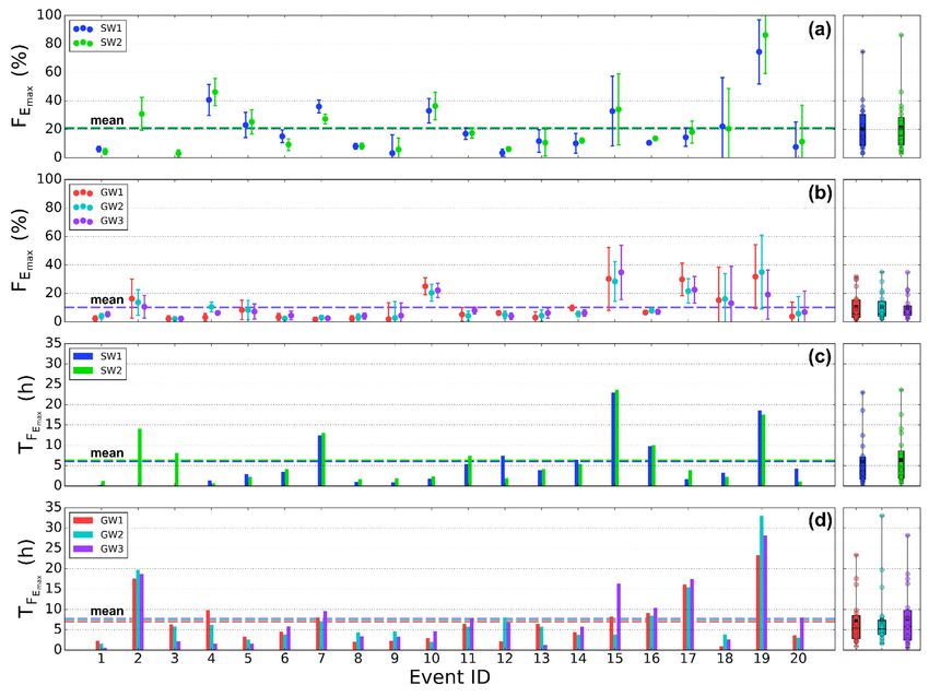
Water 2020, 12, 565                                                                               3 of 19

to investigate the hydrological response behavior and the role of controlling factors on the runoff
generation process, we used a new, trailer-based mobile automatic sampling system for high-resolution
water quality analysis. In particular, we studied the following objectives:

I.     Investigation if the short-term response behavior observed in the previous studies in the
       Schwingbach Environmental Observatory (SEO), is reflected in isotopic signatures of stream
       water and groundwater.
II.    Estimation of event-based contribution of event and pre-event water to total runoff.
III.   Quantification of the event-based response time of maximum event water fraction in stream
       water and groundwater.
IV.    Evaluation of the role of precipitation and antecedent wetness conditions as drivers of event and
       pre-event water contribution and response time.

2. Materials and Methods

2.1. Study Area
      The study was conducted in the headwater catchment of the Schwingbach Environmental
Observatory (SEO) in Hesse, Germany (Figure 1a–c). The 1.03 km2 catchment area is covered by 76%
forests, 15% arable land, and 7% meadows, mainly found along the small perennial Schwingbach
stream. The elevation ranges from 310 m in the north to 415 m a.s.l. in the south. The climate is
temperate oceanic (Köppen climate classification), with a mean annual air temperature of 10.1 ◦ C
and total annual precipitation of 452 mm in the year 2018. Our study took place from August 8th to
December 9th in 2018, which was an unusually dry and warm year [18]. Soil types and geology are
similar to the neighboring valley of the Vollnkirchner Bach [16]. Cambisols dominate on forests stands,
whereas Stagnosols are mainly found on arable land. Under the forests, the soil texture is dominated
by silt, fine sand and gravel at 0 to 3 m depths, with low clay content between 0.6 and 3 m depths.
Soils lay on slightly weathered clay shale bedrock. Under meadows and arable land, the soil texture is
rich in silt and fine sand (0–5 m depths) with small amounts of clay and gravel between 0.8 and 5 m
depths. Here, soils developed on greywacke and weathered clay shale.
      An automatic climate station (AQ5, Campbell Scientific Inc., Shepshed, UK) operated with a
CR1000 data logger measured precipitation depth and air temperature at 5 min intervals. Groundwater
(GW) table depth was manually measured biweekly to obtain an estimate of the groundwater depth
in the unconfined aquifer over the year. The mean groundwater table depth (i.e., mean of biweekly
measurements) from November 2017 to September 2018 was 0.44 ± 0.33 m (mean ± standard deviation),
0.48 ± 0.33 m and 1.41 ± 0.48 m for GW1, GW2, and GW3, respectively. A stream gauge at SW2 (RBC
flume, Eijkelkamp Agrisearch Equipment, Giesbeek, Netherlands) equipped with a pressure transducer
(Micro-Diver, Eigenbrodt Inc., Königsmoor, Germany) automatically recorded water levels at 10 min
intervals. The transducer readings were calibrated against manual measurements and continuous
discharge was derived through the calibrated stage-discharge relationship of the RBC flume provided
by the manufacturer [19]. The discharge was converted to mm h−1 (i.e., divided by the area of the
catchment) to allow for a direct comparison with precipitation in the same unit. Two remote telemetry
loggers (A753, Adcon, Klosterneuburg, Austria), one installed at the toeslope (ST) and one at the
footslope (SF), were equipped with sensors (ECH2O 5TE, METER Environment, Pullman, USA) to
measure soil moisture at 5, 30, and 70 cm soil depths, representing the densely rooted organic horizon,
the topsoil, and subsoil, at 5 min intervals.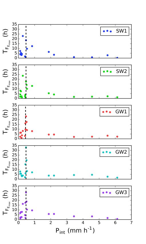
Water 2020, 12,
Water 2020, 12, 565
x FOR PEER REVIEW 21
4 of 19
Figure 1. (a) Schwingbach Environmental Observatory (SEO), (b) Study area in the Schwingbach
Figure 1. (a) Schwingbach Environmental Observatory (SEO), (b) Study area in the Schwingbach
headwater and (c) Measuring network along the stream reach of the Schwingbach headwater. ST and
headwater and (c) Measuring network along the stream reach of the Schwingbach headwater. ST and
SF are the soil moisture stations at the toeslope and footslope, respectively.
SF are the soil moisture stations at the toeslope and footslope, respectively.
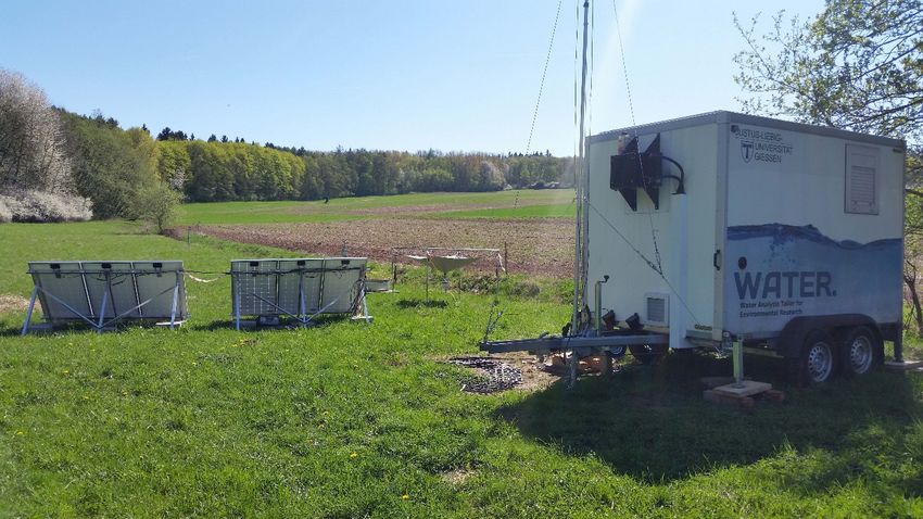
2.2. Water Analysis Trailer for Environmental Research (WATER)
An automatic climate station (AQ5, Campbell Scientific Inc., Shepshed, UK) operated with a
A custom-made, automated mobile laboratory, the Water Analysis Trailer for Environmental
CR1000 data logger measured precipitation depth and air temperature at 5 min intervals.
Research (WATER), was utilized to automatically sample multiple water sources (e.g., stream water,
Groundwater (GW) table depth was manually measured biweekly to obtain an estimate of the
groundwater, and precipitation) and analyze the stable isotopes of water (δ18 O and δ2 H) and water
groundwater depth in the unconfined aquifer over the year. The mean groundwater table depth (i.e.,
chemistry in situ (Figure 2). Constructing the trailer was based on previous experiences made by
mean of biweekly measurements) from November 2017 to September 2018 was 0.44 ± 0.33 m (mean
Heinz et al. [14] and Mahindawansha et al. [15]. Figure 3 illustrates the technical set up of the WATER.
± standard deviation), 0.48 ± 0.33 m and 1.41 ± 0.48 m for GW1, GW2, and GW3, respectively. A stream
The automatic sampling system allows us to sample up to 12 water sources. A peristaltic pump (M1500,
gauge at SW2 (RBC flume, Eijkelkamp Agrisearch Equipment, Giesbeek, Netherlands) equipped with
Verder GmbH, Haan, Germany) draws water from the sources and delivers it through a 5 µm polyester
a pressure transducer (Micro-Diver, Eigenbrodt Inc., Königsmoor, Germany) automatically recorded
membrane (polyester filter, Pieper Filter GmbH, Germany) to a 1000 mL sample reservoir, which is
water levels at 10 min intervals. The transducer readings were calibrated against manual
connected to a continuous water sampler (CWS) (A0217, Picarro Inc., Santa Clara, USA), coupled to a
measurements and continuous discharge was derived through the calibrated stage-discharge
wavelength-scanned cavity ring-down spectrometer (WS-CRDS) (L2130-i, Picarro Inc., Santa Clara,
relationship of the RBC flume provided by the manufacturer [19]. The discharge was converted to
USA) −1to analyze the water’s isotopic composition. The deployment of the Picarro A0217 and L2130-i
mm h (i.e., divided by the area of the catchment) to allow for a direct comparison with precipitation
requires the supply of at least two standard water samples with a known isotopic signature. We used
in the same unit. Two remote telemetry loggers (A753, Adcon, Klosterneuburg, Austria), one installed
heavy (+3.13% for δ18 O and −1.52% for δ2 H) and light (−22.43% for δ18 O and −164.60% for δ2 H)
at the toeslope (ST) and one at the footslope (SF), were equipped with sensors (ECH2O 5TE, METER
standard water samples, which were calibrated via a WS-CRDS (precision of 0.02% for δ18 O and
Environment, Pullman, USA) to measure soil moisture at 5, 30, and 70 cm soil depths, representing
0.18% for δ2 H) at the laboratory of the Institute for Landscape Ecology and Resources Management
the densely rooted organic horizon, the topsoil, and subsoil, at 5 min intervals.
at the Justus Liebig University Giessen, Germany. To prevent the isotope analyzer from falling dry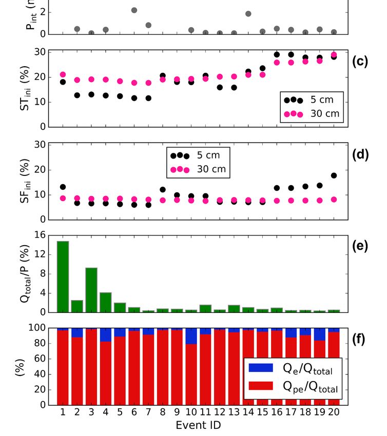
reservoir, which is connected to a continuous water sampler (CWS) (A0217, Picarro Inc., Santa Clara,
   USA), coupled to a wavelength-scanned cavity ring-down spectrometer (WS-CRDS) (L2130-i, Picarro
   Inc., Santa Clara, USA) to analyze the water’s isotopic composition. The deployment of the Picarro
   A0217 and L2130-i requires the supply of at least two standard water samples with a known isotopic
   signature.
Water             We used heavy (+3.13‰ for δ18O and −1.52‰ for δ2H) and light (−22.43‰ for δ18O and
       2020, 12, 565                                                                                                5 of 19
   −164.60‰ for δ2H) standard water samples, which were calibrated via a WS-CRDS (precision of
   0.02‰ for δ18O and 0.18‰ for δ2H) at the laboratory of the Institute for Landscape Ecology and
between
   Resources switching     the samples,
                  Management               a backup
                                   at the Justus      reservoir
                                                  Liebig         is installed.
                                                         University   Giessen,AGermany.
                                                                                  10 L bucket   filled with
                                                                                             To prevent   the deionized
                                                                                                               isotope
water   flushes
   analyzer        the falling
                from    systemdrybetween
                                     betweenthe switching
                                                sampling cycles.    A 5 L abucket
                                                           the samples,           filled
                                                                             backup       by precipitation
                                                                                      reservoir is installed.falling
                                                                                                               A 10 onL a
   bucket filled
funnel-type             2
                 3.3 with
                      m tarpdeionized    water flushes
                                is connected            the system
                                                to the WATER         between the
                                                                for automatic      sampling
                                                                                 sampling      cycles.2).
                                                                                             (Figure   A The
                                                                                                           5 L bucket
                                                                                                                bucket is
   filled bywith
equipped       precipitation    fallingelectrode,
                     a sensor (tank      on a funnel-type
                                                  Votronic3.3 m2 tarp
                                                            GmbH,       is connected
                                                                     Lauterbach,       to the WATER
                                                                                   Germany)            for automatic
                                                                                               to monitor    the amount
of sampling
   the collected  (Figure   2). The bucket
                      precipitation            is equipped
                                       inside the  bucket. with a sensor (tank electrode, Votronic GmbH,
   Lauterbach, Germany) to monitor the amount of the collected precipitation inside the bucket.

      Figure
         Figure2. 2.Water
                     WaterAnalysis
                             Analysis Trailer
                                        Trailer for
                                                 for Environmental  Research(WATER)
                                                     Environmental Research     (WATER)(right),
                                                                                            (right),two
                                                                                                      twosolar
                                                                                                           solar panels
                                                                                                               panels
      supporting
         supporting power supply (left) and the funnel-type tarp for collection of precipitation (further back in
                    power   supply   (left) and  the funnel-type tarp for collection of  precipitation  (further back
      theinmiddle)   installed
            the middle)        in the
                          installed in Schwingbach
                                       the Schwingbach Environmental
                                                          EnvironmentalObservatory
                                                                          Observatory(SEO),
                                                                                        (SEO),Hesse
                                                                                               Hesse(Germany).
                                                                                                       (Germany).

     The WS-CRDS measured the isotopic composition of water vapor every 1.7 s. Due to the carry-over
effects within the CWS, it took approximately 10 min until a steady isotope signal was reached. We
averaged the last 3 min of the following 10 min sampling period to report the final isotope values.
The overall sampling interval per sample summed up to 20 min. To minimize the carry-over effect,
the sample reservoir was automatically rinsed with 60 mL sample water, emptied and again filled
with 60 mL water to be analyzed. Results are reported in (%) for δ18 O and δ2 H relative to the Vienna
Standard Mean Ocean Water (VSMOW).
     Further analytical instruments of the WATER (Figure 3) measure water quality parameters such
as electrical conductivity, pH, and water temperature (via multi-parameter water quality probe,
YSI600R, YSI Inc., Yellow Springs, USA) and NO3 , DOC, TOC, and total suspended sediments via UV
spectrometry (ProPS, Trios GmbH, Rastede, Germany). Results from water quality analysis are not
reported in this study.
     An in-house developed software written in Python runs on an industry PC (NISE 101, SEPCTRA,
Reutlingen, Germany) with the Ubuntu Mate operation system to control the sampling scheme and
the delivery system, as well as to store results and communicate with the WATER. The measurement
processes are controlled by a programmable logic controller (WAGO-I/O-SYSTEM 750, WAGO
Kontakttechnik GmbH, Minden, Germany). Raw data is stored every 5 min and automatically uploaded
to a web-database for visualization, post-processing, and storage. Alarm messages (e.g., a low fuel
gauge or system failure) are automatically triggered by SMS. A diesel backup-generator (with 5 kW
peak), a Lithium-ion buffer battery (7.2 kWh), and two solar panels (with 1.7 kW peak) (Figure 2)
supply the AC and DC power of the system and allow the system to support a continuous load of
approximately 400 W.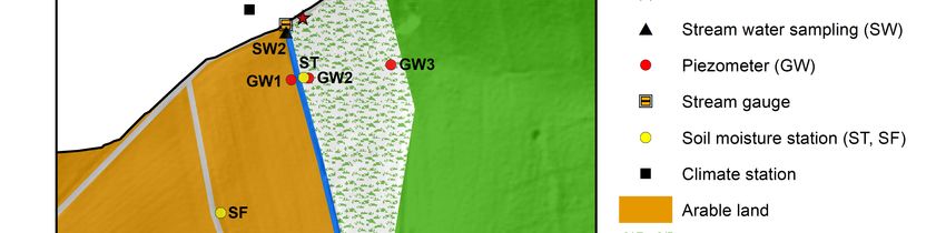
Water 2020, 12, 565 6 of 19
Water 2020, 12, x FOR PEER REVIEW 6 of 21
Figure 3. Schematic
Figure 3. Schematic of the
the sampling
sampling board
board and
and analytical
analytical instrumentation
instrumentation inside the Water
Water Analysis
Analysis
Trailer for Environmental Research (WATER). CWS = continuous water sampler, WS-CRDS ==
Trailer for Environmental Research (WATER). CWS = continuous water sampler, WS-CRDS
wavelength-scanned
wavelength-scannedcavity
cavityring-down
ring-downspectrometer.
spectrometer.
2.3. Sampling Schedule
The WS-CRDS measured the isotopic composition of water vapor every 1.7 s. Due to the carry-
overIn effects within
the setup ofthe
thisCWS, it took
project, approximately
the WATER sampled 10 automatically
min until a steady fromisotope signalwater
two stream was reached.
sources
We averaged
(SW1 and SW2), the three
last 3 min of the following
groundwater sources10(GW1,
min sampling
GW2 and period
GW3), to report
and one theprecipitation
final isotope bucket
values.
The overall
(Figures sampling
1c and 2). SW1 interval per sample
was sampled summed up145
approximately to 20
m min. To minimize
upstream the carry-over
of the WATER effect,
at the edge of
the sample
arable land andreservoir
waterwasfromautomatically
SW2 was taken rinsed
next with
to the60location
mL sampleof thewater,
WATER. emptied
Shallowand again filled
groundwater
withsampled
was 60 mL water fromtopiezometers
be analyzed.madeResultsfromareperforated
reported inPVC (‰)tubes
for δ18sealed
O andwithδ2H relative
bentoniteto the
clayVienna
at the
Standard Mean Ocean Water (VSMOW).
upper part of the tube to prevent contamination by surface water. Piezometers of GW1 and GW2 were
locatedFurther
at theanalytical
toeslope instruments
on arable land of the
andWATER (Figurerespectively.
the meadow, 3) measure water quality parameters
The piezometer of GW3 such
was
as electrical
installed at the conductivity,
footslope at pH, and of
the edge water temperature (via multi-parameter water quality probe,
the forest.
YSI600R,
GivenYSI theInc., Yellowresolution
sampling Springs, USA)
of 20 and
min,NO
the3,setup
DOC,ofTOC, and total
the system suspended
allowed sediments via
the measurement ofUV
72
spectrometry
samples per day. (ProPS, Trios GmbH,
The sampling cycleRastede, Germany).
was scheduled Results
to sample n =from watern quality
16 (with the numberanalysis are not
of samples)
reported
for study.source, n = 8 for each groundwater source and n = 8 for each standard water
in this water
each stream
sample Aninin-house
case of no developed software
precipitation event.written
In thein Python
case runs on an industry
of a precipitation event, thePCsampler
(NISE 101, SEPCTRA,
automatically
Reutlingen,
took Germany)
a precipitation withwhenever
sample the Ubuntu Mate operation
the sample system to1 L
volume exceeded control
(0.3 mm)theinside
sampling scheme and
the precipitation
the delivery
bucket. Aftersystem, as well
sampling, theas to store results
precipitation and communicate
bucket was emptied to with the WATER.
avoid carry-over The measurement
effects, and the
processes
sampler was areblocked
controlled
for 60bymin,
a programmable
allowing us to takelogicsamples
controllerfrom(WAGO-I/O-SYSTEM
other sources. 750, WAGO
Kontakttechnik GmbH, Minden, Germany). Raw data is stored every 5 min and automatically
2.4. Event Definition
uploaded and Characteristics
to a web-database for visualization, post-processing, and storage. Alarm messages (e.g., a
low Wefuelanalyzed
gauge orautocorrelation
system failure)for aretime
automatically triggered by
series of precipitation SMS.measured
depth A diesel over
backup-generator
the sampling
(with 5 kW peak), a Lithium-ion buffer battery (7.2 kWh), and two solar
period to define independent precipitation events [20,21]. A plot of the correlation coefficient panels (with 1.7 kW peak)
with
(Figureto
respect 2) the
supply the AC
lag time and DCthe
indicated power
minimumof thelag
system
time,andfor allow
whichthe thesystem to support
autocorrelation a continuous
coefficient was
load of approximately 400 W.
close to zero. This lag time defined the minimum inter-event time, at which the precipitation events
were considered independent. The autocorrelation plot for the precipitation depth at 5 min intervals
2.3. Sampling
(Figure Schedule
4) shows that correlation coefficients begin to level off close to zero at 5.7 h. We, therefore,
In the setup of this project, the WATER sampled automatically from two stream water sources
(SW1 and SW2), three groundwater sources (GW1, GW2 and GW3), and one precipitation bucket
We analyzed autocorrelation for time series of precipitation depth measured over the sampling
    period to define independent precipitation events [20,21]. A plot of the correlation coefficient with
    respect to the lag time indicated the minimum lag time, for which the autocorrelation coefficient was
    close to zero. This lag time defined the minimum inter-event time, at which the precipitation events
    were
Water  2020,considered
             12, 565      independent. The autocorrelation plot for the precipitation depth at 5 min intervals
                                                                                                             7 of 19
    (Figure 4) shows that correlation coefficients begin to level off close to zero at 5.7 h. We, therefore,
    considered precipitation events as independent if the inter-event time exceeded 6 h. In total, 20 events
considered precipitation events as independent if the inter-event time exceeded 6 h. In total, 20 events
    were selected, at which the application of hydrograph separation was possible due to the availability
were selected, at which the application of hydrograph separation was possible due to the availability
    of isotope concentration data of precipitation, stream water, and groundwater. The beginning of an
of isotope concentration data of precipitation, stream water, and groundwater. The beginning of an
    event was defined as the onset of precipitation and the end of an event as the time whenQe                  ≤ 0.05
event was defined as the onset of precipitation and the end of an event as the time when Qe i ≤ 0.05
                                                                                                        max
    (i.e.,
(i.e., whenwhen
              thethe    fraction
                    fraction     of event
                             of event     water
                                      water       relative
                                             relative to itsto its maximum
                                                             maximum   valuevalue reached
                                                                            reached  5% or 5%
                                                                                           less)ororless)
                                                                                                     when orawhen
                                                                                                              new a
    newbegan,
event      event whichever
                   began, whichever
                               happenedhappened
                                          first. first.

     Figure 4. Autocorrelation plot for the precipitation depth at 5 min intervals. The precipitation events
        Figure 4. Autocorrelation plot for the precipitation depth at 5 min intervals. The precipitation events
     were considered independent if the inter-event time exceeded 6 h.
        were considered independent if the inter-event time exceeded 6 h.
     We calculated a number of hydrometrics to describe precipitation, antecedent wetness,
and response characteristics of each event (Table 1). A Spearman rank correlation (p) analysis
was used to assess the control of precipitation and antecedent wetness hydrometrics on response
characteristics. The correlation values were considered statistically significant if p < 0.05. We described
strength of the correlation strong if p ≥ 0.7, moderate if 0.4 < p < 0.7, and weak if p ≤ 0.4.

     Table 1. Hydrometrics to describe precipitation, antecedent wetness, discharge characteristics,
     maximum event water fraction, and response time for each event.

                 Metric                                   Description                              Unit
              Precipitation
                    P                             Total precipitation per event                    mm
                    T                                Precipitation duration                         h
                   Pint                         Mean precipitation intensity   ( TP )            mm h−1
          Antecedent Wetness
                                            Initial discharge: 1 h averaged discharge
                   Qini                                                                          mm h−1
                                                    before onset of precipitation
Water 2020, 12, 565 8 of 19
Table 1. Cont.
Metric Description Unit
Initial soil moisture: 1 h averaged soil
ST5ini , ST30ini , ST70ini moisture before onset of precipitation at the %
toeslope (ST) at 5, 30 and 70 cm soil depths
Initial soil moisture: 1 h averaged soil
SF5ini , SF30ini , SF70ini moisture before onset of precipitation at the %
footslope (SF) at 5, 30 and 70 cm soil depths
Discharge
Qtotal Total discharge volume per event mm
Qe Total event water volume mm
Qpe Total pre-event water volume mm
Qtotal
P
Runoff coefficient %
Qe
Qtotal
Event water fraction in total runoff %
Qpe
Qtotal
Pre-event water fraction in total runoff %
FEmax Maximum event water fraction %
Response time: time lag between the first
TFEmax detection of precipitation and the maximum h
event water fraction
2.5. Response Characteristics
A two-component hydrograph separation (Equation (1)) was applied to quantify event-water
fractions FE in stream water and groundwater sources using isotopic composition of stream water,
groundwater, and precipitation:
CSW/GW − Cpe
FE = (1)
Ce − Cpe
CSW/GW , Ce and Cpe are the isotopic concentrations in the sampling sources (i.e., stream water SW and
groundwater GW), event water (e) (i.e., precipitation) and pre-event (pe) water of sampling sources,
respectively. Cpe was calculated as the average of the last five samples before the onset of precipitation.
Ce is the incremental weighted mean of precipitation samples [22]. The maximum event water fractions
FEmax in stream water and groundwater were derived for each event at the time steps that resulted from
the sampling schedule. The uncertainty of the event water fractions WFE was quantified according to
the Gaussian error propagation technique [23] (Equation (2)):
2 2 1
2 2
C − C C − C
−1
pe
SW/GW
e
SW/GW
WFE = WCpe + 2 WCe +
WCSW/GW (2)
Ce − Cpe 2
Ce − Cpe
Ce − Cpe
WCpe , the uncertainty in pre-event water was estimated using the standard deviation of the last five
measurements before the onset of precipitation. WCe , the uncertainty of the event water is the standard
deviation of the incremental weighted mean of precipitation. WCSW/GW , the uncertainty in the sampling
sources is the measurement precision of the CWS coupled to the WS-CRDS (0.23% for δ18 O and 0.57%
for δ2 H), which we derived from the standard deviation of measurements during the last 3 min of the
sampling period of stream water and groundwater sources. The uncertainty of event water fractions
was higher using δ18 O measurements than those of δ2 H. Therefore, we performed an analysis based
on the δ2 H values only.Water 2020, 12, 565 9 of 19
We estimated the response time of the maximum event water fraction TFEmax in stream water and
groundwater sources for each event. The response time was defined as the time lag between the first
detection of precipitation and maximum event water fraction.
Total event water volume Qe (Equation (3)) and total pre-event water volume Qpe (Equation (4)) of
each event were calculated from the event water fraction and discharge at each time step i (hourly) as:
X
Qe = FEi × Qi (3)
X
Qpe = Qi − Qei (4)
where FEi , Qi and Qei are the event water fraction in the stream water, the discharge recorded at the
stream gauging site and the event water volume at time step i, respectively. In this study, we estimated
Qei only for SW2 as stream discharge was only recorded at this site. Event water fractions FE were
interpolated linearly with respect to time step i. FE values were also interpolated linearly between the
measurement gaps that happened due to system maintenance. Following, the event water fraction
Q Qpe Qtotal
in total runoff Q e , pre-event water fraction in total runoff Qtotal and the runoff coefficient P were
total
calculated for each event.
3. Results
3.1. Time Series of Isotopic and Hydrometric Observations
The dynamics of precipitation, discharge, soil moisture as well as the δ2 H of precipitation,
stream water, and groundwater sources from August 8th to December 9th in 2018 are shown
in Figure 5a–e. Over the sampling period, precipitation ranged between 0.01 and 3.71 mm h−1 ,
and discharge between 0.0002 and 0.004 mm h−1 with the highest peak at event #19. The discharge
time series shows some distinct peaks, whereas diurnal variations in discharge resulted in a rather
flickering behavior of the hydrograph. The discharge response pattern to precipitation during the
sampling period partly matches the shallow soil moisture development at the toeslope and footslope.
Measured soil moisture indicated generally wetter conditions at all three soil depths at the toeslope
compared to the one at the footslope. Further, the temporal dynamics at the toeslope were also more
pronounced, particularly at 5 cm soil depth. At both sites, the lowest soil moistures were recorded in
late summer at 5 cm soil depth.
The values of δ2 H in precipitation ranged from −10.7% to −108.6% with high within-storm
event variation. From the beginning of the sampling period until early November, the values of δ2 H
in precipitation were heavier than those in stream water and groundwater, whereas they became
significantly lighter over the remaining sampling period. Isotopic concentrations in stream water and
groundwater (i.e., CSW/GW ) as well as in precipitation (i.e., Ce ) were heavier than those in pre-event
water (i.e., Cpe ) until event 15, whereas they became lighter thereafter. Over the entire sampling period,
stream water and groundwater isotopes were almost stable. The mean values of δ2 H for the stream
sampling positions SW1 and SW2 were −63.3 ± 2.1% (mean ± standard deviation) and −63.2 ± 1.7%,
respectively. On average, GW1 (−61.5 ± 1.2%) and GW2 (−61.8 ± 1.3%) at the toeslope depicted
slightly heavier mean δ2 H values compared to the GW3 at the footslope (−63.3 ± 1.2%). Distinct
responses to precipitation were observed in stream water as well as groundwater during events #10,
#17, and #19. However, different response behaviors were found during events #4 and #7, at which
stream water isotopes showed clear responses to precipitation, whereas a slight reaction could be
observed in the groundwater isotopes.Water 2020, 12, x FOR PEER REVIEW 10 of 21
Water 2020, 12, 565 10 of 19
Figure 5. Time series of (a) precipitation and discharge, (b) soil moisture measured at 5, 30 and 70 cm
depths at the toeslope and footslope, (c) δ2 H in precipitation, (d) δ2 H in stream water sources and (e)
Figure 5. Time series of (a) precipitation and discharge, (b) soil moisture measured at 5, 30 and 70 cm
δ2 H in groundwater water sources. The vertical grey bars indicate the 20 events. The numbers on top
depths at the toeslope and footslope, (c) δ2H in precipitation, (d) δ2H in stream water sources and (e)
of2 panel (a) represent the event ID.
δ H in groundwater water sources. The vertical grey bars indicate the 20 events. The numbers on top
of panel (a) represent the event ID.
3.2. Hydrometrics
Hydrometrics
The values of δ2of precipitation,
H in precipitationantecedent
ranged fromwetness,
−10.7‰and discharge
to −108.6‰ characteristics,
with as well
high within-storm as
event
maximum event water fraction, its uncertainty and response time of stream water and groundwater
variation. From the beginning of the sampling period until early November, the values of δ H in 2
precipitation were heavier than those in stream water and groundwater, whereas they becameWater 2020, 12, 565 11 of 19
sources, were calculated for each of the 20 events (Tables S1–S3 in the Supplementary Materials).
Figure 6a–f shows the variation of the total precipitation, mean precipitation intensity, initial soil
moisture in shallower layers (i.e., 5 and 30 cm) at the toeslope and footslope, runoff coefficient,
and event and pre-event water fraction in the total runoff for the 20 events. Total precipitation P ranged
between 0.3 and 19.6 mm (3.2 ± 5.2 mm, mean ± standard deviation). The largest total precipitation
was observed at event #19 followed by event #7 (Figure 6a). Mean precipitation intensity Pint ranged
between 0.1 and 6.1 mm h−1 (1.4 ± 1.9 mm h−1 ). Larger Pint was observed among the first nine events,
with the largest value at event #1, followed by event #5 and #9 (Figure 6b).
Water 2020, 12, x FOR PEER REVIEW 12 of 21
Figure (a)(a)Total
6. 6.
Figure Totalprecipitation
precipitation per event P,
perevent (b)
, (b) mean
mean rainfall
rainfall intensity, P(c)
intensity , (c) initial
intinitial soil moisture
soil moisture
at the toeslope ST in 5 and 30
at the toeslope in 5 and 30 cm depths, (d) initial soil moisture at the footslope SF in 5
depths, (d) initial soil moisture at the footslope in 5 and 30and
cm 30 cm
depths, Q Q Qpe
depths, (e) (e) runoff
runoff coefficient P
and
coefficient total and (f)(f) event
event water
water fraction e and
fraction Qtotal
andpre-event
pre-eventwater
waterfraction
fraction
Qtotal of
the 20 precipitation events. events.
of the 20 precipitation
Initial soil moisture at the toeslope position showed an increasing trend over the sampling
events at both, 5 and 30 cm soil depths (Figure 6c). 5 values were lower than those in 30
until event #7, and subsequently reached slightly higher values over the last events. By contrast, the
initial soil moisture at the footslope was quite stable with a slight decrease over the sampling eventsWater 2020, 12, 565 12 of 19
Initial soil moisture at the toeslope position showed an increasing trend over the sampling events
at both, 5 and 30 cm soil depths (Figure 6c). ST5ini values were lower than those in ST30ini until event
#7, and subsequently reached slightly higher values over the last events. By contrast, the initial soil
moisture at the footslope was quite stable with a slight decrease over the sampling events at 30 cm
depth, whereas an increasing trend with variation in between was observed at 5 cm depth (Figure 6d).
The runoff coefficient was relatively low, less than 2% for most of the events and with a mean
of 2.2 ± 3.5% (Figure 6e). The highest runoff coefficient amounted to 14.8% at event #1, with a total
precipitation input of only 1 mm but with a relatively high SF5ini of around 13%. The overall trend of
runoff coefficient across the events showed that the events with relatively higher total precipitation did
not necessarily result in higher rainfall-runoff ratios. Very low runoff coefficients (Water 2020, 12, 565 13 of 19
Water 2020, 12, x FOR PEER REVIEW 14 of 21
(a,b) Maximum
Figure 7. Figure event
7. (a,b) Maximum water
event fraction FEmax for
waterfraction forstream
stream water
water (SW) (SW) and groundwater
and groundwater (GW) (GW)
sources, including the uncertainty
sources, including of estimations
the uncertainty (error
of estimations bars)
(error bars)and
and (c,d) response
(c,d) response time
time of maximum event
of maximum
event T
water fraction water fraction for the same water sources. SW1 was not sampled at event #2 and #3.
FEmax for the same water sources. SW1 was not sampled at event #2 and #3. Boxplots
Boxplots (right panels) represent the interquartile range, black bars the median, black squares the
(right panels) represent the interquartile range, black bars the median, black squares the mean and the
mean and the whiskers the range of all 20 events.
whiskers the range of all 20 events.
Relatively large uncertainties of maximum event water fraction of 20% and more existed at
3.3. Correlations of Hydrometrics
events #15, #18, #19, and #20 (Figure 7a,b) due to the large temporal variation of isotope values in
precipitation and concurrent small differences between the isotopic composition of event and pre-
In order to investigate the role of precipitation and antecedent wetness conditions on discharge
event water. For the remaining events, the uncertainty was on average roughly 6% and 5% for stream
characteristics, maximum
water and event
groundwater, water fraction and response time, we tested their correlations (Table 2).
respectively.
Event water contribution
The response time increased
of maximum significantly with the precipitation
event water fraction ranged fromamount.
0.3 h to 24 hInand
turn,
0.6 htotal event
Qe
water volumeto 33 Qh einand
stream water
event and groundwater,
water respectively
fraction in total runoff(Figure 7c,d). On average,
correlated the event
positively withwater
precipitation
Qtotal
amount P,fraction
whilst reached
totalitspre-event
maximum after 6 h in
water the stream
volume Qpewater
was(i.e., SW1 and SW2).
strongest Differences
related to the between
initial discharge
in the two stream water sources were small (1.3 h mean absolute difference), except at event
Qini . No significant correlation was found for any of the soil moisture characteristics at the toeslope
#12, #17, and #20, at which the differences were larger than 5 h, 2 h, and 3 h, respectively. In
and discharge characteristics.
comparison, the event water By fractions
contrast,infootslope
groundwater soil
at moisture
the toeslopein(GW1
deeper
and soil
GW2)layers
and the indicated a
significantfootslope
impact(GW3)on totaltookpre-event water
a little longer contribution
to reach their maximaandwiththe7–8runoff coefficient.
h. The longer response times in
the stream
Maximum eventwater (i.e., at
water event #2,F#7, #15,
fraction and #19) as well as in the groundwater (i.e., at event #2, #17,
Emax in the stream water increased with the amount and duration
and #19) were observed at times when was above its mean value.
of precipitation. FEmax in groundwater was also related to the precipitation amount but with a less
strong correlation. Particularly
3.3. Correlations of Hydrometricsnoteworthy was the importance of initial soil moisture conditions at
the toeslope. In order to investigate the role of precipitation and antecedent wetness conditions on discharge
The response times
characteristics, TFEmax of
maximum GW1
event and
water GW3and
fraction correlated moderately
response time, we testedwith total precipitation
their correlations (Table similar
2). Event water contribution increased significantly with the precipitation
to TFEmax of SW1 and GW3 with precipitation duration and initial soil moisture of 70 cm depth at the amount. In turn, total
event water
toeslope (Table 2). No volume and event correlations
other significant water fractionwere
in total runoff
established correlated
for any of the positively with
hydrometrics listed
in Table 1. Nevertheless, we observed a clear two-state system with respect to the mean precipitation
intensity Pint (Figure 8). In the first state, no relationship could be depicted between TFEmax and Pint .
After a certain threshold of Pint , the system swapped into a second state, at which TFEmax decreased
with increasing Pint . In order to identify the threshold, we calculated the Spearman rank correlation
between TFEmax and Pint by leaving out one event after another starting from the event with the lowest
Pint . The Pint where we found the highest Spearman rank correlation coefficient was considered as the
threshold. The Spearman rank correlation coefficients ranged between −0.99 and −0.88 (p < 0.001) forWater 2020, 12, 565 14 of 19
all water sources. The threshold values were 0.47 mm h−1 for SW1, SW2, GW2, and GW3 and 0.44 mm
h−1 for GW1 (Figure 8).
Table 2. Spearman rank correlation coefficients (p) for the relationships of precipitation and antecedent
wetness characteristics with discharge characteristic, maximum event water fraction and its response
time (see Table 1 for acronyms). Green bolded cells represent statistically significant correlations with
p < 0.05.
P T Pint Qini ST5ini ST30ini ST70ini SF5ini SF30ini SF70ini
Qtotal 0.54 0.10 0.33 0.69 −0.39 −0.30 −0.37 −0.38 0.43 0.44
Qe 0.73 0.29 0.23 0.53 −0.36 −0.25 −0.34 −0.25 0.28 0.33
Qpe 0.48 0.05 0.37 0.74 −0.43 −0.36 −0.44 −0.41 0.46 0.45
Qtotal
P
−0.39 −0.53 0.17 0.49 −0.42 −0.39 −0.32 −0.38 0.59 0.48
Qe
Qtotal
0.64 0.41 −0.06 0.05 −0.04 0.02 −0.04 0.04 −0.10 0.00
Qpe
Qtotal
−0.64 −0.41 0.06 −0.05 0.04 −0.02 0.04 −0.04 0.10 0.00
FEmax SW1 0.75 0.58 −0.12 0.25 −0.18 −0.17 −0.10 −0.29 −0.14 0.05
FEmax SW2 0.75 0.56 −0.06 −0.01 0.03 0.01 0.09 −0.07 −0.21 −0.09
FEmax GW1 0.46 0.33 −0.20 −0.27 0.47 0.46 0.50 0.26 −0.42 −0.18
FEmax GW2 0.52 0.44 −0.20 −0.21 0.46 0.48 0.49 0.34 −0.34 −0.07
FEmax GW3 0.45 0.30 −0.17 −0.28 0.50 0.46 0.45 0.36 −0.43 −0.23
TFEmax SW1 0.32 0.69 −0.42 −0.27 0.18 0.24 0.51 −0.15 −0.33 −0.11
TFEmax SW2 0.31 0.34 −0.13 −0.08 0.03 −0.03 0.13 −0.26 −0.23 −0.16
TFEmax GW1 0.53 0.39 −0.11 0.11 0.03 0.02 0.01 −0.16 0.03 0.08
Water 2020, 12, x FOR PEER REVIEW 16 of 21
TFEmax GW2 0.19 0.43 −0.26 −0.01 0.01 −0.03 −0.15 −0.04 −0.13 0.00
TFEmax GW3 0.53 0.45 −0.13 −0.37 0.38 0.23 0.15 0.15 −0.38 −0.33
Figure 8. Response time TFEmax of stream water and groundwater sources versus mean precipitation
Figure 8. Response time of stream water and groundwater sources versus mean precipitation
intensity Pint . The dashed line is the threshold, at which the response time decreased with increasing
intensity . The dashed line is the threshold, at which the response time decreased with increasing
mean precipitation intensity. The threshold
mean precipitation valuevalue
intensity. The threshold waswas0.47 mm
0.47 mm
−1 h−1
h for SW1,for
SW2,SW1, SW2,
GW2, and GW3 andGW2, and GW3 and
−1 0.44 mm h for GW1.
−1
0.44 mm h for GW1.Water 2020, 12, 565 15 of 19
4. Discussion
4.1. The Schwingbach is Highly Responsive to Precipitation
Our findings show that the short-term response behavior observed in the previous studies in
the SEO [16,17], is reflected in the isotopic signatures of stream water and groundwater. The isotopic
responses in stream water and groundwater during the precipitation events often disclosed a rapid
mixing of water in the sampling sources with event water indicating that the Schwingbach is a highly
responsive catchment to incoming precipitation. The results reported that the average response time
was 6 h in stream water and 7 h and 8 h for groundwater at the toeslope and footslope, respectively.
Capturing event-based isotopic variation in stream water and groundwater emphasized the advantage
of high-resolution sampling of multiple sources, giving insight into catchment response and runoff
generation mechanisms. Firstly, the automated high-resolution sampling revealed the fine-scale
hydrological responses of the stream water and groundwater, which could not be captured with
manual isotope sampling in the previous study [17]. Secondly, the high-resolution data constrained
the interpretation of event water contribution derived from hydrograph separation by the continuous
sampling of stream water. Thirdly, sampling of groundwater along the stream water, showed that the
groundwater response times, particularly at the toeslope, were close to the stream water response times.
This underlines the linkage between stream water and shallow subsurface flow and consequently, the
vital role of shallow subsurface flow in runoff generation in the Schwingbach.
4.2. Pre-Event Water Dominates Runoff Generation
Tracer-based hydrograph separations indicated that more than 79% of runoff consisted of pre-event
water. Due to the highly permeable soils, the contribution of overland flow was negligible and hence
precipitation infiltrated to the subsurface and mobilized pre-event water. Similar findings were
reported in previous studies in other catchments, where pre-event water was also the major contributor
to streamflow [7,24–26].
The runoff coefficients we found were very low (mean of 2.2%). Low runoff coefficients are mainly
a result of high soil permeability and dry catchment wetness conditions [27]. The high porosity of the
soils in the upper layers of meadows and arable land (i.e., silty sand), as well as the extremely dry
conditions in summer 2018, were likely reasons for the low runoff coefficients we measured. Other
studies also reported low event runoff coefficients of less than 2% [28,29]. They found that the high
porosity of the soil, lack of anthropogenic effects such as soil compaction and dry antecedent wetness
conditions were the main reasons for low runoff coefficients.
4.3. Shallow Subsurface Flow Pathways Rapidly Deliver Water to the Stream
The short response times of groundwater and stream water suggests the rapid movement of
water vertically in the soil profile and in lateral downslope direction through shallow subsurface
flow pathways. The short response times in the stream water (on average 6 h) as well as in the
groundwater, particularly at the toeslope with on average 7 h, confirmed the linkage between stream
water and shallow subsurface flow pathways. This linkage became likely stronger during events,
at which maximum event water fractions in groundwater were above mean values such as event #10
and #19 (Figure 7a,b), and in turn, increased the event water fraction in total runoff (Figure 6f). Other
studies also identified shallow subsurface as the dominant contributor to runoff generation [5,7,25,30].
Possible flow pathways leading to fast response times in stream water and groundwater can be vertical
and lateral macropore flow pathways through unsaturated or partially saturated soil matrix [31–34].
During the dry summer of 2018, an extended crack network developed that had the potential to act as
a drainage system. Water transmission can be very high through this vertically-oriented continuous
network of macropores, even higher than rainfall intensities [33]. We conclude this to have happened
in our system in view of the short response times we found in the groundwater. Furthermore, the
relatively flat areas at the toeslope and the stream banks likely contributed to the rapid transmission ofWater 2020, 12, 565 16 of 19
water. These areas have the potential to quickly saturate, store water, and rapidly release water to the
stream network even during small precipitation events [35,36]. This assumption was supported by the
distinct response of shallow soil moisture to precipitation events at the toeslope, which was not clearly
visible at the footslope.
4.4. Variable Controls of Runoff Generation
Total event water volume and event water fraction in total runoff correlated positively with total
event precipitation, pointing out that event water contribution increased with the precipitation amount
(Table 2). Our results are consistent with previous studies, which also reported growing event water
contribution with rising precipitation amounts [4,5,7,10]. Higher precipitation amounts led to an
increase of maximum event water fraction, total event water volume, and event water fraction in total
runoff. This suggests that the maximum event water fraction can be considered as a qualitative proxy
to indicate the overall contribution of event water to runoff. The positive correlation of the maximum
event water fraction in groundwater sources with precipitation amount and initial soil moisture at
the toeslope underlined that not only the higher precipitation amount led to an increase of event
water contribution but also that wetter conditions at the toeslope facilitated groundwater recharge
mechanisms to switch on.
Total pre-event volume correlated moderately with total precipitation amount (Table 2) suggesting
that increasing precipitation led to the mobilization of pre-event water. Albeit the rising total pre-event
water volume, the pre-event water fraction in total runoff decreased, indicating the gaining importance
of event water contribution at the same time. Wetter antecedent conditions often lead to an increase
of pre-event water contribution [4,5,7,9,10]. Despite significant correlations of initial discharge and
initial soil moisture of deeper layers at the footslope with total pre-event volume, we did not observe
significant correlations between pre-event water fraction in total runoff and antecedent wetness
hydrometrics in our system. Moreover, for catchments where pre-event water prevails in runoff
generation, it is usually expected that antecedent wetness conditions show a major influence on the
runoff coefficient. Although we detected significant correlations of the runoff coefficient with storm
duration and antecedent wetness conditions in the Schwingbach, correlations were not strong and
in the case of soil moisture conditions at the toeslope, they were even insignificant. This could be
due to the dry and warm weather conditions during the study period, which resulted in only a small
range of antecedent wetness conditions impacting the correlation analysis. Therefore, we conclude that
pre-event water contribution was only moderately affected by precipitation amount, whereas under
extremely dry conditions such as in the year 2018, the antecedent wetness was too low to impact the
pre-event water contribution.
With a closer look at the response time variation with respect to the mean precipitation intensity
(Figure 8), we detected a threshold of mean precipitation intensity, at which the response time behavior
changed. Whereas there was no clear pattern before the threshold, the response times in stream
water and groundwater decreased with increasing mean precipitation intensity after the threshold.
This suggests that an increase in the mean precipitation intensity after a certain precipitation sum
enhanced infiltration and that water rapidly drained causing event water fraction to reach its peak
faster. Surprisingly, this threshold was very low with only 0.5 mm h−1 , from where rainfall intensity
likely controlled the initiation of macropore flow. It underlines that macropore networks governed flow
control beyond the threshold. For mean precipitation intensities lower than the threshold, the trigger
was not strong enough to control the response behavior.
5. Conclusions
Here we reported on high temporal resolution (20-min intervals) measurements of stable isotopes
from groundwater, stream water, and precipitation to investigate the response of runoff components
and the underlying controlling factors of precipitation and antecedent wetness characteristics. TheWater 2020, 12, 565 17 of 19
analysis focused on 20 precipitation events in the Schwingbach Environmental Observatory (SEO)
in Germany.
We conclude that high temporal resolution sampling of multiple sources, especially in systems
with rapid hydrological responses, has a large potential to gain further insight into the runoff generation
process. High temporal resolution sampling uncovered the event-based isotopic variation in stream
water and groundwater and helped to constrain event and pre-event water contribution. The results
of this investigation stress the importance of shallow subsurface flow contribution to the runoff in
headwater systems. The sampling of groundwater in different hillslope positions and under different
land uses increased the spatial resolution and led to better identify the main flow pathways during
rapid delivery of water to the stream. We suggest that further studies be carried out over longer
periods and that different land uses and slopes be taken into account in varying weather conditions.
Supplementary Materials: The following are available online at http://www.mdpi.com/2073-4441/12/2/565/s1,
Table S1: Precipitation, antecedent wetness and discharge characteristics for the 20 events, Table S2: Maximum
event water fraction FEmax , uncertainty of maximum event water fraction WFE and response time TFEmax of stream
water and groundwater sources derived from δ2 H values for the 20 events, Table S3: Maximum event water
fraction FEmax , uncertainty of maximum event water fraction WFE and response time TFEmax of stream water and
groundwater sources derived from δ18 O values for the 20 events.
Author Contributions: Conceptualization, A.S., L.B., P.K., D.W.; methodology, P.K., D.W., A.S.; software, P.K.,
A.S.; validation, A.S., L.B., P.K.; formal analysis, A.S.; investigation, A.S.; resources, A.S., L.B., P.K., D.W.; data
curation, A.S., P.K.; writing—original draft preparation, A.S.; writing—review and editing, L.B., P.K.; visualization,
A.S.; supervision, L.B., P.K.; project administration, L.B.; funding acquisition, L.B. All authors have read and
agreed to the published version of the manuscript.
Funding: This research received no external funding.
Conflicts of Interest: The authors declare no conflict of interest.
References
1. Klaus, J.; McDonnell, J.J. Hydrograph separation using stable isotopes: Review and evaluation. J. Hydrol.
2013, 505, 47–64. [CrossRef]
2. Shanley, J.B.; Kendall, C.; Smith, T.E.; Wolock, D.M.; McDonnell, J.J. Controls on old and new water
contributions to stream flow at some nested catchments in Vermont, USA. Hydrol. Process. 2002, 16, 589–609.
[CrossRef]
3. Šanda, M.; Sedlmaierová, P.; Vitvar, T.; Seidler, C.; Kändler, M.; Jankovec, J.; Kulasová, A.; Paška, F. Pre-event
water contributions and streamwater residence times in different land use settings of the transboundary
mesoscale Lužická Nisa catchment. J. Hydrol. Hydromech. 2017, 65, 154–164. [CrossRef]
4. Pellerin, B.A.; Wollheim, W.M.; Feng, X.; Vörösmarty, C.J. The application of electrical conductivity as a
tracer for hydrograph separation in urban catchments. Hydrol. Process. 2008, 22, 1810–1818. [CrossRef]
5. James, A.L.; Roulet, N.T. Antecedent moisture conditions and catchment morphology as controls on spatial
patterns of runoff generation in small forest catchments. J. Hydrol. 2009, 377, 351–366. [CrossRef]
6. Fischer, B.M.C.; Stähli, M.; Seibert, J. Pre-event water contributions to runoff events of different magnitude in
pre-alpine headwaters. Hydrol. Res. 2017, 48, 28–47. [CrossRef]
7. Von Freyberg, J.; Studer, B.; Rinderer, M.; Kirchner, J.W. Studying catchment storm response using event- and
pre-event-water volumes as fractions of precipitation rather than discharge. Hydrol. Earth Syst. Sci. 2018, 22,
5847–5865. [CrossRef]
8. Renshaw, C.E.; Feng, X.; Sinclair, K.J.; Dums, R.H. The use of stream flow routing for direct channel
precipitation with isotopically-based hydrograph separations: The role of new water in stormflow generation.
J. Hydrol. 2003, 273, 205–216. [CrossRef]
9. Muñoz-Villers, L.E.; McDonnell, J.J. Runoff generation in a steep, tropical montane cloud forest catchment
on permeable volcanic substrate. Water Resour. Res. 2012, 48. [CrossRef]
10. Penna, D.; van Meerveld, H.J.; Oliviero, O.; Zuecco, G.; Assendelft, R.S.; Dalla Fontana, G.; Borga, M. Seasonal
changes in runoff generation in a small forested mountain catchment. Hydrol. Process. 2015, 29, 2027–2042.
[CrossRef]You can also read