Effect of Land Use Changes on Water Quality in an Ephemeral Coastal Plain: Khambhat City, Gujarat, India - MDPI
←
→
Page content transcription
If your browser does not render page correctly, please read the page content below
water
Article
Effect of Land Use Changes on Water Quality in an
Ephemeral Coastal Plain: Khambhat City,
Gujarat, India
Pankaj Kumar 1, * , Rajarshi Dasgupta 1 , Brian Alan Johnson 1 , Chitresh Saraswat 2 ,
Mrittika Basu 3 , Mohamed Kefi 4 and Binaya Kumar Mishra 5
 1   Natural Resources and Ecosystem Services, Institute for Global Environmental Strategies, Hayama,
     Kanagawa 240-0115, Japan; dasgupta@iges.or.jp (R.D.); johnson@iges.or.jp (B.A.J.)
 2   Institute for the Advanced Study of Sustainability, United Nations University, 4-53-70, Jingumae, Shibuya,
     Tokyo 150-8925, Japan; saraswat.chitresh@gmail.com
 3   Laboratory of Landscape Ecology and Planning, The University of Tokyo, Tokyo 150-8925, Japan;
     mrittika.basu@gmail.com
 4   Laboratory of Natural Water Treatment (LabTEN), Water Researches and Technologies Center (CERTE),
     University of Carthage, Carthage 273-8020, Tunisia; moh_kefi@yahoo.fr
 5   Faculty of Science and Technology, Pokhra University, Pokhra 56305, Nepal; mishra_binaya@hotmail.com
 *   Correspondence: kumar@iges.or.jp; Tel.: +81-070-1412-4622

 Received: 8 February 2019; Accepted: 3 April 2019; Published: 8 April 2019

 Abstract: Rapid changes in land use and land cover pattern have exerted an irreversible change on
 different natural resources, and water resources in particular, throughout the world. Khambhat City,
 located in the Western coastal plain of India, is witnessing a rapid expansion of human settlements,
 as well as agricultural and industrial activities. This development has led to a massive increase in
 groundwater use (the only source of potable water in the area), brought about significant changes
 to land management practices (e.g., increased fertilizer use), and resulted in much greater amounts
 of household and industrial waste. To better understand the impacts of this development on the
 local groundwater, this study investigated the relationship between groundwater quality change and
 land use change over the 2001–2011 period; a time during which rapid development occurred. Water
 quality measurements from 66 groundwater sampling wells were analyzed for the years 2001 and 2011,
 and two water quality indicators (NO3 − and Cl− concentration) were mapped and correlated against
 the changes in land use. Our results indicated that the groundwater quality has deteriorated, with
 both nitrate (NO3 − ) and chloride (Cl− ) levels being elevated significantly. Contour maps of NO3 −
 and Cl− were compared with the land use maps for 2001 and 2011, respectively, to identify the impact
 of land use changes on water quality. Zonal statistics suggested that conversion from barren land to
 agricultural land had the most significant negative impact on water quality, demonstrating a positive
 correlation with accelerated levels of both NO3 − and Cl− . The amount of influence of the different
 land use categories on NO3 − increase was, in order, agriculture > bare land > lake > marshland >
 built-up > river. Whereas, for higher concentration of Cl− in the groundwater, the order of influence
 of the different land use categories was marshland > built-up > agriculture > bare land > lake > river.
 This study will help policy planners and decision makers to understand the trend of groundwater
 development and hence to take timely mitigation measures for its sustainable management.

 Keywords: groundwater; water pollution; land use change; sustainable water management

Water 2019, 11, 724; doi:10.3390/w11040724                                         www.mdpi.com/journal/water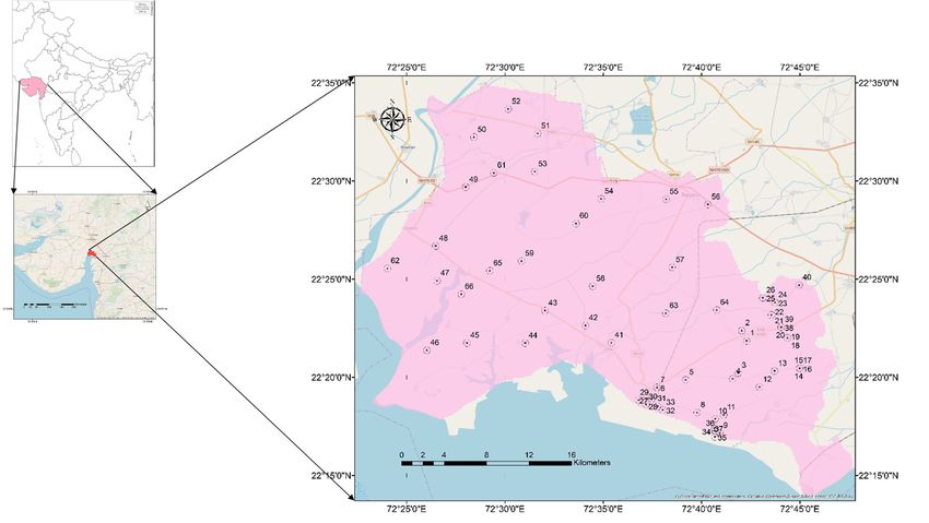
Water 2019, 11, 724                                                                                  2 of 15

1. Introduction
      In many regions, already-scarce freshwater resources are under an unprecedented amount of
stress from different drivers and pressures, including urbanization, land use change, population
growth, increased food/water demand, and climate change [1,2]. It has been well reported that the
cumulative effects of both natural and anthropogenic activities have significant impacts on land use,
which ultimately affects the services provided by the local ecosystems (e.g., their ability to provision
and regulate fresh surface water and groundwater) [3,4]. This is exacerbated by the lack of water
governance and inadequate infrastructure in many developing countries [5,6]. Recognizing this
problem, the United Nations Sustainable Development Goals (SDGs) highlights the necessity of clean
water for achieving different goals pertaining to environmental (e.g., Goal 14, Life below water) and
human well-being (e.g., Goal 6, Clean water and sanitation; and Goal 2, Zero hunger) [7]. Also along
these lines, a recent study found that more holistic and integrated land use management practices
could help achieve SDGs related to water, food, health, and climate change [8]. Water governance has
an important role to play in this kind of holistic/integrated land use management.
      Water governance is also a particularly important issue when it comes to coastal aquifer systems
because of their vulnerability to salt water intrusion. More than sixty percent of the global population
is living in coastal regions or low-lying deltaic zones, so it is imperative to monitor the effects of
different factors affecting water quality in coastal plains [9]. Furthermore, because of the limited
amount of freshwater resources in many coastal areas, it is essential to change water consumption
patterns to achieve a stable hydrodynamic state in future [10,11]. Among different groundwater
quality parameters, nitrate is particularly significant because of its great leachability in soils and its
significant connection with fertilizer use, as well as with inadequate domestic/industrial wastewater
treatment [12,13]. Long-term consumption of water with nitrate concentrations exceeding the
permissible limit (>45 mg/L) set by [14,15] can lead to low oxygen levels in the blood of infants,
a life-threatening situation also known as methemoglobinemia [16]. In addition to nitrate, chloride is
another important groundwater quality parameter that is sensitive to land use and land management
practices, especially in coastal zones due to seawater intrusion [17,18]. When groundwater levels are
reduced in coastal areas (e.g., due to drought or excessive groundwater pumping), salt water with high
levels of chloride can infiltrate into the groundwater aquifer. The main reason behind this is inland
movement of sea water- fresh water interface and approaching the well screen. Although the health
effects of consuming groundwater with levels of high chloride are not well reported, this degraded
groundwater is less suitable for other important purposes (e.g., crop irrigation).
      Several scientific works have used different analysis techniques, including regression modeling,
time series analysis, and geospatial modeling (e.g., using remote sensing and geographical information
systems), to identify the spatio-temporal relationships between groundwater quality changes and
different anthropogenic activities [19–24]. With the above background, it is of utmost importance to
understand the relationship between land use changes and water quality in developing countries like
India with burgeoning populations. This kind of analysis not only helps to identify possible threats to
water quality, but also provides vital information to decision makers to allow them to take adaptive
measures to ensure sustainable water development. This work strives to quantify the effect of land use
changes from 2001 to 2011 on groundwater quality of Khambhat city, a coastal city located in the Gujarat
state, Western India. Khambhat was selected as our study site due to the rapid changes in groundwater
development and land use practices witnessed there in recent years, along with the absence of guidance
and regulations for its sustainable management. In addition, water bodies in the area have recently
experienced algal blooms [25] and salt water intrusion [26]. In this study, nitrate is used as an indicator
to trace the link between land use changes and groundwater quality changes because of its high
solubility, while chloride is used to evaluate the effect of increased groundwater use and its impact
on groundwater salinization. Our evaluation is based on an integrated predictive physically based
modeling system (spatial interpolation and zonal statistics) of groundwater–agriculture–urbanization.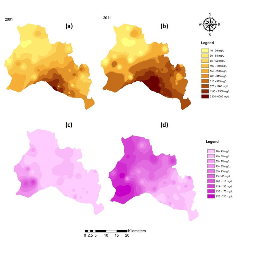
Water 2019, 11, 724 3 of 15
In addition, different management policies are proposed as adaptive measures to minimize further
deterioration
Water 2019, 11, of groundwater
x FOR quality.
PEER REVIEW 3 of 17
2.2.Study
StudyArea
Area
Khambhat,
Khambhat,formerly
formerlyknown knownasasCambay,
Cambay, is is
a city
a city located
located ininthe Anand
the Anand district ofofthe
district theIndian
Indianstate
state
ofofGujarat (Figure 1). It lies on a sedimentary plain at the north end of the
Gujarat (Figure 1). It lies on a sedimentary plain at the north end of the Gulf of Khambhat, which Gulf of Khambhat, which is
noted for the
is noted for extreme
the extreme rise and
rise fall
andoffall
itsof
tides, ranging
its tides, by as by
ranging much as 9.1 as
as much m (the highest(the
9.1 meters in the world)
highest in in
the
the vicinity
world) of Khambhat.
in the vicinity of The averageThe
Khambhat. elevation
average of elevation
the area isof8 them above
area ismean sea level.
8 meters aboveThe meanmain sea
alluvial sediment
level. The formation
main alluvial is of theformation
sediment quaternary age,
is of theand principally
quaternary age,deposited by the Mahi
and principally River;
deposited by
therefore,
the Mahithe soil is
River; highly fertile.
therefore, the soilThe area to fertile.
is highly the south Theofarea
Khambhat consists
to the south of muddy wetlands
of Khambhat consists of
following along the following
muddy wetlands coastline. The along climate is warm The
the coastline. and humid,
climate withis warman annual average
and humid, temperature
with an annual
ofaverage◦
27.4 C temperature
and an average rainfall of 739
of 27.4 °C and anmm/year, most ofofwhich
average rainfall is received
739 mm/year, during
most the south-west
of which is received
monsoon
during the between June and
south-west September.
monsoon betweenMonthlyJune average rainfall and
and September. temperature
Monthly average forrainfall
both year and
2001 and year 2011 are shown in Figure 2, which indicates that there are
temperature for both year 2001 and year 2011 are shown in Figure 2, which indicates that there are no significant changes (data
procured from Indian
no significant changes Meteorological
(data procuredDepartment
from Indianweb portal). The average
Meteorological groundwater
Department web level is 6–8 The
portal). m
below
averageground [27]. As oflevel
groundwater the 2011
is 6–8census,
metersKhambhat
below ground had a[27].
population
As of the of 2011
99,114 (census,
census, 2011), which
Khambhat had a
was 80,439 in of
population year 2001(census,
99,114 with a growth rate of was
2011), which 4.1%80,439
per year. However,
in year in the
2001 with a recent
growthpast,rate Khambhat
of 4.1% per
city hasHowever,
year. witnessedindrastic population
the recent growth, rapid
past, Khambhat city urbanization
has witnessed and sizable
drastic growth ingrowth,
population agricultural
rapid
activity becauseand
urbanization of the highgrowth
sizable fertilityinofagricultural
the land. These activity factors
becausehaveofledthetohigh
a significant
fertility ofchange in land
the land. These
use, which
factors is still
have led continuing.
to a significant change in land use, which is still continuing.
Figure 1. Study area map with sampling locations.
Figure 1. Study area map with sampling locations.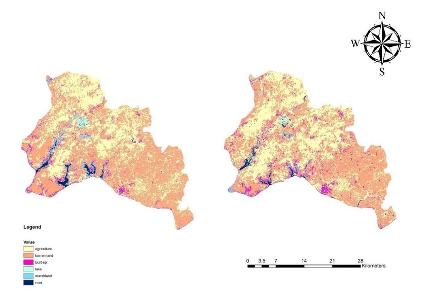
Water
Water 2019,
      2019, 11,
            11, x724
                  FOR PEER REVIEW                                                                                                    4 4ofof17
                                                                                                                                             15

                           300                                                                                                  35

                           250                                                                                                  30
   Monthly rainfall (mm)

                                                                                                                                25

                                                                                                                                       Temperature (°C)
                           200
                                                                                                                                20
                           150
                                          Avg. rainfall (2001)
                                          Avg. rainfall (2011)                                                                  15
                           100            Avg. temp. (2001)
                                          Avg. temp. (2011)                                                                     10

                            50                                                                                                  5

                             0                                                                                                  0
                                 Jan Feb Mar Apr May Jun Jul Aug Sep Oct Nov Dec
                              Figure 2. Monthly average rainfall and temperature for the study area in 2001 and 2011.
                             Figure 2. Monthly average rainfall and temperature for the study area in 2001 and 2011.
3. Materials and Methods
3. Materials and Methods
3.1. Water Quality Analysis
3.1. Water    Quality the
       To estimate      Analysis
                            effect of land use changes on the water quality, measurements from sixty-six
 groundwater
       To estimate sampling     stations
                       the effect   of land wereusecollected
                                                      changesduring on the2001water and     2011. These
                                                                                       quality,                samplingfrom
                                                                                                     measurements           well locations
                                                                                                                                    sixty-six
groundwater sampling stations were collected during 2001 and 2011. These sampling wellpatterns
 were   selected    such  that  the  different     geological       formations,      screen     depths,      and    land   use     locations of
 the  area   were   sampled.     The   sixty-six    samples      were      divided    into    three
were selected such that the different geological formations, screen depths, and land use patterns of   categories,      namely:      (a)  deep
 aquifers
the         (screen
      area were       depth >50
                    sampled.    The m sixty-six
                                       below groundsamples level)
                                                                were  for divided
                                                                           eleven samples,
                                                                                     into three   (b)categories,
                                                                                                       intermediate        aquifers
                                                                                                                        namely:     (a)(screen
                                                                                                                                         deep
 depth   ranges    between    26–50   m  below     ground    level)     for  twenty    samples,
aquifers (screen depth >50 meter below ground level) for eleven samples, (b) intermediate aquifers    and   (c)  shallow    aquifers     (scree
 depth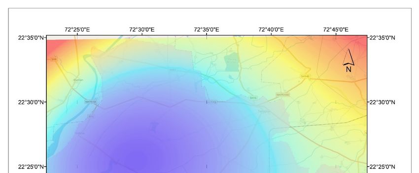
Water 2019, 11, 724                                                                                             5 of 15

analyzed by DIONEX ICS-90 ion chromatograph with an error percentage of less than 2%, using
duplicates. The major cations were evaluated by inductively coupled plasma-mass spectrometry
(ICP-MS) with a precision of less than 2%, using duplicates. For each instrument, after the analysis
of every five samples, one replicate was used to check the accuracy of the instruments. For major
ions, analytical precision was checked by normalized inorganic charge balance (NICB) [28]. This is
defined as [(Tz+ − Tz− )/(Tz+ + Tz− )] and represents the fractional difference between total cations
and anions. Here, Tz+ and Tz− represent the total mille-equivalent of cations and anions, respectively.
The observed charge balance supports the quality of the data points, which is better than ±5%, and
generally this charge imbalance was in favor of positive charge. For statistical analysis, a multivariate
analysis technique was used, where the data was subjected to correlation analysis using Spearman’s
rank coefficient ranking of the data and not their absolute value using Social Science Statistical Software
(SPSS) version 21.0.

3.2. Decadal Land Use Changes
     To quantify the decadal (2001–2011) land use changes, remotely sensed, multi-temporal satellite
data from the Landsat series (Thematic Mapper (TM) / Enhanced Thematic Mapper Plus (ETM+))
were used as the primary input. These satellite images, acquired on 10 November 2001 and 14
November 2011, respectively, were downloaded from the United States Geological Survey (https:
//earthexplorer.usgs.gov/). Both the images were subjected to a series of pre-processing techniques,
including geometric and radiometric correction, using the ErDAS ImagineTM 9.3 image processing
software. Both the images were spatially referenced in the Universal Transverse Mercator (UTM)
projection system (zone 43 north) with World Geodetic System (WGS) 1984 as datum. The details of
the satellite images, along with the bands used for this study are furnished Table 1.

                      Table 1. Details of the satellite data used for land use map preparation.

                                                               Spatial Resolution     Band Considered with
      Satellite/Sensor      Date of Pass        Path/Row
                                                                       (m)           Spectral Resolution (µm)
                                                                       30                 0.45–0.52 (blue)
          Landsat-7        10th November,                              30                0.52–0.60 (green)
                                                  148/45
            ETM+                2001                                   30                 0.63–0.69 (red)
                                                                       30                 0.77–0.90 (NIR)
                                                                       30                 0.45–0.52 (blue)
                           14th November,                              30                0.52–0.60 (green)
       Landsat-5 TM                               148/45
                                2011                                   30                 0.63–0.69 (red)
                                                                       30                 0.76–0.90 (NIR)

     For land use classification, both images were processed separately and were subjected to
supervised maximum likelihood classification using onscreen digitation of training polygons. Based
on the authors field experiences, a total of six major land use classes were present, including
(1) Agriculture, (2) Barren land, (3) Built-up areas, (4) Lake, (5) Marshland, and (6) River. Here,
barren land represents dryland ecosystem. The quality of the classified images was tested separately
for both the classified images through a rigorous accuracy assessment technique. We adopted the
confusion matrix approach to calculate the overall accuracy and kappa statistics. To compute this
matrix, 200 Ground Control Points (GCPs) were randomly generated and verified against the Google
EarthTM High-Resolution temporal images. The overall accuracy for the 2001 and 2011 land use were
observed 79.8 % and 81.2%, respectively.
     To identify the dominant changes in the land use category and to compute the spatial trend of
change, we utilized the change analysis tab onboard the Land Change Modeller of the TerrSetTM
geoprocessing software. At first, the land use maps from 2001 and 2011 were both calibrated using
the onboard harmonization tool to match the exact spatial extent and then, the status each pixel
from its initial (2001) to final (2011) state was compared. Thereafter, we cross-tabulated the loss and
gains among the six land use categories. To identify the patterns of changes, the spatial trend was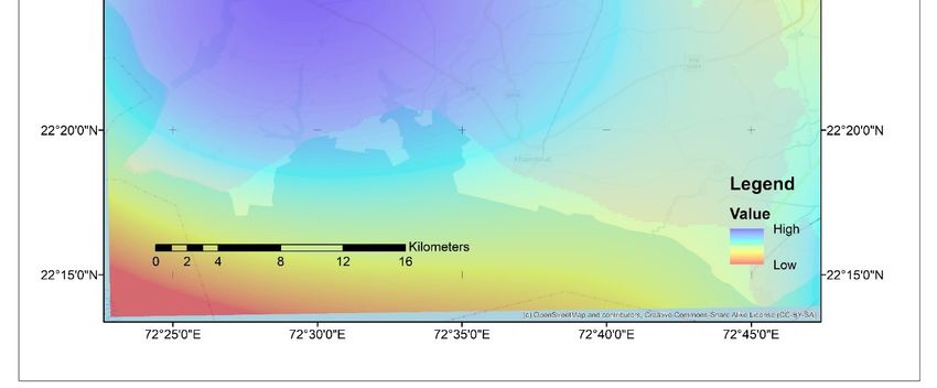
Water 2019, 11, x FOR PEER REVIEW 6 of 17
Water 2019, 11, 724 6 of 15
way to visualize and understand underlying drivers of change, and a third-order polynomial is
generally
mapped usingpreferred for thispolynomial
the third-order purpose [29].
to fit the changed pixel. Identification of spatial trends is an
effective way to visualize and understand underlying drivers of change, and a third-order polynomial
3.3. Preparation
is generally of Contour
preferred for thisMaps and [29].
purpose Spatial Analysis of the Impacts of LU Changes of GW Quality
To create the temporal contour maps of Cl− and NO3−, we applied the Inverse distance-weighted
3.3. Preparation of Contour Maps and Spatial Analysis of the Impacts of LU Changes of GW Quality
(IDW) interpolation technique to compute the contour profile from 64 sampling points. IDW is an
algorithm
To create widely used contour
the temporal to spatially
mapsinterpolate NO3 −data,
of Cl− andpoint and allows
, we applied for estimating
the Inverse the values at
distance-weighted
locations
(IDW) other than
interpolation the measured
technique sample
to compute thepoints.
contourIt profile
works from
on the64assumption that each
sampling points. IDW measured
is an
point has
algorithm a localused
widely influence that fades
to spatially with distance,
interpolate and the
point data, andhighest
allowsinfluences are always
for estimating close to
the values at the
point of observations. Thereafter, we classified the predicted groundwater quality
locations other than the measured sample points. It works on the assumption that each measured 3−), (Cl − and NO
well
point hasdepth and
a local water level
influence that contours,
fades withasdistance,
shown in andFigures 3a,b, 4influences
the highest and 5, respectively,
are alwaysand closeresampled
to the
theofcontour
point maps toThereafter,
observations. 30 m spatial weresolution to match
classified the that groundwater
predicted of the land use maps.(Cl
quality All− spatial
and NO −
analysis
3 ),
wellwas conducted
depth and waterin ArcGIS 10.5TM. as
level contours, Toshown
understand the influence
in Figure of the
3a,b, Figures six land
4 and use categories
5, respectively, and on
groundwater
resampled quality,
the contour mapsthe zonal
to 30 mstatistics
spatial tool in ArcGIS
resolution was applied.
to match This
that of the tooluse
land summarizes
maps. All the values
spatial
of a raster
analysis against the
was conducted in zones
ArcGIS of10.5TM.
anotherTo dataset, and results
understand are reported
the influence of the in
sixform
land ause
table. Here, we
categories
used the tool to
on groundwater compute
quality, thethe maximum,
zonal statisticsminimum and average
tool in ArcGIS values This
was applied. of Cl−tool
andsummarizes
NO3− for each theland
use of
values category,
a rasterin both 2001
against and 2011,
the zones respectively.
of another dataset, and results are reported in form a table. Here,
we used the tool to compute the maximum, minimum and average values of Cl− and NO3 − for each
land use category, in both 2001 and 2011, respectively.
Figure 3. Spatio-temporal distribution of Cl− (a,b) and NO3 − (c,d) in the study area.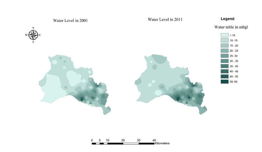
Figure 3. Spatio-temporal distribution of Cl (a, b) and NO3 (c, d) in the study area.

 Water 2019, 11, x FOR PEER REVIEW                                                                        7 of 17
Water 2019, 11, 724                                                                                            7 of 15
                Figure 3. Spatio-temporal distribution of Cl− (a, b) and NO3− (c, d) in the study area.

                         Figure 4. Spatial distribution of well depth in the study area.

                           Figure 4. Spatial distribution of well depth in the study area.

                           Figure 4. Spatial distribution of well depth in the study area.

           Figure 5. Spatio-temporal distribution of water level in year 2001 and 2011 in the study area.

4. Results

4.1. Water Quality Changes
     From the well depth of the sampling point (Figure 4), it is found that most of the shallow aquifers
are located in north and northwestern region, whereas medium to deep aquifers are located in the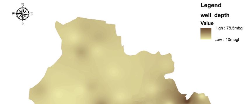
Water 2019, 11, 724                                                                                         8 of 15

south and southeast parts of the study area. Figure 5 shows the change in water level in the monitored
wells from 2001 to 2011. It is found that water level changed significantly, especially for the shallow
aquifers. A summary of the water quality of the groundwater samples for both 2001 and 2011 is
supplied in Table 2. The results suggest that the anionic abundance was in the order of Cl− > HCO3 −
> SO4 2− > NO3 − > PO4 3− , while cationic abundance was found in the order of Mg2+ > Ca2+ > Na+
> K+ . Here, most of the parameters are within the permissible limits prescribed by [13,14], with the
exceptions of Cl− in both 2011 and 2011 and NO3 − in 2011. Also, it is found that the water level in
2011 was lower, with an average of 3.9 m dropdown, which was primarily due to the high usage rate
(Table 2). To evaluate the effects of well depth, we plotted the relationship between NO3 − and Cl−
and well sampling depth, as shown in Figure 6a,b, respectively. Also, from the spatial distribution of
changes in NO3 − and Cl− concentrations shown in Figure 3, it was found that shallow aquifers were
mainly affected by nitrate enrichment in the year 2011 (Figure 6a), which at spatial scale corresponded
to the sample numbers ranging from 40–64 (Figure 1), which were collected from regions dominated
by agricultural activities (as seen in Figure 3c,d). Most of the sampling location also lies in the northern
and northwestern part, near to the river, as shown in Figure 1, where because of high water table
and fertile land, agricultural activities have intensified over the last decade and resulted in nitrate
enrichment. Looking into the temporal variation of Cl− concentration with depth, a temporal shift
in sea water–fresh water interface is observed, as shown in the shaded rectangle (6b), which results
in a higher concentration of chloride in deeper wells, too. This is a clear case of salt-water intrusion
because of the higher groundwater extraction. For chloride, the maximum deviation was found in
sample numbers ranging from 31–37, which lay mainly in the southern part or coastal region of the
study area, as shown in Figure 1, which signifies the impact of the coastal environment and/or local
anthropogenic activities in the region.

                      Table 2. Statistical summary of water quality for the years 2001 and 2011.

                                                 2001                                  2011
              Parameter             Range       Average      St Dev       Range        Average     St Dev
          Well depth (mbgl)        10.0–90.0       30.8        18.0       10.0–90.0      30.8        18.0
          Water level (mbgl)       4.0–73.5        18.2        13.9       6.0–78.0       22.1       15.0
                  pH                6.8–7.8         7.3         0.3        6.4–7.7        7.4        0.5
             EC (µs/cm)          362.0–8230.0     572.3       271.0     478.0–9792.0    837.8       415.0
             Na+ (mg/L)           29.0–611.7       81.6       112.2      41.1–737.5      99.4      135.9
             K+ (mg/L)             4.2–36.7        14.4         8.9       4.2–36.7       19.7        8.9
            Ca2+ (mg/L)           13.8–251.6      101.2        10.1      40.2–303.7     138.0       34.7
            Mg2+ (mg/L)            6.0–424.7      186.1        36.6      11.5–558.6     215.9       107.7
           HCO3 − (mg/L)         62.1–1032.3      156.5       135.6     68.2–1204.8     180.3      201.5
           SO4 2− (mg/L)          13.3–234.8       42.4        25.7      20.0–366.7      63.3       76.1
             Cl− (mg/L)           9.8–4874.9      375.1       862.6     31.0–5804.5     570.8      1004.3
           NO3 − (mg/L)            8.9–119.8       38.6        23.9      12.1–211.9      73.1        45.4
           PO4 3− (mg/L)           1.3–44.1         3.9         5.6       5.4–78.6        5.7       20.2

4.2. Land Use Changes
     Land use maps for both year 2001 and 2011, derived from the Landsat satellite images, are shown
in Figure 7. A statistical summary of the spatial extent of each land use class in each year is presented
in Table 3. For the year 2001, the most dominant feature was barren land, having an area of 465.64 km2
(54.45% of the study area), and lying mainly in the southeast region of the study area. Barren land
was followed by agriculture, which made up approximately 35.44% of total area and was spread
mainly around the river and in the north and northwestern region of the study area. This was followed
by marshland, which occupied around 4% of the study area. Marshland includes both fresh water
marshes because of the presence of river and lake, and salty marshes due to presence of estuary in
the southern part of this study area. Marshland was followed by built-up area, with 3.7% of the total
area sparsely distributed in both the north and south regions. The fifth category is river, which is the
presence of the Mahi River flowing from the north to the south direction. The last class is lake, which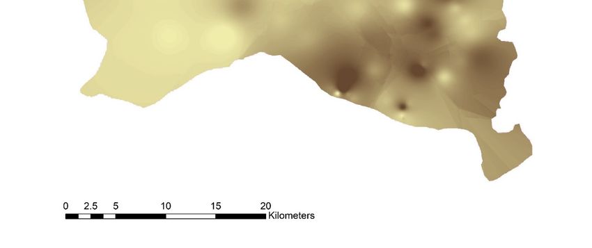
Water 2019, 11, 724                                                                                                                                              9 of 15

occupies about 1.8% of the total area and is located in the northern part of the study area. Looking at
the map for the year 2011, significant changes were observed for almost all of the land-use categories
except for lake and river. The most drastic changes were observed for agricultural and barren land
categories. It was found that nearly all of the barren land that was lost was due to conversion to
agricultural lands. This change can be attributed to a recent increase in agricultural activity to meet
the food demand of the newly developed human settlements. Changes in the marshlands and lakes
were mainly attributed to coastal development, and human encroachment of water bodies for urban
sprawl. To support the finding, cubic trend considered the conversion of barren land to agricultural
land, which seems to be the most dominant driver of decadal land change (Figure 8). Here, it is evident
that the conversion was highest in the central and southwest parts of the study area, in proximity to
the river. The most obvious reason behind this trend is the presence of riparian fertile land and shallow
aquifers,  as mentioned
    Water 2019,             above.
                11, x FOR PEER REVIEW                                                                   9 of 17

                        350                                                                                                   90
                                           NO3- (2001)
                                           NO3- (2011)                                                              (a)       80
                        300                Water level (2001)
                                           Water level (2011)                                                                 70

                                                                                                                                       Water level (mbgl)
                        250
                                                                                                                              60
         NO3- (mg/L)

                        200                                                                                                   50

                        150                                                                                                   40

                                                                                                                              30
                        100
                                                                                                                              20

                        50
                                                                                                                              10

                         0                                                                                                    0
                              1 3 5 7 9 11 13 15 17 19 21 23 25 27 29 31 33 35 37 39 41 43 45 47 49 51 53 55 57 59 61 63 65

                  10000                                                                                                           90
                                    Saltwater                                                       Cl- (2001)      (b)
                                    intrusion                                                       Cl- (2011)                    80
                                                                                                                                                  Water level (mbgl)

                                                                                                    Water level (2001)
                                                                                                                                  70
                       1000                                                                         Water level (2011)
                                                                                                                                  60
     Cl- (mg/L)

                                                                                                                                  50
                        100
                                                                                                                                  40

                                                                                                                                  30
                         10
                                                                                                                                  20

                                                                                                                                  10

                          1                                                                                                       0
                              1 3 5 7 9 11 13 15 17 19 21 23 25 27 29 31 33 35 37 39 41 43 45 47 49 51 53 55 57 59 61 63 65

                                                                 Sample number

       Figure 6. Spatial distribution of (a) NO3 − and (b) Cl− in the groundwater with relation to water level.
           Figure 6. Spatial distribution of (a) NO3− and (b) Cl− in the groundwater with relation to water level.

    4.1. Land Use Changes
         Land use maps for both year 2001 and 2011, derived from the Landsat satellite images, are shown
    in Figure 7. A statistical summary of the spatial extent of each land use class in each year is presented
    in Table 3. For the year 2001, the most dominant feature was barren land, having an area of 465.64
    km2 (54.45% of the study area), and lying mainly in the southeast region of the study area. Barren
marshlands and lakes were mainly attributed to coastal development, and human encroachment of
water bodies for urban sprawl. To support the finding, cubic trend considered the conversion of
barren land to agricultural land, which seems to be the most dominant driver of decadal land change
(Figure 8). Here, it is evident that the conversion was highest in the central and southwest parts of
the study area, in proximity to the river. The most obvious reason behind this trend is the presence
Water 2019, 11, 724 10 of 15
of riparian fertile land and shallow aquifers, as mentioned above.
Water 2019, 11, x FOR PEER REVIEW 11 of 17
Figure 7. Land use/land cover map of the study area for the year 2001 and 2011.
Figure 7. Land use/land cover map of the study area for the year 2001 and 2011.
Figure8.8.Spatial
Figure Spatialtrend
trend showing
showing the conversionof
the conversion ofbarren
barrenland
landtotoagricultural
agriculturalland.
land.
Table 3. Statistical summary for various categories in land use/land cover maps for the years 2001
and 2011.
2001 2011
LULC Area Proportion Area Proportion Change in the Change in Proportion
(Category) (km2) (%) (km2) (%) Area (%)Water 2019, 11, 724 11 of 15
Table 3. Statistical summary for various categories in land use/land cover maps for the years 2001
and 2011.
2001 2011
LULC Area Proportion Area Proportion Change in Change in
(Category) (km2 ) (%) (km2 ) (%) the Area Proportion (%)
Agriculture 303.06 35.44 344.81 40.32 41.75 4.88
Barren land 465.64 54.45 429.45 50.21 −36.19 −4.23
Built-up 31.67 3.70 42.32 4.95 10.65 1.25
Lake 6.83 0.80 6.33 0.74 −0.50 −0.06
Marshland 33.87 3.96 18.96 2.22 −14.91 −1.74
River 14.18 1.66 13.37 1.56 −0.81 −0.09
4.3. Relationship between Land Use Change and Water Quality
To evaluate the impact of land use on groundwater quality, the principal changes among the
different categories between the years 2001 and 2011 are shown in Figure 9. As can be seen in this map,
five major types of land-use transitions took place between the two years, namely the conversions
from: barren land to agricultural land, agricultural land to barren land, built-up land to barren
land, marshland to barren land, and barren land to built-up land. Among the above-mentioned five
categories, conversion from barren land to agriculture was most dominant, and should be one of the
main drivers of groundwater change. The barren land to agricultural land change was most prevalent
Water 2019, 11, x FOR PEER REVIEW 12 of 17
in the western half of the study area. Geologically, this area is alluvial fertile land with a high water
table. This triggered
well supported a swift
by both increase
Figure in agricultural
3, i.e., practices,ofwhich
spatial distribution is well
nitrate, and supported
Figure 6a, by
i.e.,both Figurein3,
changes
i.e., spatial distribution
nitrate with well depth. of nitrate, and Figure 6a, i.e., changes in nitrate with well depth.
Figure
Figure 9. Principal
9. Principal changes
changes among
among different
different categories
categories in land
in land use/land
use/land cover
cover from
from year
year 2001
2001 to to
2011.
2011.
4.4. Zonal Statistics
Finally, zonal statistics was calculated to estimate the association between different land
categories and changes in mean concentration for both NO3− and Cl−, as shown in Figure 10a,b,
respectively. The order of influence of each land use type on NO3− concentrations in the groundwaterWater 2019, 11, 724 12 of 15
4.4. Zonal Statistics
Finally, zonal statistics was calculated to estimate the association between different land categories
and changes in mean concentration for both NO3 − and Cl− , as shown in Figure 10a,b, respectively.
The order of influence of each land use type on NO3 − concentrations in the groundwater was
agricultural land > bare land > lake > marshland > built-up > river, with the magnitude of NO3 −
Water 2019, 11, x FOR PEER REVIEW 13 of 17
concentrations from 2001 to 2011 increasing by factors of 11.9, 9.7, 7.4, 6.3, 4.9 and 3.6, respectively.
600
NO3- (mean_2001) (mg/L) NO3- (mean_2011) (mg/L)
500
NO3- (mg/L)
(a)
400
300
200
100
0
Agriculture Bareland Builtup Lake Marshland River
700
Cl- (mean_2001) (mg/L) Cl- (mean_2011) (mg/L)
600
500 (b)
Cl- (mg/L)
400
300
200
100
0
Agriculture Bareland Builtup Lake Marshland River
Land use categories
Zonal statistics − and
Figure 10.10.
Figure Zonal statisticsfor
fordifferent
differentland
landuse
usecategories
categories responsible
responsible for changes
changesin
inthe
the(a)
(a)NO
NO3−3and
Cl−
(b)(b) Clin groundwater.
− in groundwater.
Agricultural
Agriculturalpractices
practices inin the
the farmlands
farmlands and converted
converted barren
barrenland
landinvolving
involvinghigh
highuseuseof of
fertilizers causes
fertilizers nitrate
causes enrichment
nitrate enrichment in the shallow
in the aquifers,
shallow especially,
aquifers, because
especially, of high
because leaching
of high ability.
leaching
The process
ability. of process
The nitrification responsibleresponsible
of nitrification for the conversion
for the of ammoniaofwithin
conversion nitrogen
ammonia fertilizers
within nitrogeninto
fertilizers
nitrate into nitrate
is shown is shown(1):
with Equation with Equation (1):
NH + 2O → NO + H + H O (1)
Next, bare land has a high increase in NO3− concentration compared to the other classes. This is
because bare land is typically located near to agricultural land, so it is affected by the nearby fertilizer
use. The next most dominant land use category is lake, as lakes act as a receiving body for locally
generated nitrate-enriched runoff, which is quite evident with algal blooms in the lake throughout
the year. This nitrate-enriched lake water recharges shallow aquifers, and thus contributes toWater 2019, 11, 724 13 of 15
NH3 + 2O2 → NO3− + H+ + H2 O (1)
Next, bare land has a high increase in NO3 − concentration compared to the other classes. This is
because bare land is typically located near to agricultural land, so it is affected by the nearby fertilizer
use. The next most dominant land use category is lake, as lakes act as a receiving body for locally
generated nitrate-enriched runoff, which is quite evident with algal blooms in the lake throughout the
year. This nitrate-enriched lake water recharges shallow aquifers, and thus contributes to increasing
the concentration of nitrate in the nearby groundwater sources. Following this, the next land use
category in terms of contribution to nitrate enrichment is marshland. Because of the very little amount
of water in the marshlands in this area, particularly during the dry season, decomposing organic
matter leads to nitrate enrichment, which finally seeps into groundwater sources nearby. Marshland
was followed by built-up in terms of the land uses responsible for high nitrate concentration in the
groundwater. High nitrate in the groundwater here can be attributed to leaching from open dump
yard sites, landfills, untreated domestic sewerage and industrial effluents. Finally, river is the least
contributing land use type for nitrate enrichment in the groundwater samples, probably because they
transport the nitrate runoff that they receive to the nearby sea.
In terms of concentrations of Cl− in the groundwater, the order of influence for the different land
use categories was marshland > built-up > agriculture > bare land > lake > river, with the magnitude
of Cl− concentrations increasing between 2001–2011 by factors of 1.75, 1.73, 1.63, 1.51, 1.41 and 1.26 in
each land use category, respectively. The largest contribution here is from marshland located near the
coastal region in the southern end of the study area. This is mainly a mixture of salt marshes and tidal
marshes. Because of the high contribution from sea tides, the Cl− concentration in the groundwater
increases. This was followed by built-up, agriculture and barren land. This can all sum up the pressure
from anthropogenic activities on groundwater development mainly in the southern part of the study
area. Because of the increase in demand for groundwater for agriculture and household consumption,
the seawater–groundwater equilibrium has become disturbed, and brackish plumes are encroaching
into the inland shallow aquifers, as evident from the elevated Cl− concentrations in the groundwater.
Other possible reasons for the higher groundwater salinity may include high evaporation rate during
recharge and increased infiltration of sewage effluents. Lastly, lakes and rivers had the least impact on
the elevated Cl− concentrations found in the groundwater.
To support the above finding, correlation analysis was performed, and the results are shown
in Table 4. It gave a clear picture to trace the prime factors responsible for the change in water
quality parameter (NO3 − and Cl− ) concentrations. It was found that changes in land use categories
like agriculture and built-up and water level have a significant positive correlation with change in
NO3 − concentrations, whereas they were negatively correlated with barren land. This supports
the arguments that with an increase in population growth, agricultural practices and built-up areas
increases at the cost of other land cover type namely barren land, marshland, etc. Thus, high usage
of fertilizers in agricultural activities and leakage from untreated sewerage in the rapidly urbanizing
areas leads to increase in NO3 − concentrations in the groundwater. Also, these combined activities
caused a disturbance in sea water-fresh water equilibrium in the coastal part of the study areas.
As a result, the effect of groundwater salinization increased, and hence so did the Cl− concentration in
the groundwater.
The above-mentioned poor management of water resources has resulted in environmental
deterioration, increases in water-related health diseases, and loss of income for farmers, among other
problems in the last few years. Henceforth, as a mitigation measure for the above issues related to
water scarcity, there is a need for better policy implementation regarding water resource management,
including management of data inventory for both water quality and budget, conjunctive use of both
surface and groundwater, and citizen awareness; all of these aspects are matters for future research.Water 2019, 11, 724 14 of 15
Table 4. Correlation matrix showing relationship change in LULC and water quality parameters from
2001 to 2011.
Barren Marsh Water Level
Agriculture Built-Up Lake River Nitrate Chloride
Land Land Reduction
Agriculture 1.00
Barren land −0.78 1.00
Built-up 0.59 −0.62 1.00
Lake 0.12 0.16 0.40 1.00
Marsh land −0.51 0.20 0.37 0.03 1.00
River −0.22 −0.13 0.06 0.09 0.08 1.00
Nitrate 0.84 −0.65 0.55 0.41 −0.44 0.45 1.00
Chloride 0.47 0.33 0.17 0.12 0.67 0.36 0.24 1.00
Water level reduction 0.79 −0.45 0.88 −0.23 −0.31 −0.28 0.66 0.80 1.00
5. Conclusions
The findings from this work revealed that the major factors for the change in the groundwater
quality between 2001–2011 in Khambhat city were the rising water demand along with groundwater
withdrawal (for domestic, agricultural and industrial need) and land use/land cover changes. As a
result of the above-mentioned drivers and pressures, sharp declines in fresh water resources in terms
of both quality (high nutrient content, salt water intrusion) and quantity (lowering of water table)
have been observed. More precisely, NO3 − concentration in the groundwater increased mainly for the
shallow wells near the agricultural field because of high fertilizers input, whereas Cl− concentration
in the groundwater increased for the samples located near the coast due to high water extraction
and salt-water intrusion. The vulnerability of these water resources can be further exacerbated by
different climate-related pressures like climate change, especially rainfall and temperature. This
study will be helpful for both scientific communities and decision makers involved in water resource
management. The poor management of water resources results in environmental deterioration,
increases in water-related health diseases, and loss of income for farmers, among other problems.
As a mitigation measure for the above issues related to water scarcity, there is a need for better policy
implementation regarding water resource management, including management of data inventory for
both water quality and budget, conjunctive use of both surface and groundwater, and citizen awareness.
Author Contributions: Conceptualization (P.K. and R.D.); methodology, (P.K. and R.D.); software, (P.K. and R.D.);
validation, (P.K. and R.D.); formal analysis, (P.K. and R.D.); investigation, (P.K. and R.D.); writing—original draft
preparation, (P.K. and R.D.); writing—review and editing, (P.K., R.D., B.A.J., C.S., M.B., M.K., B.K.M.).
Conflicts of Interest: The authors declare no conflict of interest.
References
1. Dabrowski, J.M.; De Klerk, L.P. An Assessment of the Impact of Different Land Use Activities on Water
Quality in the Upper Olifants River Catchment. Water Sa 2013, 39, 231–241. [CrossRef]
2. Saraswat, C.; Mishra, B.K.; Kumar, P. Integrated urban water management scenario modeling for sustainable
water governance in Kathmandu Valley, Nepal. Sustain. Sci. 2017, 12, 1037–1053. [CrossRef]
3. Chu, H.J.; Liu, C.; Wang, C. Identifying the Relationships Between Water Quality and Land Cover Changes in
the Tseng-Wen Reservoir Watershed of Taiwan. Int. J. Environ. Res. Public Health 2013, 10, 478–489. [CrossRef]
4. Gardner, K.K.; Vogel, R.M. Predicting Ground Water Nitrate Concentration from Land Use. Ground Water
2005, 43, 343–352. [CrossRef] [PubMed]
5. Zeilhofer, P.; Lima, E.B.N.R.; Lima, G.A.R. Spatial patterns of water quality in the Cuiaba river basin, Central
Brazil. Environ. Monit. Assess. 2006, 123, 41–62. [CrossRef] [PubMed]
6. Ding, J.; Jiang, J.; Fu, L.; Liu, Q.; Peng, Q.; Kang, M. Impacts of Land Use on Surface Water Quality in a
Subtropical River Basin: A Case Study of the Dongjiang River Basin, Southeastern China. J. Water 2015, 7,
4427–4445. [CrossRef]
7. United Nation Sustainable Development Goals. The 2030 Agenda for Sustainable Development; A/RES/70/1;
United Nation Sustainable Development Goals: New York, NY, USA, 2015; p. 41.Water 2019, 11, 724 15 of 15
8. Keesstra, S.; Mol, G.; de Leeuw, J.; Okx, J.; de Cleen, M.; Visser, S. Soil-related sustainable development goals:
Four concepts to make land degradation neutrality and restoration work. Land 2018, 7, 133. [CrossRef]
9. Steyl, G.; Dennis, I. Review of coastal-area aquifers in Africa. Hydrogeol. J. 2010, 18, 217–225. [CrossRef]
10. Anderson, F.; Al-Thani, N. Effect of Sea Level Rise and Groundwater Withdrawal on Seawater Intrusion in
the Gulf Coast Aquifer: Implications for Agriculture. J. Geosci. Environ. Prot. 2016, 4, 116–124. [CrossRef]
11. Grundmann, J.; Khatri, A.A.; Schütze, N. Managing saltwater intrusion in coastal arid regions and its societal
implications for agriculture. Proc. IAHS 2016, 373, 31–35. [CrossRef]
12. Puckett, L. Nonpoint and Point Sources of Nitrogen in Major Watersheds of the United States; USGS Water
Resources Investigations Report 94–4001; United States Geological Survey: Reston, VA, USA, 1994.
13. Pérez-Fernández, M.A.; Calvo-Magro, E.; Valentine, A. Benefits of the symbiotic association of shrubby
legumes for the rehabilitation of degraded soils under Mediterranean climatic conditions. Land Degrad. Dev.
2016, 27, 395–405. [CrossRef]
14. WHO. Guidelines or Drinking-Water Quality, 4th ed.; World Health Organization: Geneva, Switzerland, 2011; p. 563.
15. Bureau of Indian Standards (BIS). Indian Standard Drinking Water Specification, 2nd ed.; BIS 10500:2012; Bureau
of Indian Standards: New Delhi, India, 2012.
16. Manassaram, D.M.; Backer, L.C.; Messing, R.; Fleming, L.E.; Luke, B.; Monteilh, C.P. Nitrates in drinking
water and methemoglobin levels in pregnancy: A longitudinal study. Environ. Health 2010, 9, 60. [CrossRef]
17. Alfarrah, N.; Walraevens, K. Groundwater overexploitation and seawater intrusion in coastal areas of arid
and semi-arid regions. Water 2018, 10, 143. [CrossRef]
18. Kumar, P. Multi isotopic approach to study temporal variation of groundwater quality in coastal aquifer of
Saijo Plain, Shikoku Island, Japan. Water Resour. 2013, 40, 208–216. [CrossRef]
19. Hua, A.K. Land use land cover changes in detection of water quality: A study based on remote sensing and
multivariate statistics. J. Environ. Public Health 2017, 2017, 7515130. [CrossRef]
20. Huang, J.; Zhan, J.; Yan, H.; Wu, F.; Deng, X. Evaluation of the impacts of land use on water quality: A case
study in the Chaohu Lake Basin. Sci. J. 2013, 2013, 329187. [CrossRef]
21. Khan, A.; Khan, H.H.; Umar, R. Impact of land-use on groundwater quality: GIS-based study from an
alluvial aquifer in the Western Ganges Basin. Appl. Water Sci. 2017, 7, 4593–4603. [CrossRef]
22. Narany, T.S.; Aris, A.Z.; Sefie, A.; Keesstra, S. Detecting and predicting the impact of land use changes on
groundwater quality, a case study in Northern Kelantan, Malaysia. Sci. Total Environ. 2017, 599–600, 844–853.
[CrossRef]
23. Persky, J.H. The Relation of Ground-Water Quality to Housing Density; USGS Water Resources Investigation
Report 86-4093; USGS: Cape Cod, MA, USA, 1986.
24. Kumar, P.; Kumar, A.; Singh, C.K.; Saraswat, C.; Avtar, R.; Ramanathan, A.L.; Herath, S. Hydrogeochemical
Evolution and Appraisal of Groundwater Quality in Panna District, Central India. Expo. Health 2016, 8,
19–30. [CrossRef]
25. Sarangi, R.K.; Chauhan, P.; Nayak, S.R. Inter-annual variability of phytoplankton blooms in the northern
Arabian Sea during winter monsoon period (February-March) using IRS-P4 OCM data. Indian J. Mar. Sci.
2005, 34, 163–173.
26. Kumar, N.; Kumar, P.; Basil, G.; Kumar, R.; Kharrazi, A.; Avtar, R. Chemo-metric analysis for evaluating
geochemical processes responsible for spatio-temporal variation of surface water quality at Narmada
estuarine region in Gujarat, India. Appl. Water Sci. 2015, 5, 261–270. [CrossRef]
27. Central Ground Water Board (CGWB). District Groundwater Brochure; CGWB: Anand District, Gujarat, India,
2013; p. 20.
28. Kumar, P.; Kumar, M.; Ramanathan, A.L.; Tsujimura, M. Tracing the factors responsible for arsenic enrichment in
groundwater of the middle Gangetic Plain, India: A sourec identification perspective. Environ. Geochem. Health
2010, 32, 129–146. [CrossRef] [PubMed]
29. Yen, S.T.; Liu, S.; Kolpin, D.W. Analysis of nitrate in near-surface aquifers in the Midcontinental United
States: An application of the inverse hyperbolic sine Tobit model. Water Resour. Res. 1996, 32, 3003–3011.
[CrossRef]
© 2019 by the authors. Licensee MDPI, Basel, Switzerland. This article is an open access
article distributed under the terms and conditions of the Creative Commons Attribution
(CC BY) license (http://creativecommons.org/licenses/by/4.0/).You can also read