Circulation Specific Precipitation Patterns over Svalbard and Projected Future Changes - MDPI
←
→
Page content transcription
If your browser does not render page correctly, please read the page content below
atmosphere
Article
Circulation Specific Precipitation Patterns over
Svalbard and Projected Future Changes
Andreas Dobler *, Julia Lutz, Oskar Landgren           and Jan Erik Haugen
 Norwegian Meteorological Institute, Henrik Mohns plass 1, 0313 Oslo, Norway; julial@met.no (J.L.);
 oskaral@met.no (O.L.); janeh@met.no (J.E.H.)
 * Correspondence: andreas.dobler@met.no

 Received: 27 November 2020; Accepted: 14 December 2020; Published: 21 December 2020

 Abstract: Precipitation on Svalbard can generally be linked to the atmospheric circulation in the
 Northern Atlantic. Using an automated circulation type classification, we show that weather type
 statistics are well represented in the Max Planck Institute Earth System Model at base resolution
 (MPI-ESM-LR). For a future climate projection following the Representative Concentration Pathway
 scenario RCP8.5, we find only small changes in the statistics. However, convection permitting
 simulations with the regional climate model from the Consortium for Small-scale Modeling in climate
 mode (COSMO-CLM) covering Svalbard at 2.5 km demonstrate an increase in precipitation for all
 seasons. About 74% of the increase are coming from changes under cyclonic weather situations.
 The precipitation changes are strongly related to differences in atmospheric conditions, while the
 contribution from the frequencies of weather types is small. Observations on Svalbard suggest that the
 general weather situation favouring heavy precipitation events is a strong south-southwesterly flow
 with advection of water vapour from warmer areas. This is reproduced by the COSMO-CLM
 simulations. In the future projections, the maximum daily precipitation amounts are further
 increasing. At the same time, weather types with less moisture advection towards Svalbard are
 becoming more important.

 Keywords: convection permitting climate modelling; COSMO-CLM; Svalbard; precipitation; integrated
 water vapour; projections; RCP8.5; atmospheric circulation patterns; weather type classification

1. Introduction
     During recent decades, an increase in the frequency and intensity of heavy precipitation events
on Svalbard has been reported [1]. These events frequently result in landslides, avalanches and
flooding [2,3]. Even in midwinter, with a mean temperature well below −10 °C at the western coast of
Svalbard, large precipitation amounts can fall as rain on warmer days [4], often driven by the advection
of high amounts of water vapour from southern moisture sources over the Atlantic. The moisture is
transported towards the northern end of the North Atlantic cyclonic track where the archipelago is
located, and are linked to “atmospheric river”-like features in the precipitable water anomaly field [5].
     For Svalbard, an increase in mean precipitation [6] as well as in daily precipitation extremes [1,7]
is projected towards the end of the century. Consistently, studies on future climate projections for
the Arctic [8,9] have demonstrated a much faster increase in precipitation than in the global mean.
While [9] attributes this mainly to an increased moisture transport from lower latitudes, ref. [10]
states that the increase is primarily due to an intensification of the local surface evaporation and more
precipitation can also be expected without changes in moisture advection. With our work we aim to
analyse the connection between large-scale atmospheric conditions and local-scale precipitation on
Svalbard. Several studies (e.g., [11–13]) have shown how changes in large-scale atmospheric conditions
have already contributed to a warmer climate in the North Atlantic region of the Arctic. To extend this

Atmosphere 2021, 11, 1378; doi:10.3390/atmos11121378                        www.mdpi.com/journal/atmosphere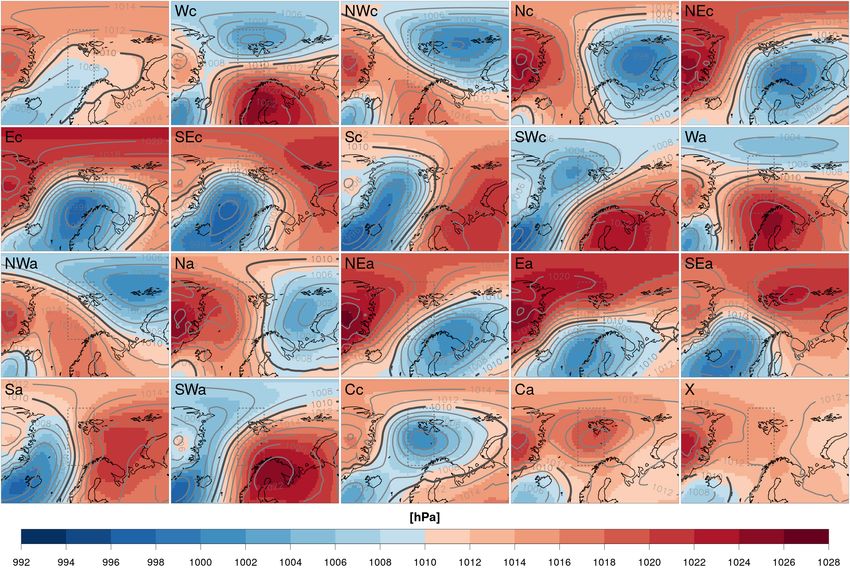
Atmosphere 2021, 11, 1378                                                                          2 of 20

to precipitation and future projections, our analysis includes the present and a possible future climate
following the Representative Concentration Pathway scenario RCP8.5 [14].
      Quality controlled meteorological station data from Svalbard are available for several decades,
the majority reconstructed back to 1948 [15]. Hence, there is a broad assessment of changes and trends
(e.g., [15–17]). However, as the stations are mostly located at the western coast, the climate and its
changes in other parts of the archipelago are still not well known [1]. Recent studies have though
attempted to fill this knowledge gap using satellite and reanalysis data [1,18].
      The results from studies on observational data provide the foundation for our understanding of
the physical processes involved. The intention of our current study is to confirm these findings in a
modelling framework, and extend the analysis to the whole of Svalbard and to possible future climate
conditions. In particular, the aim of our study is to answer the following questions:

•     How well are typical weather types around Svalbard represented in the modelling framework for
      the current climate?
•     What is the contribution from the different weather types to precipitation and its spatial
      distribution on Svalbard?
•     What may the atmospheric conditions and the frequencies of specific weather types look like in a
      future climate?
•     Which part of projected precipitation changes can be attributed to changes in frequencies of
      weather types and which part to changes in large-scale conditions?

     To answer these questions, our analysis includes local precipitation data from a regional climate
model (RCM). However, the existing RCM data basis for Svalbard is limited compared to other
European and Norwegian regions, both in terms of model resolution (50 km versus 12 km) and number
of simulations. Furthermore, there is a strong influence of local topography on heavy rainfall events
documented for Svalbard (e.g., [5]). Thus, the ability of an RCM to simulate these events depends
on an accurate representation of the orography [19], which is not the case at 50 km. As shown in
a study by [20] for a strong precipitation event over steep terrain in southern Norway, running an
RCM at a kilometer scale yields much better results than running it at larger scales when compared
to observational data. High-resolution RCM modelling is further supported by [21], showing that
resolving convection in RCMs (i.e., using a grid resolution of about 4 km or less) can provide a clear
added-value for model precipitation. This spatial resolution constraint limits our analysis to the use of
precipitation data from simulations at kilometer scale.
     This article is structured as follows. Section 2 describes the data and methods used for the weather
type classification and the associated precipitation patterns. The results of the analysis are presented
in Section 3 and discussed in Section 4. Finally, Section 5 provides brief conclusions of our findings.

2. Data and Methods

2.1. High-Resolution Climate Model and Simulations
     To provide high-resolution precipitation fields for Svalbard, convection permitting climate
simulations at 0.022° (approx. 2.5 km) have been carried out using the COSMO (Consortium
for Small-scale Modeling) model in climate mode (COSMO-CLM, see [22]). COSMO-CLM is a
non-hydrostatic model based on the COSMO numerical weather prediction model (www.cosmo-
model.org). It is the community model of the German regional climate research. More details on the
COSMO-CLM model can be found on www.clm-community.eu.
     The Svalbard simulation configuration for COSMO-CLM follows the setup used for simulations
carried out within the EURO-CORDEX initiative [23,24]. This includes a Kessler-type [25] microphysics
scheme with ice-phase processes for cloud water, rain and snow, and a radiation scheme following [26].
In the high-resolution simulation, no convection parametrisation is applied, avoiding one of the main
reasons for biases and uncertainties in climate models [21]. The model setup consists of 40 atmospheric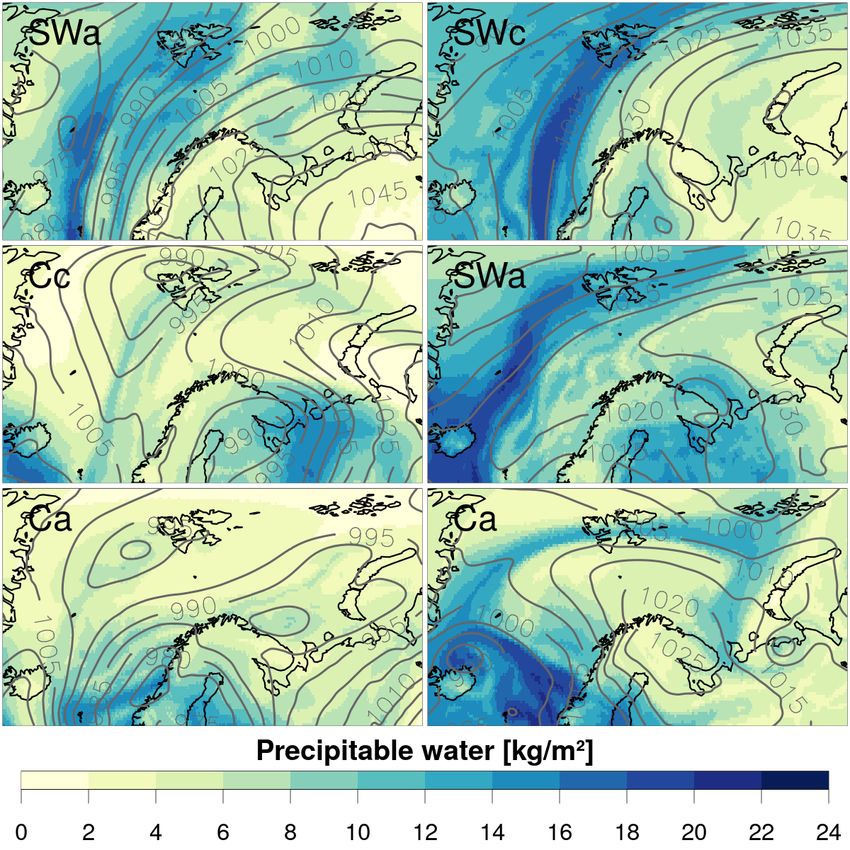
Atmosphere 2021, 11, 1378                                                                             3 of 20

layers reaching up to 23 km (approx. 40 hPa) and 9 soil layers down to 11.5 m. To account for spin-up,
the model has been initialised half a year before the actual simulation periods.
     ERA-Interim reanalysis [27] has been used as the driving model for a simulation covering
the time period 2004–2017. For the current and future climate projections following the RCP8.5
scenario, the global coupled Max Planck Institute Earth System Model at base resolution
(MPI-ESM-LR) model [28] has been downscaled covering the time periods 1971–2000 and 2071–2100.
The spatial resolution of the ERA-Interim and MPI-ESM-LR data is 0.7° and 1.875°, respectively.
Thus, an intermediate resolution model step at 0.22° has been used in both cases, to prevent a too large
resolution jump from the global forcing data to the high-resolution COSMO-CLM simulation at 0.022°.
The model orographies and domains for both model steps are shown in Figure 1.

      Figure 1. Orography in the intermediate (left) and high-resolution (right) regional climate model
      domain. The location of Svalbard Airport is indicated by a circle in the high-resolution domain.

      The intermediate resolution domain has a size of 248 × 123 grid points. It was selected to cover
the main moisture intrusion area for Svalbard, but also the Norwegian mainland, Svalbard itself and
the main parts of the “Norwegian Arctic”. Although the target area is located in the upper area of the
domain, there are at least 19 grid points in-between. The high resolution domain covers 354 × 264 grid
points with at least 44 grid points between the west coast and the boundary, and 35 grid points between
the north coast and the boundary, taking the recommendations in [29] into account. For both domains,
we did not see any inflow or outflow effects except some accumulation of precipitation in the outermost
10–12 boundary lines (not shown) which do not affect our results.
      An evaluation of the downscaling approach for Svalbard is given in [30], showing that the model
is able to reproduce the observed climate. Although COSMO-CLM shows too high precipitation values
in mountainous areas close to the coast and an underestimation of temperatures over land, the biases
are generally small. Furthermore, ref. [30] has shown that wind statistics for Svalbard Airport derived
from the COSMO-CLM model agree well with station data.

2.2. Classification of Atmospheric Circulation
     For the classification of atmospheric circulation we are following the objective method originally
proposed in [31] for the British Isles. As shown in [32], the method is able to reproduce the subjective
Lamb weather types [33] in an acceptable manner. A comprehensive description of the method is
given in [34]. The direction and strength of the mean flow and the vorticity are calculated based on
the variability of pressure in 16 selected grid points. This is followed by a set of rules that define the
weather types. The exact equations and the rules, as well as the adjustment needed for an application
in other areas than the British Isles, can be found in [34].
     Our classification setup distinguishes between 19 different Jenkinson-Collison Types (JCT),
consisting of 16 types denoting the dominant wind direction in 45° steps, together with the prevailing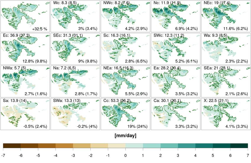
Atmosphere 2021, 11, 1378                                                                                  4 of 20

rotation (cyclonic or anticyclonic) and three types associated with pure cyclonic, pure anticyclonic or
light indeterminate flows, respectively. The classification area we use covers 3.75 to 21° E and 69 to
83.25° N. The area and the resulting grid points are shown in Figure 2. The centre of the area is located
south-west of Svalbard in order to have the main focus on the south-western parts of the main island
where most settlements are located. However, sensitivity tests for the location and size of the area
have shown a relative stable distribution of weather types. The specific area has been selected as it
reproduces the statistics from the atmospheric circulation calendar developed by [35] best.

      Figure 2. Annual and seasonal mean sea level pressure from ERA-Interim (1979–2008, as contour
      lines) and the current climate MPI-ESM-LR simulation (1971–2000, in colours). The numbered
      points and dashed box denote the grid points and bounding box used for the weather type
      classification, respectively. The labels in the top left corners refer to the annual mean (ANN) or the
      months of the specific season of the year.

     A FORTRAN routine to derive the JCT classification is available within a suite of more than
30 classification algorithms through the cost733class package [36]. The routine also includes an
adjustments according to the latitude of the classification area and the grid-point spacing.
     As input to the classification algorithm we used sea level pressure data at 12 UTC for each day.
For the reference classification, the data is coming from ERA-Interim reanalyses in the time period
1979–2008. For the climate simulations, the data is taken from the MPI-ESM-LR model in the time
periods 1971–2000 and 2071–2100, respectively. Additionally, integrated water vapour fields from the
MPI-ESM-LR driven intermediate resolution COSMO-CLM runs have been used to derive the amount
of precipitable water in the atmosphere for the analysis of a couple of heavy precipitation events.

2.3. Contribution from Frequencies and Large-Scale Conditions
     Based on the weather type classification, total precipitation differences can be decomposed
into two parts. The part resulting from differences in the frequencies of weather types can be
calculated using
                                                       n
                                                      ∑ ∆ fi · Pri
                                                                 re f
                                            ∆Pr f =                     ,                                      (1)
                                                      i =1
                                                                                re f
where ∆ f i is the difference in the frequency of weather type i, and Pri is the precipitation in the
reference data (i.e., the ERA-Interim or current climate MPI-ESM-LR simulation, respectively) for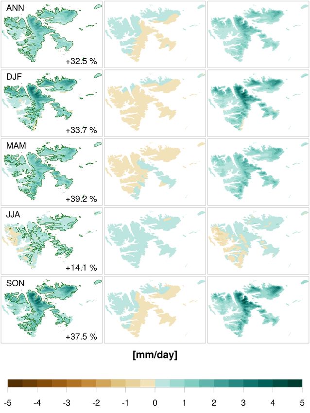
Atmosphere 2021, 11, 1378                                                                             5 of 20

weather type i. The second part, coming from the differences in large-scale conditions, can be
calculated by
                                                    n
                                                   ∑ fi
                                                          re f
                                          ∆Prc =                 · ∆Pri ,                                (2)
                                                   i =1
          re f
where f i is the reference frequency for weather type i, and ∆Pri is the precipitation difference for
weather type i.

2.4. Test for Statistical Significance
    All tests for statistical significant differences in this study have been carried out using a two-sample
Kolmogorov–Smirnov test [37] with a significance level α = 0.05.

3. Results

3.1. Simulation of the Current Climate
     To assess the performance of the MPI-ESM-LR model in the current climate, we analyse the
large-scale sea level pressure biases in the model and the monthly frequencies of the different weather
types. The COSMO-CLM precipitation fields associated with the different weather types are then
analysed with respect to the differences in the driving models, answering the question which parts can
be attributed to the differences in weather type frequencies and large-scale conditions, respectively.

3.1.1. Large-Scale Sea Level Pressure
      Figure 2 shows the annual and seasonal mean sea level pressure (SLP) from the ERA-Interim
reanalysis and MPI-ESM-LR model for the region -40 to 70 °E and 60 to 90 °N. According to [35],
the area shown provides “a good illustration of circulation patterns in the surroundings of Spitsbergen”.
Please note that in the regular latitude/longitude plots we are using, objects in the area close to the
top edge are actually smaller than they appear. However, we believe the projection is best suited to
illustrate geographical flow directions which are a key point of our analysis.
      As can be seen in Figure 2, the ERA-Interim data for winter (DJF) show a deep trough starting
at the Icelandic Low, covering the Norwegian Sea and reaching into the Barents Sea. Svalbard is
located at the northern edge of that trough, resulting in easterly air advection. For summer (JJA),
the SLP shows small horizontal gradients. Both during spring (MAM) and JJA, the SLP fields are
highly influenced by the Greenland High [35]. The autumn (SON) SLP pattern resembles the one from
winter but with a smaller pressure range. In the MPI-ESM-LR model, the mean patterns are similar
to ERA-Interim, and there are only small biases. Maps of the annual and seasonal mean biases are
shown in the supplementary materials. The largest biases occur in DJF, where the MPI-ESM-LR model
shows a high-pressure bias of about 4 hPa over the Kara sea west of Novaya Zemlya. This is a typical
problem in CMIP5 models [38] that is related to a too large ice cover in this area [30] and low-pressure
systems not penetrating far enough into the Barents Sea.

3.1.2. Weather Type Classification
     Monthly frequencies for the different weather types from ERA-Interim (Figure 3, left) show
that overall, a pure cyclonic situation (Cc) south-west of Svalbard is the most frequently detected
type. After that, northerly to south-easterly flows are dominating. In autumn, spring and winter,
the weather types NEc, Ec and SEc are most frequent (after Cc) and cyclonic types are more frequent
than anticyclonic ones. For summer, a pure anticyclonic situation (Ca) is most frequent. Summer also
shows the lowest cyclonic activity, especially for easterly advection (NEc to SEc), and the highest
frequencies of anticyclonic situations and the undefined weather type. In agreement with [39],
the winter season shows the most intense cyclonic activity.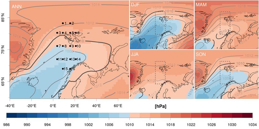
Atmosphere 2021, 11, 1378 6 of 20
Figure 3. Mean monthly occurrence of weather types in ERA-Interim (1979–2008, left) and the
MPI-ESM-LR current climate simulation (1971–2000, right), respectively. The dots mark statistically
significant differences.
In the MPI-ESM-LR simulation, the overall most frequent weather type is again a pure cyclonic
situation (Figure 3, right). Compared to ERA-Interim, the different weather types are more equally
distributed and there are overall more anticyclonic situations in the MPI-ESM-LR simulation. However,
there are only a few statistically significant differences, mostly apparent in summer.
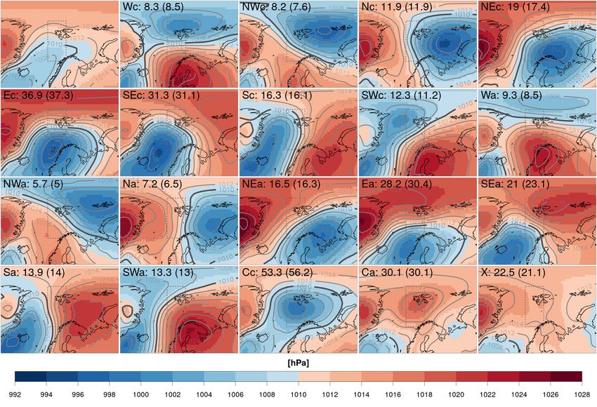
The typical mean sea level pressure patterns shown in Figure 4 are similar to the ones described
in [12], showing that our automated classification setup performs in a reasonable way. This is true
both for the MPI-ESM-LR and the ERA-Interim data. The differences in the patterns from the two
data sets are in the magnitude of 1–3 hPa. As already seen for the mean pressure fields (Figure 2),
the low pressure fields in MPI-ESM-LR are covering a smaller area than in ERA-Interim. Figure 4 also
demonstrates that the isobars in the MPI-ESM-LR model are generally more north-south oriented,
especially in SWa, SWc and Wc. For Sc, the low-pressure field between Greenland, Svalbard and
Norway is closer to the coast of Greenland in the MPI-ESM-LR model than in the ERA-Interim
reanalysis and does not extend as far to the north. Seasonal mean sea level pressure fields from
MPI-ESM-LR and ERA-Interim look similar to the annual patterns with the strongest gradients and
largest pressure ranges in winter and smoothed patterns in summer (not shown).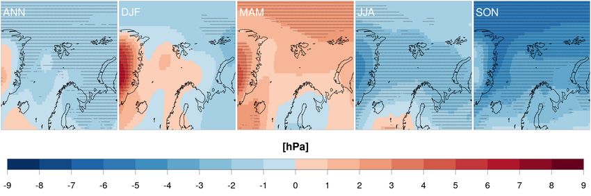
Atmosphere 2021, 11, 1378                                                                                   7 of 20

      Figure 4. Annual mean sea level pressure from MPI-ESM-LR (1971–2000, in colours) and ERA-Interim
      (1979–2008, as contour lines) for the current climate (top left) and the single weather types. The bold
      grey line shows the 1010 hPa level in the ERA-Interim fields and the dashed box the area used for the
      weather type classification. The labels in the top left corners refer to the weather type.

3.1.3. Local Precipitation
      Figure 5 shows the mean precipitation (over land) from the MPI-ESM-LR driven COSMO-CLM
for the current climate. The annual mean precipitation is 2.3 mm/day. The largest amounts are falling
at the south-eastern and western coast but the precipitation gradients are small in the annual mean.
For the different weather types, the precipitation patterns are clearly oriented towards the advection of
air with highest values on the windward side of the mountain ranges. The most contributing weather
types are Cc (26%), SEc (10%), Ec (9%) and Sc (8%). The lowest contributors are NWa (1.2%), Na (1.3%)
and NEa (2%). The Ea and SEa situations occur on about 20–30 days a year but precipitation is limited
to the south-eastern tip of Svalbard, thus their total contribution is also low. Also, a pure anticyclonic
situation (Ca) over Svalbard is detected at about 30 days per year, but the contribution to the total
precipitation is only 3.2%, indicating a generally dry weather situation. Under NEc conditions, some
precipitation is falling at the eastern coast, especially in the northern parts. However, as with the other
northerly advection cases, precipitation values are low. For Ec, happening on about 37 days a year,
precipitation is falling mostly in the southern part of the eastern coast. With respect to the prevailing
atmospheric rotation, anticyclonic situations are drier than the corresponding cyclonic situations for all
types. Please note that the weather types associated with strong water vapour advection from warmer
areas (SWc and SWa) deliver only 5–6% of the total annual precipitation, but show the highest values
for the western coast among all weather types.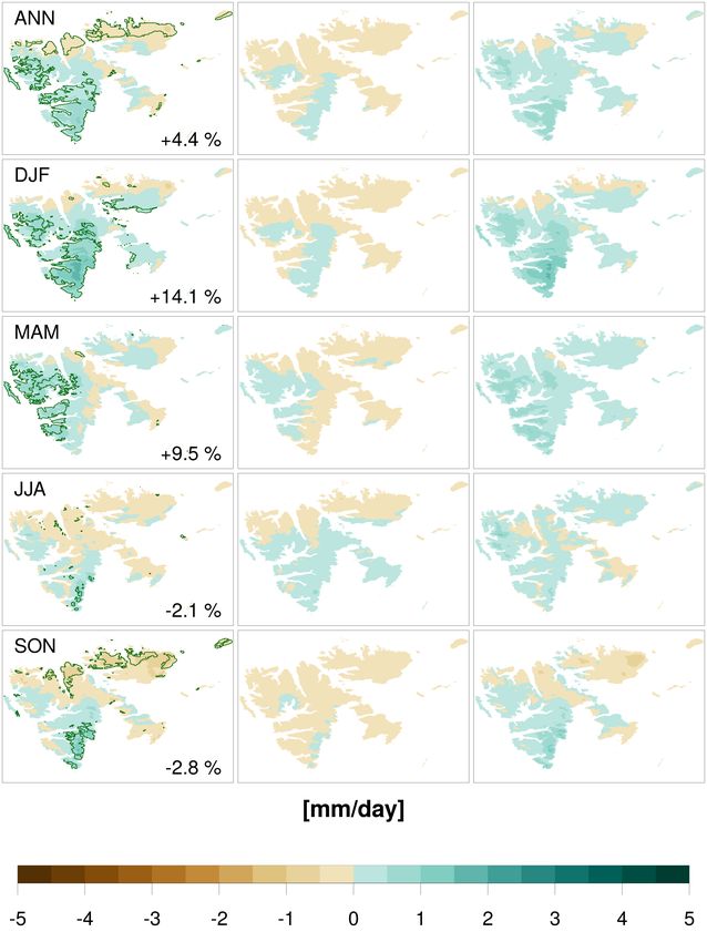
Atmosphere 2021, 11, 1378                                                                                       8 of 20

      Figure 5. Annual mean precipitation (top left) from the MPI-ESM-LR driven COSMO-CLM current
      climate (1971–2000) simulation and its decomposition into single weather types over Svalbard. For the
      annual mean, the average daily precipitation over the whole land area is shown in the bottom right
      corner. For the different weather types, the contribution to the total precipitation is given in the bottom
      right corner, while the number in the top left corresponds to the number of occurrences per year.

     Seasonal decompositions of the precipitation means are shown in the supporting material.
The patterns look similar for all seasons with some variations in the amplitude and spatial gradients.
Generally, the highest contributions to the overall precipitation are coming from autumn and winter
precipitation, followed by spring and summer.

3.1.4. Influence of the Driving Model
     An evaluation in [30] has shown that the biases in the MPI-ESM-LR driven COSMO-CLM
simulation for the current climate are similar to the ERA-Interim driven evaluation runs. Figure 6
shows that on average 4.4% more precipitation is simulated in the MPI-ESM-LR driven simulation.
More precipitation is falling in the southern part and less in the north. This pattern is similar for all
seasons with the largest differences in DJF (Figure 6). During JJA and SON, there is less precipitation
generated in the MPI-ESM-LR driven simulation, mostly due to lower precipitation values in the north.
However, especially for JJA, large parts of the differences are not statistically significant.
     Using formulas (1) and (2) (cf. Section 2.3) we can decompose the precipitation differences into
the parts coming from differences in the frequencies of the weather types and from differences in the
large-scale conditions. As shown in Figure 6, the precipitation differences are mostly due to differences
in the large-scale conditions. Assuming the mean large-scale conditions for each weather type in the
two models were equal, the resulting precipitation differences would be further reduced (shown in
the middle row of Figure 6). In other words, the contribution from the frequency mismatches is small.
However, especially for the northern area of Svalbard and in JJA, the frequency differences are partly
compensating the differences caused by the large-scale conditions.
Atmosphere 2021, 11, 1378 9 of 20
Figure 6. (Left): Difference between the annual and seasonal mean precipitation from the MPI-ESM-LR
and the ERA-Interim driven COSMO-CLM simulation for the current climate (1971–2000 and 2004–2017,
respectively). Statistically significant differences are outlined. (Center): The part resulting from
differences between the weather type frequencies in MPI-ESM-LR and ERA-Interim. (Right): The part
resulting from large-scale condition differences. The labels in the top left corners refer to the annual
mean (ANN) or the months of the specific season of the year.
3.2. Future Climate Projections
For the future climate projections, we are analysing the changes in the large-scale sea level pressure
and how they affect the COSMO-CLM precipitation. A special focus is directed to the heaviest daily
precipitation events.
3.2.1. Large-Scale Sea Level Pressure
Figure 7 shows that the mean annual sea level pressure decreases with about 0–2 hPa in the
future projections. Seasonally, the strongest signal can be seen in autumn which also shows the most
statistically significant changes. In winter, low pressure systems are projected to enter deeper into the
Kara sea. However, these changes are not statistically significant due to a strong annual variability.
Spring is the only season with a projected increase in sea level pressure, but the changes are only
statistically significant over Greenland and the high Arctic.Atmosphere 2021, 11, 1378 10 of 20
Figure 7. Projected changes from 1971–2000 to 2071–2100 in the mean annual and seasonal sea level
pressure in the MPI-ESM-LR climate simulation. Statistically significant changes are marked with dots.
The labels in the top left corners refer to the annual mean (ANN) or the months of the specific season
of the year.
Changes in the monthly frequencies of weather types in the future MPI-ESM-LR RCP8.5
projections relative to the historical simulations are presented in Figure 8. The changes in the
frequencies are small. Although there is a tendency to more pure cyclonic and less anticyclonic
situations in summer (and vice versa for the other seasons), there are only three statistically significant
changes: −1.9 pure cyclonic situations (Cc) in September, −1.8 Ec types in December and +0.3 Wa
types in October.
Figure 8. Mean monthly changes in the occurrence of weather types in the MPI-ESM-LR RCP8.5
projection (2071–2100) compared to the historical simulation (1971–2000). The dots mark statistically
significant changes.
The changes of sea level pressure for the single weather types (Figure 9) confirm that the low
pressure systems are entering deeper into the Kara sea, as already seen in the mean patterns (Figure 7).
Furthermore, the pressure pattern for SWc is becoming less north-south oriented. However, the changes
in the single patterns and the associated frequencies are small. Please note that on an annual scale,
none of the weather type frequency changes are statistically significant (not shown).Atmosphere 2021, 11, 1378 11 of 20
Figure 9. Annual mean sea level pressure from the future (2071–2100, in colours) and current (1971–2000,
as contour lines) MPI-ESM-LR simulation (top left) and the decomposition for single weather types.
The bold grey line shows the 1010 hPa level in the current climate and the dashed box the area used for
the weather type classification. In the top left corner, the number of events per year in the future and
current (in parentheses) simulation is given.
3.2.2. Local Precipitation
Figure 10 demonstrates the mean precipitation changes for the single weather types in the climate
projections. As can be seen, the total amount is increasing by 32.5%. There is an overall precipitation
increase in all weather types except SWa and Sa. Generally, the precipitation changes are highest and
statistically significant in the north-eastern part. In the south-western part, the changes are smallest
with a mostly non-significant decrease in precipitation projected for the weather types SWa and Sa.
Figures of the changes for the single weather types for all seasons are shown in the supplementary
materials. Generally, there is an increase for most weather types, but precipitation changes for the single
seasons and types vary. Local variations are especially apparent in winter for Nc and summer for SWc,
shown in Figure 11. For winter Nc conditions, a strong, statistically significant, precipitation increase
can be seen at the northern coast of Svalbard. There is also a decrease in precipitation projected in the
central region around Svalbard Airport but only a few points show statistically significant changes.
During summer SWc conditions, the model projects a decrease of precipitation on the windward
side of the mountains with statistically significant changes mostly in the Northern part. Considering
seasonal frequencies of weather types, there are only three cases of statistically significant changes
(see supplementary materials): Na in winter, NWa in spring and Ca in summer.Atmosphere 2021, 11, 1378 12 of 20
Figure 10. Annual mean precipitation change from 1971–2000 to 2071–2100 (top left) and its
decomposition into single weather types. Statistically significant changes are outlined. For the
annual mean, the number in the bottom right corner gives the mean increase. For the weather types,
the numbers give the contributions to the change and the contribution to the future mean precipitation
(in parentheses), respectively. In the top left corner, the frequencies (number of days per year) for the
future and current climate (in parentheses) are given.
Figure 11. Mean precipitation changes (from 1971–2000 to 2071–2100) for the weather type Nc in winter
(left) and SWc in summer (right). Statistically significant changes are outlined.
Weather type frequencies in the current and future climate, as well as their contribution to the
changes and the future mean precipitation are included in Figure 10. The largest contribution to the
changes are coming from the four cyclonic weather types Cc (19%), Ec (13%), NEc (12%) and SEc (9%).
In total, all cyclonic weather types contribute to about 74% of the changes, while the anticyclonic types
are summing up to 22% of the changes. Although Sc is contributing 6.5 % to the projected precipitationAtmosphere 2021, 11, 1378 13 of 20
in the future, its contribution to the change is only 2.8%. This can be explained by an even higher
contribution of 7.8% in the current climate (Figure 5). In contrast, the contribution from NEc to the
total precipitation is increasing from 4.4% to 6.2%. As the highest contribution (from Cc) is decreasing
and the lowest contribution (from NWa) is increasing, the contribution to the total precipitation from
the different weather types becomes more even.
On a seasonal scale, the largest overall increase can be seen in spring, followed by autumn,
winter and summer (Figure 12). Locally, the largest increases are projected for the northern and
northeastern parts in winter. Most of the projected changes are statistically significant with the
exception of summer and an area in the middle of the western parts of Svalbard. The decomposition
of the changes shows that they are almost completely due to changes in the large-scale conditions.
Summer is the exception, when changes due to frequencies are dominating. For the other seasons,
frequency changes alone would result in a general precipitation decrease. However, this is compensated
by the effects of the pronounced changes in large-scale conditions.
Figure 12. Changes in precipitation (from 1971–2000 to 2071–2100) decomposed into the contributions
from frequency and large-scale condition changes. (Left): Changes in the annual (top) and seasonal
mean precipitation climate projections over Svalbard. Statistically significant changes are outlined.
(Center): Precipitation changes resulting from frequency changes only. (Right): Differences resulting
from large-scale condition changes only.
3.2.3. Severe Weather Events
Figure 13 shows how the daily precipitation for the different weather types is changing in the
future projections. For all weather types, except Sa and SWa, the mean daily precipitation averaged
over Svalbard is increasing. For northerly and easterly flows, there is an increase of the contribution toAtmosphere 2021, 11, 1378 14 of 20
the total precipitation, while there is a decrease for southerly flows and Cc. The highest precipitation
values are projected to increase for all weather types except Ea, Ec and Wa, with the largest increases
for the northern advection types Nc and NEc.
Figure 13. Distributions for current (1971–2000, orange) and future (2071–2100, brown) mean daily
precipitation values over Svalbard associated with the different weather types. The crosses denote the
contribution to the total precipitation (in %) and the circles the mean precipitation (in mm/day) for
each weather type. The horizontal line in the box indicates the median, while bottom and top edges
indicate the first and third quartile, respectively. Whiskers extend to the most extreme value which is
no more than 1.5 times the interquartile range from the box. Data points outside the whisker range are
plotted as outliers. The width of the box indicates the number of events.
The highest values in the future projection are simulated under NEc, Cc and Nc conditions
(Figure 13). Simultaneously, the highest daily precipitation values under situations with air advection
from the south are increasing. For the western coast of Svalbard, where most settlements are located,
these conditions are often resulting in high precipitation amounts [4].
However, heavy precipitation at the west coast can also occur under other large-scale conditions.
As an illustration, Figure 14 shows sea level pressure and integrated water vapour (precipitable water)
in the atmosphere for the three highest precipitation amounts simulated at the approximate location
of Svalbard Airport in the COSMO-CLM simulations. The results show that the heavy precipitation
events are not dependant on a specific weather type. In all cases, there is advection of moist air towards
the west coast of Svalbard. For the third event in the current climate simulation however, the advection
of water vapour is caused by a local low pressure system west of Svalbard embedded in a larger
high-pressure system (i.e., a Ca situation) over Svalbard. For the future cases, a pronounced increase
in precipitable water can be seen. This is also apparent in the ten highest precipitation amounts
simulated (shown in the supplementary materials) indicating a possible reason for the projected
precipitation increases.Atmosphere 2021, 11, 1378 15 of 20
Figure 14. Precipitable water (colours) and sea level pressure (contours) for the top three precipitation
events in the 1971–2000 (left) and 2071–2100 (right) climate simulations. The labels in the top left
corner denote the corresponding weather type.
4. Discussion
For this study, the global climate model MPI-ESM-LR has been downscaled with COSMO-CLM to
2.5 km covering Svalbard for the time periods 1971–2000 and 2071–2100 following the RCP8.5 scenario.
A Jenkinson-Collison Types (JCT, [31]) classification has been performed, grouping atmospheric
circulation into 19 different weather types. The results of our analysis show a good agreement between
ERA-Interim and MPI-ESM-LR for weather type frequencies and mean sea level pressure patterns.
For Svalbard, a calendar of atmospheric circulation types has been developed by [35] based on a
method similar to the Lamb method [33]. The calendar provides a subjective weather type classification
(“Niedźwiedź classification”) and is available at http://www.kk.wnoz.us.edu.pl/nauka/kalendarz-
typow-cyrkulacji. In addition to the 19 JCT classes used here, the Niedźwiedź classification includes
a type for anticyclonic ridges and one for cyclonic troughs. Although an exact match of the weather
types from our analysis and the Niedźwiedź calendar cannot be expected, nor is it crucial to our
analysis, a comparison of the JCT statistics based on ERA-Interim data (Figure 3) and the Niedźwiedź
calendar (see e.g., [12]) shows that the JCT method is able to reproduce the Niedźwiedź classification
in a reasonable way but slightly favours the detection of pure cyclonic and anticyclonic situations.
The typical weather types for Svalbard [12] show varying spatial distributions of precipitation.
These patterns can generally be related to the conditions of the advected air. For Na, a high-pressure
system over eastern Greenland brings cold and dry air to Svalbard from the Arctic centre, resulting
in low precipitation values. For NEa, the situation is similar, but with a more tilted and southerly
low-pressure system, thus more dry air advection from the eastern Arctic area. In the Ea situation,
air masses are coming from the Siberian Arctic, resulting in generally dry conditions. However, for theAtmosphere 2021, 11, 1378 16 of 20
south-eastern tip of Svalbard, these situations can also bring some precipitation. The contribution to the
total precipitation from the frequently detected pure anticyclonic situation (Ca) over Svalbard is also
low, showing that the high-pressure situation results in very dry conditions generally. Notably, as our
analysis of the maximum daily precipitation events has shown, the Ca situation can nevertheless
result in heavy precipitation at the location of Svalbard Airport. This shows that there can be a
large variability within a single large-scale weather type due to local features. Thus, while the
average large-scale patterns and the associated precipitation fields provide a good overview of the
overall statistics, variations must be taken into account when looking at local and heavy precipitation
events. Under NEc conditions, low-pressure systems moving across Norway and reaching into the
Barents Sea are bringing some precipitation to the eastern coast. For Ec, occurring at about 37 days
a year, the low-pressure systems do not reach as deeply into the Barents Sea as for NEc, resulting in
precipitation falling mostly at the eastern coast of the southern tip. Although the differences between
cyclonic and anticyclonic mean weather patterns for a specific direction (e.g. NEc and NEa) can be
small, anticyclonic situations, usually associated with stable atmospheric conditions, are drier than the
corresponding cyclonic ones.
For the future climate, the MPI-ESM-LR projections show only small changes in the frequencies
and spatial patterns of weather types. However, for precipitation there is a significant increase projected
in the COSMO-CLM simulations with an increase for most weather types. The four weather types with
the highest contribution to the projected precipitation changes are Cc, Ec, NEc and SEc. None of these
are typically associated with moisture transport from lower latitudes, supporting the findings by [10]
that locally enhanced surface evaporation plays a major role in the increase of Arctic precipitation.
Specifically large precipitation changes are projected for the north-eastern parts during winter.
In this area, [18] have shown an ongoing warming and considered it likely that the area may become
largely ice-free in future winter conditions. This will result in a shifting of the now cold and continental
climate to a more maritime one, similar to the current climate in areas in the west. An effect of this
change will be an increased amount of precipitable water induced by evaporation over the ice-free
sea [40], which is reflected in the higher precipitation amounts in the northeast in our simulations.
Furthermore, [41] shows a positive correlation of sea-surface temperatures and water vapor for
the Nordic Seas and Kara Sea. Together with projected sea-surface temperatures warming in the
area [1], this will result in increased precipitable water and a possible contribution to the projected
precipitation changes.
A rather unexpected exception of the general precipitation increase are SWc conditions in summer.
Here, COSMO-CLM projects a decrease of precipitation on the western coast of Svalbard, i.e., the side
of the mountains oriented towards moisture advection. However, as pointed out by [42], the link
between increased Arctic precipitation and pole-ward moisture transport has not been constant or
straight forward in recent years. Although an enhanced moisture transport has been documented,
and can in general be assumed as a consequence of climate change [42], they did not find more moisture
provided for precipitation to the Arctic in summer, comparing the years after 2003 to those before.
Since our model results support these findings, it would be interesting to further investigate which
processes are weakening the link, but we leave this to future research.
The circulation patterns and frequencies derived from ERA-Interim and MPI-ESM-LR are
very similar, but COSMO-CLM produces some pronounced local precipitation variations for the
two driving models. Nevertheless, on average, the differences in the resulting precipitation
fields are small, pointing out that the MPI-ESM-LR model provides adequate boundary conditions
for the downscaling approach used in our study. To include more model uncertainty aspects,
a multi-model or multi-scenario ensemble of RCM simulations would have been the ideal set-up,
but simulations at kilometer scale are currently limited to smaller numbers due to their high
computational expense. However, comparing the COSMO-CLM simulations used in this study
with the Arctic-CORDEX regional climate model ensemble and empirical-statistically downscaled
global models, [1] demonstrates that the COSMO-CLM model shows relatively small changes but isAtmosphere 2021, 11, 1378 17 of 20
not a clear outlier. For the RCP8.5 emission scenario (used in this study), the Arctic-CORDEX ensemble
projects an increase in annual precipitation for Svalbard of about 27–106% with a median of 63%
from 1971–2000 to 2071–2100. COSMO-CLM projects a corresponding increase of 34%. For RCP4.5,
the Arctic-CORDEX RCMs project a lower, but still increasing precipitation amount of 22–53% with a
median of 43% [1].
We also analysed the frequencies of weather types in the CanESM2, NorESM1-M and EC-Earth
global models, which have been used as driving models within the Arctic-CORDEX framework [43].
The figures are shown in the Supplementary Materials. Similar to MPI-ESM-LR, the three other
models show a good representation of the ERA-Interim-based frequencies, and only a few significant
changes projected towards the end of the 21st century. This supports our findings that the frequencies
of weather types have only a small impact on the overall precipitation on Svalbard and further
suggests that the strong future warming in the area shown by [1] is unlikely to be due to changes
in weather type frequencies, but due to changes in the atmospheric conditions. To a certain extent,
the good representation and small changes of weather type frequencies may be an artefact of the global
models being tuned towards observed characteristics, but, as [12] have shown, also recent warming on
Svalbard can only be weakly associated with changes in weather type frequencies.
5. Conclusions
To adequately simulate local precipitation on Svalbard, a realistic representation of the large-scale
conditions in the Northern Atlantic is crucial. Based on an automated classification, our study
reveals a good representation of weather types in the global MPI-ESM-LR model. There are only a
few statistically significant differences in the frequencies of occurrences compared to ERA-Interim
reanalyses, mostly apparent in summer. Biases in the mean sea level pressure patterns for the
19 different weather types are small. Precipitation simulated by COSMO-CLM with boundary
conditions from MPI-ESM-LR and from ERA-Interim is similar. Overall we conclude that the
MPI-ESM-LR model provides realistic current climate boundary conditions for dynamical downscaling
experiments in the Svalbard area.
Comparing the past and future periods, we find only small changes in frequencies and mean
sea level pressure patterns of the weather types. At the same time, there is a pronounced increase in
precipitation on Svalbard, ranging from 14% in summer to 39% in spring. This indicates that neither
changes in weather type frequencies nor in sea level pressure can explain the changes in precipitation.
The decomposition method we used allows us to provide the contributions from changes in
frequencies and in atmospheric conditions of the different weather types in a quantitative matter.
In summary, the decomposition shows that precipitation changes are mostly due to changes in the
atmospheric conditions, while the contributions from changes in frequencies are small. Our results also
show that the contribution to the projected changes are non-uniformly distributed among the different
weather types and prevailing rotation. In total, changes under cyclonic weather types contribute to
about 74% of the precipitation changes, while the anticyclonic types are summing up to 22%.
Supplementary Materials: The following Figures are available online at http://www.mdpi.com/2073-4433/11/
12/1378/s1 , Figure S1: Mean sea level pressure biases in MPI-ESM-LR. Figures S2–S5: Seasonal precipitation for
the current climate simulation and the decomposition into weather types. Figures S6–S9: Seasonal precipitation
changes and the decomposition into weather types. Figure S10: Maps of precipitable water and sea level
pressure for the top ten precipitation events at Svalbard Airport in the current and future climate simulations.
Figures S11–S14: Mean monthly frequencies of weather types and their changes in different GCMs.
Author Contributions: Conceptualization, A.D. and J.L.; validation, A.D., J.L., O.L. and J.E.H.; methodology,
A.D. and O.L.; software, A.D. and O.L.; formal analysis, A.D., J.L., O.L. and J.E.H.; investigation, A.D., J.L., O.L.
and J.E.H.; resources, A.D., J.L., O.L. and J.E.H.; data curation, A.D.; writing—original draft preparation, A.D., J.L.,
O.L. and J.E.H.; writing—review and editing, A.D., J.L., O.L. and J.E.H.; visualization, J.L. and A.D.; supervision,
A.D. and J.E.H.; project administration, A.D.; funding acquisition, A.D. All authors have read and agreed to the
current version of the manuscript.
Funding: This research was funded by The Norwegian Environment Agency (Miljødirektoratet).Atmosphere 2021, 11, 1378 18 of 20
Acknowledgments: We acknowledge the CLM-Community and COSMO Consortium for provision of the
COSMO-CLM model and documentation. Computational resources for the COSMO-CLM simulations have
been provided by UNINETT Sigma2 - the National Infrastructure for High Performance Computing and Data
Storage in Norway. We acknowledge the European Centre for Medium-Range Weather Forecasts (ECMWF) for
the provision of ERA-Interim data. We want to thank the Arctic-CORDEX climate modelling groups for producing
and making available their model output data. For an easy access to the model data, we also acknowledge the
World Climate Research Programme’s Working Group on Regional Climate, and the Working Group on Coupled
Modelling, former coordinating body of CORDEX and responsible panel for CMIP5, as well as the Earth System
Grid Federation infrastructure, an international effort led by the U.S. Department of Energy’s Program for Climate
Model Diagnosis and Intercomparison, the European Network for Earth System Modelling and other partners
in the Global Organisation for Earth System Science Portals (GO-ESSP). We further thank Ketil Isaksen for his
valuable input to the manuscript and contribution to analyses that provided the basis of this article.
Conflicts of Interest: The authors declare no conflict of interest.
References
1. Hanssen-Bauer, I.; Førland, E.J.; Hisdal, H.; Mayer, S.; Sandø, A.B.; Sorteberg, A. Climate in Svalbard
2100—A knowledge base for climate adaptation. NCCS Rep. 2019, 1, 208. [CrossRef]
2. Larsson, S. Geomorphological Effects on the Slopes of Longyear Valley, Spitsbergen, After a Heavy Rainstorm
in July 1972. Geogr. Ann. Ser. A Phys. Geogr. 1982, 64, 105–125. [CrossRef]
3. Hansen, B.B.; Isaksen, K.; Benestad, R.E.; Kohler, J.; Pedersen, Å.Ø.; Loe, L.E.; Coulson, S.J.; Larsen, J.O.;
Varpe, Ø. Warmer and wetter winters: characteristics and implications of an extreme weather event in the
High Arctic. Environ. Res. Lett. 2014, 9, 114021. [CrossRef]
4. Dobler, A.; Førland, E.J.; Isaksen, K. Present and future heavy rainfall statistics for
Svalbard—Background-report for Climate in Svalbard 2100. NCCS Rep. 2019, 3, 29.
5. Serreze, M.C.; Crawford, A.D.; Barrett, A.P. Extreme daily precipitation events at Spitsbergen, an Arctic
Island. Int. J. Climatol. 2015, 35, 4574–4588. [CrossRef]
6. Osuch, M.; Wawrzyniak, T. Climate projections in the Hornsund area, Southern Spitsbergen. Pol. Polar Res.
2016, 37, 379–402. [CrossRef]
7. AMAP. Snow, Water, Ice and Permafrost in the Arctic (SWIPA) 2017; Arctic Monitoring and Assessment
Programme (AMAP): Oslo, Norway, 2017.
8. Kattsov, V.M.; Walsh, J.E.; Chapman, W.L.; Govorkova, V.A.; Pavlova, T.V.; Zhang, X. Simulation
and Projection of Arctic Freshwater Budget Components by the IPCC AR4 Global Climate Models.
J. Hydrometeorol. 2007, 8, 571–589. [CrossRef]
9. Bengtsson, L.; Hodges, K.I.; Koumoutsaris, S.; Zahn, M.; Keenlyside, N. The changing atmospheric water
cycle in Polar Regions in a warmer climate. Tellus A Dyn. Meteorol. Oceanogr. 2011, 63, 907–920. [CrossRef]
10. Bintanja, R.; Selten, F.M. Future increases in Arctic precipitation linked to local evaporation and sea-ice
retreat. Nature 2014, 509, 479–482. [CrossRef]
11. Hanssen-Bauer, I.; Førland, E. Long-term trends in precipitation and temperature in the Norwegian Arctic:
can they be explained by changes in atmospheric circulation patterns? Clim. Res. 1998, 10, 143–153.
[CrossRef]
12. Isaksen, K.; Nordli, Ø.; Førland, E.J.; Łupikasza, E.; Eastwood, S.; Niedźwiedź, T. Recent warming on
Spitsbergen—Influence of atmospheric circulation and sea ice cover. J. Geophys. Res. Atmos. 2016, 121, 11–913.
[CrossRef]
13. Dahlke, S.; Maturilli, M. Contribution of Atmospheric Advection to the Amplified Winter Warming in the
Arctic North Atlantic Region. Adv. Meteorol. 2017, 2017, 1–8. [CrossRef]
14. Meinshausen, M.; Smith, S.J.; Calvin, K.; Daniel, J.S.; Kainuma, M.L.T.; Lamarque, J.F.; Matsumoto, K.;
Montzka, S.A.; Raper, S.C.B.; Riahi, K.; et al. The RCP greenhouse gas concentrations and their extensions
from 1765 to 2300. Clim. Chang. 2011, 109, 213–241. [CrossRef]
15. Gjelten, H.M.; Nordli, Ø.; Isaksen, K.; Førland, E.J.; Sviashchennikov, P.N.; Wyszynski, P.; Prokhorova, U.V.;
Przybylak, R.; Ivanov, B.V.; Urazgildeeva, A.V. Air temperature variations and gradients along the coast and
fjords of western Spitsbergen. Polar Res. 2016, 35, 29878. [CrossRef]
16. Nordli, Ø.; Przybylak, R.; Ogilvie, A.E.; Isaksen, K. Long-term temperature trends and variability on
Spitsbergen: the extended Svalbard Airport temperature series, 1898–2012. Polar Res. 2014, 33, 21349.
[CrossRef]Atmosphere 2021, 11, 1378 19 of 20
17. Osuch, M.; Wawrzyniak, T. Inter- and intra-annual changes in air temperature and precipitation in western
Spitsbergen. Int. J. Climatol. 2016, 37, 3082–3097. [CrossRef]
18. Dahlke, S.; Hughes, N.E.; Wagner, P.M.; Gerland, S.; Wawrzyniak, T.; Ivanov, B.; Maturilli, M. The observed
recent surface air temperature development across Svalbard and concurring footprints in local sea ice cover.
Int. J. Climatol. 2020, 40, 5246–5265. [CrossRef]
19. Lind, P.; Belušić, D.; Christensen, O.B.; Dobler, A.; Kjellström, E.; Landgren, O.; Lindstedt, D.; Matte, D.;
Pedersen, R.A.; Toivonen, E.; Wang, F. Benefits and added value of convection-permitting climate modeling
over Fenno-Scandinavia. Clim. Dyn. 2020, 55, 1893–1912. [CrossRef]
20. Pontoppidan, M.; Reuder, J.; Mayer, S.; Kolstad, E.W. Downscaling an intense precipitation event in complex
terrain: the importance of high grid resolution. Tellus A Dyn. Meteorol. Oceanogr. 2017, 69, 1271561.
[CrossRef]
21. Prein, A.F.; Langhans, W.; Fosser, G.; Ferrone, A.; Ban, N.; Goergen, K.; Keller, M.; Tölle, M.; Gutjahr, O.;
Feser, F.; et al. A review on regional convection-permitting climate modeling: Demonstrations, prospects,
and challenges. Rev. Geophys. 2015, 53, 323–361. [CrossRef]
22. Früh, B.; Will, A.; Castro, C.L. Editorial: Recent developments in Regional Climate Modelling with
COSMO-CLM. Meteorol. Z. 2016, 25, 119–120. [CrossRef]
23. Jacob, D.; Petersen, J.; Eggert, B.; Alias, A.; Christensen, O.B.; Bouwer, L.M.; Braun, A.; Colette, A.; Déqué,
M.; Georgievski, G.; et al. EURO-CORDEX: new high-resolution climate change projections for European
impact research. Reg. Environ. Chang. 2013, 14, 563–578. [CrossRef]
24. Kotlarski, S.; Keuler, K.; Christensen, O.B.; Colette, A.; Déqué, M.; Gobiet, A.; Goergen, K.; Jacob, D.; Lüthi, D.;
van Meijgaard, E.; et al. Regional climate modeling on European scales: a joint standard evaluation of the
EURO-CORDEX RCM ensemble. Geosci. Model Dev. 2014, 7, 1297–1333. [CrossRef]
25. Kessler, E. On the continuity and distribution of water substance in atmospheric circulations. Atmos. Res.
1995, 38, 109–145. [CrossRef]
26. Ritter, B.; Geleyn, J.F. A Comprehensive Radiation Scheme for Numerical Weather Prediction Models with
Potential Applications in Climate Simulations. Mon. Weather. Rev. 1992, 120, 303–325. [CrossRef]
27. Dee, D.P.; Uppala, S.M.; Simmons, A.J.; Berrisford, P.; Poli, P.; Kobayashi, S.; Andrae, U.; Balmaseda, M.A.;
Balsamo, G.; Bauer, P.; et al. The ERA-Interim reanalysis: configuration and performance of the data
assimilation system. Q. J. R. Meteorol. Soc. 2011, 137, 553–597. [CrossRef]
28. Giorgetta, M.A.; Jungclaus, J.; Reick, C.H.; Legutke, S.; Bader, J.; Böttinger, M.; Brovkin, V.; Crueger, T.;
Esch, M.; Fieg, K.; et al. Climate and carbon cycle changes from 1850 to 2100 in MPI-ESM simulations for the
Coupled Model Intercomparison Project phase 5. J. Adv. Model. Earth Syst. 2013, 5, 572–597. [CrossRef]
29. Brisson, E.; Demuzere, M.; van Lipzig, N.P. Modelling strategies for performing convection-permitting
climate simulations. Meteorol. Z. 2016, 25, 149–163. [CrossRef]
30. Dobler, A. Convection permitting climate simulations for Svalbard—Background-report for Climate in
Svalbard 2100. NCCS Rep. 2019, 2, 27.
31. Jenkinson, A.; Collison, F. An initial climatology of gales over the North Sea. Synop. Climatol. Branch Memo.
1977, 62, 18. Available online: https://library.metoffice.gov.uk/Portal/Default/enGB/RecordView/Index/
175564 (accessed on 18 December 2020).
32. Jones, P.D.; Hulme, M.; Briffa, K.R. A comparison of Lamb circulation types with an objective classification
scheme. Int. J. Climatol. 1993, 13, 655–663. [CrossRef]
33. Lamb, H.H. British Isles weather types and a register of the daily sequence of circulation patterns 1861–1971.
Geophys. Mem. 1972, 116,1861–1971.
34. Jones, P.D.; Harpham, C.; Briffa, K.R. Lamb weather types derived from reanalysis products. Int. J. Climatol.
2012, 33, 1129–1139. [CrossRef]
35. Niedźwiedź, T. Climate and Climate Change at Hornsund, Svalbard; Marsz, A.A., Styszyńska, A., Eds.;
Gdynia Maritime University: Gdyni, Poland, 2013.
36. Huth, R.; Beck, C.; Philipp, A.; Demuzere, M.; Ustrnul, Z.; Cahynová, M.; Kyselý, J.; Tveito, O.E.
Classifications of Atmospheric Circulation Patterns. Ann. N. Y. Acad. Sci. 2008, 1146, 105–152. [CrossRef]
[PubMed]
37. Smirnov, N. Table for estimating the goodness of fit of empirical distributions. Ann. Math. Stat. 1948,
19, 279–281. [CrossRef]Atmosphere 2021, 11, 1378 20 of 20
38. Koenigk, T.; Berg, P.; Döscher, R. Arctic climate change in an ensemble of regional CORDEX simulations.
Polar Res. 2015, 34, 24603. [CrossRef]
39. Isaksen, K.; Førland, E.J.; Dobler, A.; Benestad, R.; Haugen, J.E.; Mezghani, A. Klimascenarioer for
Longyearbyen-området, Svalbard. MET Nor. Rep. 2017, 14, 2017.
40. Rinke, A.; Segger, B.; Crewell, S.; Maturilli, M.; Naakka, T.; Nygård, T.; Vihma, T.; Alshawaf, F.; Dick, G.;
Wickert, J.; et al. Trends of Vertically Integrated Water Vapor over the Arctic during 1979–2016: Consistent
Moistening All Over? J. Clim. 2019, 32, 6097–6116. [CrossRef]
41. Carvalho, K.; Wang, S. Sea surface temperature variability in the Arctic Ocean and its marginal seas in a
changing climate: Patterns and mechanisms. Glob. Planet. Chang. 2020, 193, 103265. [CrossRef]
42. Gimeno-Sotelo, L.; Nieto, R.; Vázquez, M.; Gimeno, L. A new pattern of the moisture transport for
precipitation related to the drastic decline in Arctic sea ice extent. Earth Syst. Dyn. 2018, 9, 611–625.
[CrossRef]
43. Akperov, M.; Rinke, A.; Mokhov, I.I.; Semenov, V.A.; Parfenova, M.R.; Matthes, H.; Adakudlu, M.; Boberg, F.;
Christensen, J.H.; Dembitskaya, M.A.; et al. Future projections of cyclone activity in the Arctic for the 21st
century from regional climate models (Arctic-CORDEX). Glob. Planet. Chang. 2019, 182, 103005. [CrossRef]
Publisher’s Note: MDPI stays neutral with regard to jurisdictional claims in published maps and institutional
affiliations.
© 2020 by the authors. Licensee MDPI, Basel, Switzerland. This article is an open access
article distributed under the terms and conditions of the Creative Commons Attribution
(CC BY) license (http://creativecommons.org/licenses/by/4.0/).You can also read