Solar large-scale magnetic field and cycle patterns in solar dynamo - arXiv.org
←
→
Page content transcription
If your browser does not render page correctly, please read the page content below
MNRAS 000, 000–000 (0000)                            Preprint 16 April 2021              Compiled using MNRAS LATEX style file v3.0

                                               Solar large-scale magnetic field and cycle patterns in solar
                                               dynamo
                                               V.N. Obridko1 , ? , V. Pipin4 †, D. Sokoloff1,2,3 ‡, A.S. Shibalova2,3 ,§
                                               1 IZMIRAN,     4 Kaluzhskoe Shosse, Troitsk, Moscow, 108840
                                               2 Department    of Physics, Moscow State University, Moscow,119992, Russia
                                               3 Moscow Center of Fundamental and Applied Mathematics, Moscow, 119991, Russia
                                               4 Institute of Solar-Terrestrial Physics, Russian Academy of Sciences, Irkutsk, 664033, Russia
arXiv:2104.06808v2 [astro-ph.SR] 15 Apr 2021

                                               16 April 2021

                                               ABSTRACT
                                               We compare spectra of the zonal harmonics of the large-scale magnetic field of the Sun using observation results
                                               and solar dynamo models. The main solar activity cycle as recorded in these tracers is a much more complicated
                                               phenomenon than the eigen solution of solar dynamo equations with the growth saturated by a back reaction of the
                                               dynamo-driven magnetic field on solar hydrodynamics. The nominal 11(22)-year cycle as recorded in each mode has
                                               a specific phase shift varying from cycle to cycle; the actual length of the cycle varies from one cycle to another and
                                               from tracer to tracer. Both the observation and the dynamo model show an exceptional role of the axisymmetric `5
                                               mode. Its origin seems to be readily connected with the formation and evolution of sunspots on the solar surface.
                                               The results of observations and dynamo models show a good agreement for the low `1 and `3 modes. The results for
                                               these modes do not differ significantly for the axisymmetric and nonaxisymmetric models. Our findings support the
                                               idea that the sources of the solar dynamo arise as a result of both the distributed dynamo processes in the bulk of
                                               the convection zone and the surface magnetic activity.
                                               Key words: Sun: magnetic fields; Sun: oscillations; sunspots

                                               1 INTRODUCTION                                                       activity (sunspots, flares, filaments, corona, solar wind, etc.)
                                                                                                                    are addressed in many papers (see for review, e.g., Hathaway
                                               Until the middle of the past century, the solar activity was
                                                                                                                    2015, Usoskin 2017).
                                               considered mainly as a periodic modulation of sunspot num-
                                                                                                                       Here, we concentrate our analysis on the structure of the
                                               bers. This viewpoint survives even now among people not
                                                                                                                    large-scale global magnetic field presented as a combination
                                               closely related to solar astronomy. In fact, however, the so-
                                                                                                                    of multi-poles of various order. We are interested in the time
                                               lar activity is a complex of interconnected physical processes
                                                                                                                    evolution of individual multi-poles as well as their correla-
                                               mainly underlied by magnetic field variations. The variety of
                                                                                                                    tions. The amplitudes and phases of the lowest multipoles and
                                               physical processes included in solar activity is determined by
                                                                                                                    their correlations with the solar photospheric magnetic field
                                               the fact that the solar magnetic field contains various compo-
                                                                                                                    have been investigated in various papers (e.g., Levine 1977;
                                               nents and is produced by several drivers, such as, e.g., the dif-
                                                                                                                    Hoeksema 1984; Stenflo & Vogel 1986; Stenflo & Weisen-
                                               ferential rotation, meridional circulation, and the turbulent
                                                                                                                    horn 1987; Hoeksema 1991; Levine 1977; Gokhale et al. 1992;
                                               dynamo effects. The differential rotation of the Sun is well
                                                                                                                    Gokhale & Javaraiah 1992; Stenflo 1994; Knaack & Stenflo
                                               known thanks to the helioseismology results (see, e.g. Howe
                                                                                                                    2005) on the basis of Kitt Peak and WSO (John Wilcox Ob-
                                               et al. 2011). The parameters of meridional circulation are de-
                                                                                                                    servatory, Stanford) data.
                                               batable (see, e.g, the recent discussion in Gizon et al. 2020
                                               and Stejko et al. 2021 and references therein). Our knowl-              We will focus on higher-order axisymmetric multipoles in
                                               edge of the turbulent dynamo effects is even more uncertain          order to determine the number l, which gives the main con-
                                               Brandenburg (2018). The spacial and temporal magnetic field          tribution to the spectrum of the large-scale magnetic field.
                                               variations are important to understand the very origin of the        We believe that such a research is interesting in itself, as well
                                               solar magnetic field as well as its relation to the solar activ-     as in the context of comparison with solar dynamo models.
                                               ity manifestations. Magnetic fields in various objects of solar      Now the most popular kind of the solar dynamo, which suc-
                                                                                                                    cessfully reproduces many observational facts concerning the
                                                                                                                    solar activity is the Babcock-Leighton scheme (e.g., Char-
                                                                                                                    bonneau 2020). The polar magnetic field remaining from the
                                               ? email:obridko@izmiran.ru
                                               † email: pip@iszf.irk.ru                                             previous cycle changes its sing during the sunspot number
                                               ‡ email: sokoloff.dd@gmail.com                                       growth phase (Wang et al. 1989, Benevolenskaya 2004, Dasi-
                                               § email:as.shibalova@physics.msu.ru                                  Espuig et al. 2010).

                                               © 0000 The Authors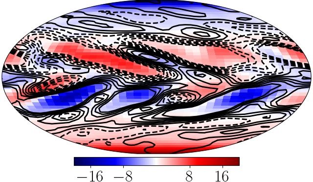
2 V.N. Obridko, V.V. Pipin, D.D. Sokoloff, A.S. Shibalova
Earlier, DeRosa et al. (2012) found that the coupling be- ingly; Plm are the associated Legendre polynomials; glm and
tween the odd and even (anti-symmetric & symmetric about hlm are the Gauss coefficients calculated under the assump-
the equator) modes shows a correlation with the large-scale tion that the magnetic field is potential between the photo-
polarity reversals both in observations and in the Babcock- sphere and the source surface, while the magnetic field is pre-
Leighton type dynamo models. The results obtained by Pas- sumed to be exactly radial at the source surface. We do not
sos et al. (2014) and Hazra et al. (2014), as well as the up- include the correction coefficient 1.8 suggested by Svalgaard
dated version of the Babcock-Leighton dynamo model pre- et al. (1978); however, it is more than possible to re-scale the
sented in Cameron & Schüssler (2017) show that the poloidal results below including this coefficient. The harmonic coeffi-
magnetic field can be generated in the solar dynamo by two cients are generated on the base of the summary year-long
different sources. One is related to the surface evolution of synoptic map for every rotation with the cadence equal to
the tilted bipolar regions and the other comes from turbu- half a Carrington rotation.
lent generation of the poloidal magnetic field from the large- Following Obridko et al. (2020), we obtain the Gauss coef-
scale toroidal field by the α-effect in the bulk of the con- ficients glm and hlm independently rather than just defining
vection zone. The latter source is a usual component in the their ratio. Then, following Obridko & Yermakov (1989), we
distributed mean-field dynamo models. Note that the dis- average Eqs. 1 over the photosphere and the source surface,
tributed dynamo paradigm is supported by a number of the respectively to yield
global convection simulation models (see, e.g., Käpylä et al. X (l + 1 + lζ 2l+1 ) 2
2016; Warnecke et al. 2018). A comparison of the distributed < Br2 >|R0 = (glm + h2lm ), (4)
dynamo model and the Babcock-Leghton scenario can be 2l + 1
lm
found in (Brandenburg 2005; Kosovichev et al. 2013).
X
< Br2 >|Rs = (2l + 1)ζ 2l+4 (glm
2
+ h2lm ), (5)
In this paper, we aim to investigate the relative contribu- lm
tion of the dynamo in the depth of the convection zone and
the surface sunspot activity to the evolution of the axisym- where ζ = R0 /Rs and < ... > stands for averaging. < Br2 > is
metric modes. The main idea is to study the phase relation the mean square radial component of the magnetic field cal-
between the evolution of different ` modes at the surface and culated by formula (1). Since the polynomials are orthonor-
to compare the results of observations with the results of the mal, the integration can be done analytically. Integration can
dynamo models. The phase relation between the mode evo- be performed over any spherical surface by substituting the
lution was previously studied by Stenflo (1994) and Knaack required value of R. In this case, the formulas are given for
& Stenflo (2005). They found an exceptional role of the ax- the photosphere surface (4) and the source surface (5). This
isymmetric harmonic ` = 5. DeRosa et al. (2012) analyzed the means that the contribution of the lth mode to the average
phase relations between the low ` harmonics in the Babcock- magnetic field contains an l-dependent coefficient. Compar-
Leighton type dynamo and revealed nearly synchronous evo- ing the relative contributions of modes with various l we plot
lution of the ` = 1, 3 and ` = 5 (see Fig. 15 in DeRosa square roots of contribution with given l in Eqs. (4 - 5).
et al. (2012)). This seems to contradict the results by Stenflo Of course, we use for comparison more traditional solar
(1994). Here, we intend to repeat the analysis using observa- activity data like sunspots where required.
tional data from the Wilcox Solar Observatory.
.
3 OBSERVATIONAL RESULTS: AXIAL
SYMMETRY AND PARITY OF THE
2 OBSERVATIONAL BASIS AND BASIC L-HARMONICS
EQUATIONS 3.1 l-parity
We have been working with the WSO (Stanford University) The solar magnetic field is traditionally claimed as a magnetic
synoptic maps of the light-of-sight photospheric magnetic field of dipole symmetry, i.e., antisymmetric in respect to
field component (Scherrer et al. 1977) for the period from the solar equator. The most straightforward representation of
Carrington rotation 1642 (beginning on 27 May 1976) till ro- such view is the famous Hale polarity law of sunspot groups.
tation 2227 (beginning on 2 February 2020) converted into Of course, the dipole symmetry is not perfect and various
Gaussian coefficients using the standard expressions deviations are known.
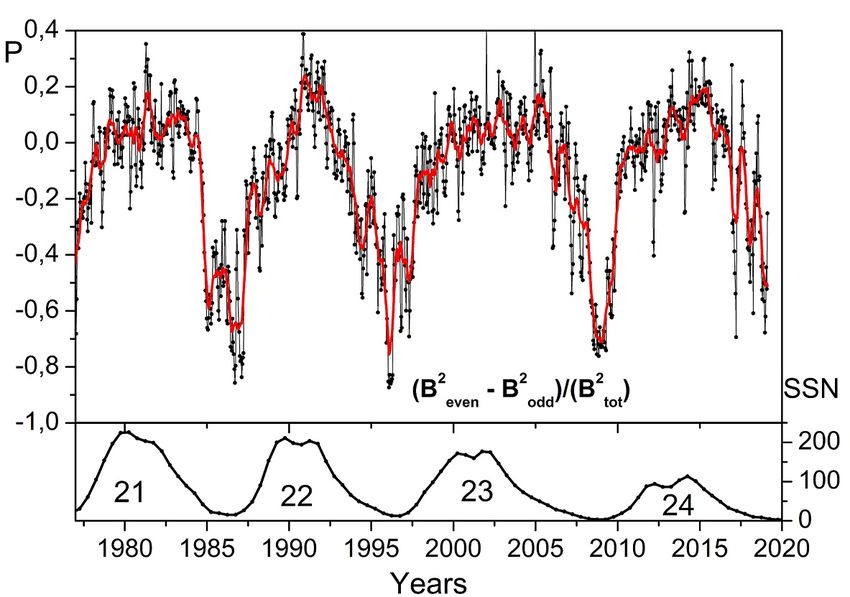
X m Fig.1 (top panel) represents the contribution of various l-
Br = Pl (cos θ)(glm cos mφ + hlm sin mφ) × (1)
harmonics to the mean surface magnetic field versus time.
l,m
Some prevalence of the even harmonics is visible. The integral
×((l + 1)(R0 /R)l+2 − l(R/Rs )l−1 cl ), parameter, which characterizes the equatorial symmetry of
X ∂P m (cos θ) the large-scale magnetic field, is given by the parity index,
l
Bθ = − (glm cos mφ + (2)
∂θ 2 2 2 2
l,m P = (Beven − Bodd )/(Beven + Bodd ). (6)
l+2 l−1
+hlm sin mφ)((R0 /R) + (R/Rs ) cl ), It reflects the relative power of the odd and even harmonics
X m m
Bφ = − Pl (cos θ)(hlm cos mφ − (3) in the energy of the large-scale magnetic field. The negative
sin θ values correspond to the equatorial anti-symmetry (−1 - the
l,m
dipole parity) and the positive values, to the symmetry (+1
−glm sin mφ)((R0 /r)l+2 + (R/Rs )l−1 cl ).
- the quadrupole parity). This parameter is commonly used
Here, 0 ≤ m ≤ l < N , cl = −(R0 /Rs )l+2 , R0 , and Rs are the in solar dynamo models (Brandenburg et al. 1989; Knobloch
radii of the solar surface and the sours surface, correspond- et al. 1998; Weiss & Tobias 2016). From Fig.1 (middle), we
MNRAS 000, 000–000 (0000)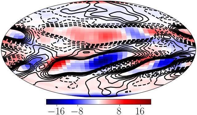
Solar large-scale magnetic field and cycle patterns in solar dynamo                               3

Figure 1. Top panel – contribution of each of the first 20 har-
monics (l = 0, 1, 2, ..., 19) on the photosphere surface to the mean   Figure 2. Contribution of each of the first 20 axisymmetric har-
magnetic field versus time. The middle shows the parity index, P,      monics (l = 0, 1, 2, ..., 19) to the mean magnetic field on the pho-
where the black curves show the raw data; each dot corresponds         tosphere surface versus time, m = 0 (top); relative contribution
to half a Carrington rotation, and the red curve represent 13-point    of nonaxisymmetric harmonics (m 6= 0) to the mean square mag-
smoothing. The bottom shows the solar cycle according to sunspot       netic field on the photosphere surface versus time (middle); and
data.                                                                  total contribution of nonaxisymmetric harmonics to the mean so-
                                                                       lar magnetic field (bottom). The blue curve on the lower panel
                                                                       shows the solar cycle according to sunspot data.

see that the solar dynamo shows the dipole-type symmetry
during the solar minimum. The solar maximum is charac-                       0,6
terized by the magnetic field distribution highly asymmetric
about the equator. Later, we shall discuss the origin of this                0,4
phenomenon in more detail.
                                                                             0,2
                                                                       [G]

                                                                             0,0
3.2 Axisymmetric versus non-axisymmetric
    harmonics                                                                -0,2
It is interesting that the evolution of the ` parity of the solar                                           g10
magnetic field seems to be related to the parameters of the ax-              -0,4
ial symmetry. Fig. 2 (top) shows the evolution of the ` power                                               g30          g70
for the axisymmetric modes of the solar magnetic field during                -0,6                           g50          g20
the past four solar cycles. We see its substantial decreases at
the end of the observational epoch. This indicates that so-                         1980     1990         2000          2010         2020
lar activity has declined substantially in the past two cycles                                      t, years
as compared to the end of the XX century. The integral pa-
rameter characterizing the relative power of nonaxisymmet-             Figure 3. The smoothed series of the first 4 odd axisymmetric
ric harmonics follows the evolution of the sunspot activity.           harmonics together with he lowest even axisymmetric harmonic.
This parameter is close to unity during the maximum of the             The data averaged by convolution with the Gaussian function (pa-
sunspot activity (cf, Vidotto et al. 2018). The solar minima           rameter σ = 0.75).
show a predominance of the axisymmetric harmonics.

                                                                                                            MNRAS 000, 000–000 (0000)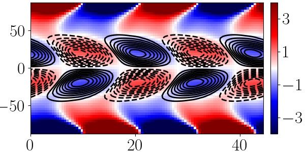
4     V.N. Obridko, V.V. Pipin, D.D. Sokoloff, A.S. Shibalova

Table 1. Phase shifts of the first axisymmetric harmonics with
                                                                        0,5
                                                                                    SN
the odd numbers juxtaposed with the phase of the solar cycle as
inferred from the polar magnetic field and sunspot data. We have                    Bpol
chosen the phase of g50 = 0. The correlation functions (except          0,4
                                                                                       1
the one for sunspots) have two maxima and, correspondingly, two
estimates of the phase shift. The estimate corresponding to the                        3
main maximum of the correlation function is given as the basic          0,3
value and the other value is added in brackets. The discrepancy                        5

                                                                    S
between the main quantities and the estimates given in brackets
provide us with additional option for measuring the accuracy of         0,2            7
the estimates.

                             ∆t, years            φ
                                                                        0,1
              g10         −2.28 (−2.03)     0.23π (0.20π)
                                                                        0,0
              g30         −2.69 (−2.29)     0.27π (0.23π)
                                                                      a)
              g50                0                0                           0            5               10          15              20
                                                                                                    ∆t, Yr
              g70         −3.69 (−3.11)     0.37π (0.31π)                         -8           -4            0     4          8
                                                                              r
            Bpolar        −1.91 (−0.97)     0.19π (0.10π)
                                                                         1,0                                                5,Bpol
       Sunspot number          3.29            −0.33π
                                                                                                                            5,SN
                                                                         0,5
4 CYCLICITY IN AXISYMMETRIC
  HARMONICS
                                                                         0,0
The analysis of the cyclic behavior of axisymmetric modes has
run into some difficulties. As seen from Fig. 2, not only the
even axisymmetric harmonics, but also the higher-order odd              -0,5                         5,1
ones yield a chaotic, unrealistic picture. Apparently, taking                                        5,3
into account any harmonics of the order higher than l =
                                                                        -1,0                         5,5
7 results in violation of the regular cyclic dependence (see,
Hoeksema 1995, http://wso.stanford.edu/Polar.html).                                                  5,7
                                                                        b)
   Then, we search for harmonics with a pronounced cyclic be-                                  /2            0      - /2           -
havior and select four such harmonics, namely, g10 , g30 , g50 ,
and g70 , Fig. 3. We do not see pronounced cyclicity in ax-         Figure 4. a) Integral wavelet spectra for several odd harmonics,
                                                                    the strength of the polar magnetic field and the SN index; b) Cor-
isymmetric harmonics with the even numbers; however, they
                                                                    relation coefficients r between g50 and the other tracers of solar
are interesting as indicators of the North-South asymmetry
                                                                    activity under discussion (g10 - red, g30 - blue, g50 - black, and
DeRosa et al. 2012. To be specific, the red dashed line in Fig. 3   g70 - light green) in comparison with the polar field Bpolar (purple
show the lowest harmonic g20 . Despite the activity of g20 is       dashed) and sunspots (dark green). The phase of the cycle is given
irregular it shows a correlation with the polar field reversals     in years (upper horizontal scale) in phase φ of the whole cycle,
(DeRosa et al. 2012). Fig. 3 shows a phase difference in the        which is 2π.
evolution of the odd axisymmetric harmonics. This difference
was analyzed by Stenflo (1994). He found, in particular, that
an extended solar cycle in the evolution of the radial mag-         quite arbitrarily the harmonic g50 as the basic one. More
netic field can inherently result from the evolution of modes,      specifically, we consider two signals, say, f (t) and g(t), shift
which follows some phase relations. Therefore, the phase re-        signal g in time by ∆t, and calculate the correlation function
lations can shed light on the origin of the solar dynamo. The       r. The result is plotted in Fig. 4b as a function of ∆t. For
analysis of Stenflo (1994) was based on the assumption of a         comparison with Stenflo (1994), we have chosen the phase of
unique period for the axisymmetric modes. Here we consider          g50 equal to 0. Therefore, the mode g50 in Fig 4b is shown
a more general situation.                                           by the auto-correlation coefficient. In order to compare with
   Fig. 4a shows the integral wavelet spectra for the low odd       the above-cited paper, we have to take into account that the
harmonics, the strength of the polar magnetic field and the         highest correlation is attained by shifting the advance har-
SN index. The cycle lengths of the modes, as well as the            monic backward or by shifting the lagged harmonic forward.
corresponding quantities for the polar filed and the sunspot        Therefore, the signs for the time and phase are opposite. Sim-
numbers determined as the location of the maxims in the             ilarly to Stenflo (1994) we find the positive sign for the phase
integral wavelet spectra. They are given in Table 2. One can        shifts of the all harmonics. Though the magnitude of the shift
see, that the different parameters show the different cycle         is about factor twice less than in his study. Recall that r is
length. Notably, The parameter g50 shows the smallest period        a dimensionless quantity and |r| ≤ 1. The location of maxi-
of about 10 years.                                                  mum r for the particular tracer of the solar activity is used as
   In order to obtain the phase shift between the axisymmet-        the phase shift of the tracer in respect to the mode g50 . The
ric harmonics and some other tracers of solar activity, we          autocorrelation coefficient for g50 is also shown in the figure
calculate the corresponding correlation coefficients choosing       for comparison.

MNRAS 000, 000–000 (0000)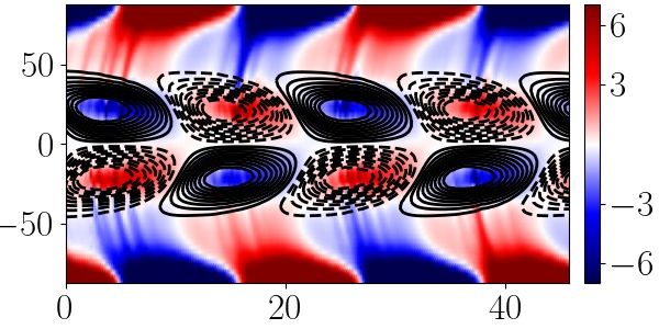
Solar large-scale magnetic field and cycle patterns in solar dynamo                      5

Table 2. Cycle lengths of the modes under discussion, polar mag-    5 RESULTS FROM MEAN-FIELD DYNAMO
netic field, and sunspot numbers: T is the cycle length for the       MODELS
absolute value, Ts is the cycle length for the signed quantities.
                                                                    In a preliminary study we considered the results of the run C2
                               T (years)    Ts (years)              from the axisymmetric dynamo model of Pipin & Kosovichev
                                                                    (2020). A detailed description of the model is given in the
                  g10            11.5         23.0                  above-cited paper. Note that the model explains successfully
                  g30            11.75        23.5                  the so-called “extended” solar cycle (Altrock (1997)) and, be-
                                                                    sides that, it shows a satisfactory agreement with many as-
                  g50            9.75         19.5                  pects of solar observations. However, that model does not
                  g70           11.625        23.25                 take into account the effect of the sunspot activity on the
                                                                    evolution of the radial magnetic field. Despite this, it shows
                Bpolar           10.5         21.0                  a satisfactory agreement of evolution of the low ` modes with
           Sunspot number        11.0         22.0                  observations. We provide these results in Appendix B. This
                                                                    model will be a reference in our study of the relative con-
                                                                    tributions of the deep and surface dynamo processes to the
                                                                    whole magnetic variability of the Sun. To study the possible
                                                                    effects of the sunspot activity on the dynamo evolution, we
   Note that the maximum values of r are quite high exceed-         consider the nonaxisymmetric dynamo model.
ing 0.9 for g10 and g30 , and even the lowest value (obtained for      We assume that the toroidal magnetic field in the subsur-
sunspots) exceeds 0.7. The fact that correlations between the       face layer of the convection zone is responsible for the forma-
harmonics of the large-scale poloidal magnetic field are larger     tion of solar bipolar regions in the photosphere. The effect
than their correlations with the polar magnetic field and the       of inclination of the bipolar regions can be parametrized by
correlations with sunspots are even lower looks reasonable be-      means of an additional α-effect acting on the emerging part of
cause it agrees with the degree of connections between these        the toroidal magnetic field. This idea follows the phenomeno-
quantities as expected from the solar dynamo mechanism.             logical approach of the Babcock-Leighton dynamo scenario.
   Based on the Fig. 4b, we calculate the corresponding phase       The mean-field formulation of this scenario was suggested by
shifts as location of the maxima in ∆t (presented in Table 1).      Nandy & Choudhuri (2001). Here, we follow the same ideas
The width of the plot for a particular correlation coefficient      (in particular, see Kumar et al. (2019)). In this scenario, the
allows us to decide how the main phase of the solar cycle is        individual magnetic flux-tubes that rise from the bottom of
localized for the particular harmonics. In particular, it looks     the convection zone are subject to the effect of the Cori-
difficult to insist that the phase shifts between g10 , g30 , and   olis force (cf, Cameron & Schüssler 2017). In the dynamo
Bpolar are significant; however, the phase shifts between them      equations, the averaged effect of this process is described by
and, perhaps, g70 , g50 and sunspots number seem to be signif-      means of the α-effect acting on the axisymmetric magnetic
icant. It follows from Figure 5b and Table 1 that the sunspot       field. Unlike the other parts of the mean electromotive force,
cycle is ahead of the polar field cycle by π/2, and the g50         the analytical expression of this effect was never obtained
mode, by π/3.                                                       from the first principles. In our model we do not apply this
   The analysis of observations can be summarized as follows.       ansatz and consider the α-effect acting on the buoyant non-
The actual phase and length of a nominal 11-year cycle as           axisymmetric parts of the large-scale toroidal magnetic field.
recorded in such tracers are specific for each harmonic. This       The description of this α-effect in our model remains spec-
was already demonstrated in Stenflo & Vogel (1986), Sten-           ulative and has a phenomenological character. We simulate
flo (1994) and Knaack & Stenflo (2005). Compared to their           the emergence process by means of the magnetic buoyancy
work, our analysis covers the period of two full magnetic cy-       of the randomly chosen parts of the axisymmetric toroidal
cles. Therefore, our conclusions concerning the phases and          magnetic field in the upper part of the convection zone.
frequencies of the large-scale magnetic field spherical harmon-        The general consideration shows that the large-scale
ics are more robust. The low ` axisymmetric harmonics show          toroidal magnetic field can be unstable if its strength de-
a phase shift relative to each other and relative to the proxy      creases outward faster than the mean density stratification
of the polar magnetic field strength and the sunspot number         does (Gilman 1970). The instability is subjected to effects
index. We have to note that the phase shifts mostly exceed          of the global rotation and turbulent diffusion (Gilman 1970;
the difference between the mode oscillation periods at least by     Acheson & Gibbons 1978; Davies & Hughes 2011; Gilman
factor of two. This observation may tell us about the spatial       2018). In our model, these effects are not taken into account.
distribution of turbulent sources in the solar dynamo. Indeed,      The nonaxisymmetric magnetic buoyancy and the related
the results of DeRosa et al. (2012) regarding the phase rela-       α-effect are used in a phenomenological way to generate a
tions between the low ` harmonics in the Babcock-Leighton           solar-like large-scale nonaxisymmetric magnetic field at the
type dynamo model show a nearly synchronous evolution of            dynamo surface. The current knowledge shows that the mag-
` = 1, 3 and ` = 5 (see Fig. 15 in DeRosa et al. (2012)). This      netic buoyancy is unlikely to be the only process responsi-
doesn’t seem surprising, because in their model, the sources        ble for the sunspot formation. All complicated phenomena,
of generation of the radial magnetic field are in one place,        such as the effects of convective flows, instabilities due to
near the solar surface. Below, we consider the results of the       interaction of the magnetic field and turbulent plasma, and
distributed dynamo model that include the effects of emer-          magnetic buoyancy instability, should be taken into account
gence of a bipolar region in order to mimic the effects of the      (Kitiashvili et al. 2010; Stein & Nordlund 2012; Losada et al.
sunspot activity on the evolution of the radial magnetic field.     2017). In our model we keep the consideration as simple as

                                                                                                      MNRAS 000, 000–000 (0000)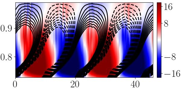
6     V.N. Obridko, V.V. Pipin, D.D. Sokoloff, A.S. Shibalova

                latitude

                                                   Br,[G]

                                                                                                                      [G]
                                                                                     [G]
                                                                                           r/R
                                                            r/R
                                                             c)                             e)
                      a)

                                                   Br,[G]

                                                                                                                     [G]
                                                                                     [G]
                                                                                           r/R
                                                            r/R
                  r/R

                       b)                                    d)                             f)
                                    yr                               yr                                    yr

Figure 5. a) The time-latitude diagrams of the toroidal magnetic field (contours in the range of ±1kG) in the subsurface shear layer,
r=0.9R and the radial magnetic field on the surface (background image); b) the time-radius diagram for the large-scale magnetic field at
the latitude of 30◦ ; c) the time-radius evolution of the axisymmetric mode of the radial magnetic field `1 ; d), e), and f) show the same
for `3 , `5 , and `7 .

                t=32.1yr                                             t=35.5yr

                           t=39yr                                      t=42.4yr

                                         Br, [G]                                                 Br, [G]
Figure 6. Snapshots of the surface magnetic field distributions in a dynamo cycle. The radial magnetic field is shown by color and the
toroidal magnetic field, by contours in the same range of ±20G.

possible. Also, we do not try to resolve the real spatial scale of           Figure 6 illustrates the snapshots of the surface magnetic
the sunspots active regions. This is rather expensive compu-              field distributions during a dynamo cycle starting from the
tationally. The 2D analog of the model was recently discussed             minimum of the magnetic activity. The model shows solar-like
by Pipin (2021). The model should be considered as a numer-               patterns of the magnetic field distribution during the grow-
ical experiment. It does not pretend to explain the emergence             ing and maximum phases of the magnetic activity. Comparing
of the solar active regions. The further details concerning the           these results with Vidotto et al. (2018), we find that the mag-
nonaxisymmetric dynamo model are given in the Appendix                    netic field distribution patterns agree with the low-resolution
A.                                                                        patterns of the magnetic activity found in observations.
   Figure 5 shows the time-latitude and the time-radius di-                  The magnitude of the nonaxisymmetric magnetic field in
agrams of the large-scale magnetic field evolution, as well               these snapshots is rather small compared to the sunspot
the time-radius evolution of the first four odd axisymmetric              magnetic field. This is due to our model restrictions on the
spherical harmonics in the nonaxisymmetric dynamo model.                  strength and size of the bipolar region. However, the ampli-
The results for the axisymmetric modes `1−7 are qualitatively             tude of the generated radial magnetic field flux agrees with
similar to the results of the axisymmetric model. However,                observations to the order of magnitude. The total flux of the
the time-radius evolution of the radial magnetic field at the             radial magnetic field in the model is about 6 1023 Mx (see
latitude of 30◦ shows the difference. The radial magnetic field           Figure7a). This is lower than the value reported by Schrijver
generated in the subsurface shear layer drifts downward from              & Harvey (1994) (1024 Mx) and higher than the flux obtained
the surface and has the opposite sign to the magnetic field               in the WSO low-resolution observations. The total magnetic
propagating from the depth of the convection zone. The pole-              flux of the radial magnetic field in the model evolves in phase
ward surges in the time-latitude diagram of the large-scale ra-           with the toroidal magnetic field activity in the subsurface
dial magnetic field are due to the formation of bipolar regions.          shear layer. The magnetic flux of the axisymmetric magnetic
There are similar radial surges in the time-radius diagrams.              field is shifted by π/2 relative to the evolution of the axisym-

MNRAS 000, 000–000 (0000)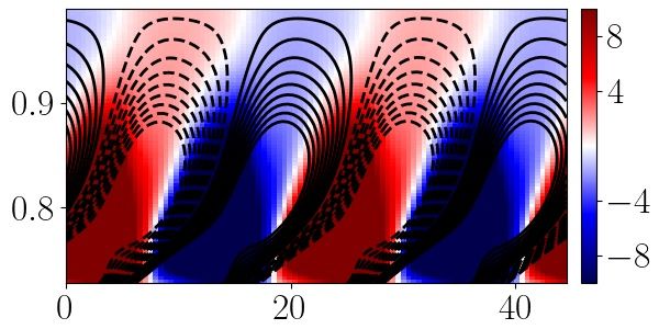
Solar large-scale magnetic field and cycle patterns in solar dynamo                  7
[Mx]

       a)

                                                                            a)

       b)

Figure 7. a) FS is the total unsigned flux of the radial magnetic
             (ax)
field and FS      is the same for the contribution of the axisym-
metric magnetic field; b) Pnx is the parameter characterizing the
nonaxisymmetry of the surface radial magnetic field, PBr is the
equatorial parity parameter of the surface radial magnetic field,
and PBrf is the same for the nonaxisymmetric radial magnetic field.

metric toroidal magnetic field. Using decomposition of the                  b)
radial magnetic field into the partial dynamo modes:
                          X (m)                                           Figure 8. The same as Figures 4 for the nonaxisymmetric dynamo
                  hBr i =     Br (µ) eimφ ,                               model.

where the case m = 0 corresponds to the axisymmetric mag-
netic field, we compute the degree of nonaxisymmetry of the                  The model shows substantial variations in the parity pa-
magnetic field:                                                           rameters of the axisymmetric, PBr , and non-axisymmetric,
                                                   (m)                    PBr
                                                                            f , radial magnetic field. In the model, the emergence of
                                                 Ẽr
                               Pnx      =          (m)
                                                         ,          (7)   the bipolar region is random in longitude and hemisphere.
                                                 Er                       This induces the hemispheric asymmetry of the sources of
where                                                                     the radial magnetic field. In our model the parity varies from
                                1 X
                                    Z                                     -1 to the values which are slightly above zero level. The zero
                    Ẽr(m) =          Br(m) Br(m)∗ dµ,              (8)   parity means a strong hemispheric asymmetry of the mag-
                               8π
                                  m≥1                                     netic activity. The obtained parity variations agree with the
            (m)                                                           results of observations shown in Fig.1. The results of our
and Er is the total energy of the radial component of the
                                                                          model are qualitatively similar to those demonstrated by the
magnetic field. Using decomposition of the radial magnetic
                                                                          3D Babcock-Leighton type model of Hazra & Nandy (2019).
field into spherical harmonics, we compute the two parity
                                                                          When comparing the results of the two dynamo models, we
indices:
                                                                          have to take into account the difference in the parity parame-
                      P (`even )2 P (`odd )2
                        Br       − Br                                     ter definitions. Our definition of the parity parameter reflects
              PBr =                          ,         (9)
                             P (`)2
                                 Br                                       the difference between the energy of a symmetric and anti-
                                                                          symmetric magnetic field about the equator (see, Branden-
where summation is done for all modes, and a similar one for              burg et al. 1989; Knobloch et al. 1998). Also, our model covers
the nonaxisymmetric modes:                                                the period of only a few magnetic cycles. The dynamo simu-
                                                                          lations of (Moss et al. 2008; Weiss & Tobias 2016; Kitchati-
                         Pm>0
                                Br
                                     (`even )2   (`
                                          − m>0 Br odd
                                            P          )2                 nov et al. 2018; Hazra & Nandy 2019) display much stronger
                  PBr
                   f =                 Pm>0 (`)2          .        (10)   long-term parity variations. The above cited papers show that
                                           Br
                                                                          these variations can result both from fluctuations of the α ef-
Figure 7b shows the evolution of these parameters in the                  fect and from hemispheric randomness in the formation of
nonaxisymmetric dynamo model. In general we see a qual-                   a bipolar region. Such long-term variations are beyond the
itative agreement of our results with the observation data                scope of this paper.
represented in Figure 2. In this phase of the magnetic cy-                   Figure 8 shows the integral wavelets of the low axisymmet-
cle, the parameter Pnx is minimum, i.e., the energy of the                ric modes and their cross-correlations with the `5 mode for
nonaxisymmetric magnetic field reaches the lowest value.                  the nonaxisymmetric dynamo model. The obtained results

                                                                                                             MNRAS 000, 000–000 (0000)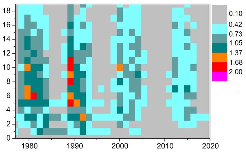
8          V.N. Obridko, V.V. Pipin, D.D. Sokoloff, A.S. Shibalova

Table 3.     Phase shifts (years) for the run C2 (see,             sources and by nonlinearities involved in the dynamo pro-
Pipin&Kosovichev, 2020) and the nonaxisymmetric dynamo model       cesses.
(NXDY).                                                               In our model, the surface poloidal magnetic field originates
                                                                   from two sources: the poloidal magnetic field, which propa-
              C2      Period   NXDY, Period                        gates with the dynamo wave from the depth of the convection
              -2.               -2.5                               zone, and the solar active regions that, in turn, are associated
    g10                11.3             10.8
             0.17π             0.23π                               with the dynamo driven toroidal magnetic field in the sub-
                                                                   surface shear layer. This is similar to studies of Passos et al.
             -3.45              -3.9
    g30                10.7             11.3                       (2014), Hazra et al. (2014) and Hazra & Nandy (2019). Their
             0.3π              0.37π
                                                                   models employed the Babcock-Leighton type scenario as the
    g50                11.3      0      10.6                       main dynamo process. The need for a weak background dis-
                                                                   tributed dynamo was justified by the temporal parameters
              1.1               1.81
    g70                11.3             10.7                       of the magnetic activity during the Maunder minimum. The
             0.08π             0.18π
                                                                   relative contribution of both sources is not known in advance
              -1.8              -2.1                               and may be specific for each harmonic. The polar magnetic
    Bpol               11.3             10.8
             0.15π             0.21π                               field seems to be most directly connected with the propa-
              3.95               3.1                               gation of the poloidal magnetic field from the domain of the
    Bφ                 10.6             10.8                       solar dynamo action, just because sunspots and active regions
             -0.35π            -0.29π
                                                                   are located at middle solar latitudes.
                                                                      Another interesting observational phenomenon is the ex-
agree with observations illustrated in Figures 4, except for
                                                                   citation of even modes during the maximum phases of the
the phase shift between the modes `5 and `7 . We find that
                                                                   sunspot activity. This results in variation of the parity index
the effect of nonaxisymmetric magnetic fields brings the cor-
                                                                   PBr around zero (see, Figs.1 and 4). This effect is readily
relation between `5 and the strength of the toroidal magnetic
                                                                   connected with the hemispheric asymmetry of the magnetic
field in agreement with observations.
                                                                   activity. It was extensively discussed by DeRosa et al. (2012)
   The Table 3 provides the phase shifts and the dynamo pe-        and Hazra & Nandy (2019) as the source of long-term vari-
riods of the low axisymmetric modes and the integral param-        ations of the magnetic activity. The models of the Babcock-
eters for our dynamo models.                                       Leighton type show that the stochastic emergence of active
                                                                   regions and the induced stochastic variations of the α-effect
                                                                   can explain both the long-term variations of the solar activity
                                                                   and variations in the hemispheric asymmetry of the activity
6 CONCLUSION AND DISCUSSION                                        (Kitchatinov et al. 2018; Bhowmik & Nandy 2018; Nepom-
Let us summarize the main results of our study. Observations       nyashchikh et al. 2019; Hazra & Nandy 2019). Note, that
show the difference in the oscillation frequencies of the large-   beating between the modes, when they have close but differ-
scale magnetic field spherical harmonics. Also, the low ` ax-      ent periods, is often considered as a source of long-term vari-
isymmetric harmonics display a phase shift relative to each        ation of the solar magnetic activity (Brandenburg et al. 1989;
other and relative to the proxy of the polar magnetic field        Sokoloff & Nesme-Ribes 1994; Knobloch et al. 1998; Feynman
strength and the sunspot number index. Earlier this phase          & Ruzmaikin 2014; Weiss & Tobias 2016; Beer et al. 2018).
shift was discussed by Stenflo (1994). Our findings show a a       The random fluctuations of the dynamo governing parame-
factor twice less shift’s magnitudes. This is likely due to the    ters are usually considered as the main drivers of long-term
difference of the time-series interval and the method of anal-     variations of the sunspot activity (see the above cited papers).
ysis. Indeed, the time-series in Fig3 seems to show a twice        The long-term parity variations cause a phase-shift between
larger shifts which is in agreement with results of Stenflo        the magnetic activity in the North and South solar hemi-
(1994) for period before 1990 year. Therefore the times shifts     spheres (e.g., Shibalova et al. 2016; Beer et al. 2018; Hazra
between the ` harmonics are not constant.                          & Nandy 2019). These long-term variations are accompanied
   Combining results of this and previous study of DeRosa          by variations in the magnitude and period of a sunspot cycle
et al. (2012) we see that the phase shift between the modes        (Hathaway 2015). It is likely, that stochastic fluctuations of
depends on the spatial sources of the dynamo processes. For        the dynamo parameters can drive the phase shifts and fre-
example, the dynamo model by DeRosa et al. (2012) shows            quencies of the individual ` harmonics as well.
nearly synchronous oscillations with the zero phase shift. Our       Acknowledgements
models are based on the distributed dynamo, and they show
                                                                      The authors are grateful to the WSO teams for a free ac-
different phases for the low ` modes. Both observations and
                                                                   cess to their data. The work was supported by RFBR grants
the dynamo model show an exceptional role of the axisym-
                                                                   No. 20-02-00150,19-52-53045. DS was supported by BASIS
metric `5 mode. Its origin seems to be readily connected with
                                                                   found number 18-1-1-77-3. VVP thanks the financial support
the formation and evolution of sunspots on the solar surface.
                                                                   of the Ministry of Science and Higher Education of the Rus-
The fluctuating nature of this process can result in a disper-
                                                                   sian Federation (Subsidy No.075-GZ/C3569/278).
sion of the dynamo periods. We find that the cycle periods
and the phase shifts of the low ` modes are different in the          Data Availability Statements. The data underlying this ar-
axisymmetric and nonaxisymmetric models. Thus, the asyn-           ticle are available at SIDC (2019). The data of the nonaxisym-
chronous and shifted cycles of the mode can be accounted           metric dynamo model are available at zenodo, Pipin,V.V.
for both by the specific spatial distribution of the dynamo        (2021).

MNRAS 000, 000–000 (0000)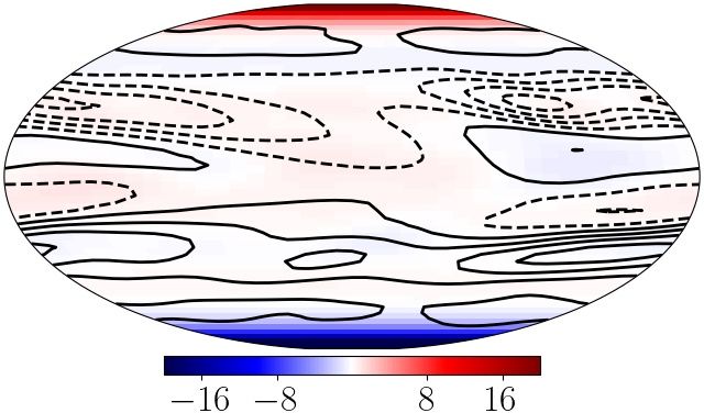
Solar large-scale magnetic field and cycle patterns in solar dynamo                              9
REFERENCES                                                           Obridko V. N., Sokoloff D. D., Shelting B. D., Shibalova A. S.,
                                                                         Livshits I. M., 2020, MNRAS, 492, 5582
Acheson D. J., Gibbons M. P., 1978, Journal of Fluid Mechanics,
                                                                     Parker E. N., 1979, Cosmical magnetic fields: Their origin and their
    85, 743                                                              activity. Oxford: Clarendon Press
Altrock R. C., 1997, Sol. Phys., 170, 411                            Passos D., Nandy D., Hazra S., Lopes I., 2014, A&A, 563, A18
Beer J., Tobias S. M., Weiss N. O., 2018, MNRAS, 473, 1596           Pipin V. V., 2021, Journal of Plasma Physics, 87, 775870101
Benevolenskaya E. E., 2004, A&A, 428, L5                             Pipin V. V., Kosovichev A. G., 2015, The Astrophysical Journal,
Bhowmik P., Nandy D., 2018, Nature Communications, 9, 5209               813, 134
Bigazzi A., Ruzmaikin A., 2004, ApJ, 604, 944                        Pipin V. V., Kosovichev A. G., 2018, ApJ, 867, 145
Brandenburg A., 2005, Astrophys. J., 625, 539                        Pipin V. V., Kosovichev A. G., 2019, ApJ, 887, 215
Brandenburg A., 2018, Journal of Plasma Physics, 84, 735840404       Pipin V. V., Kosovichev A. G., 2020, ApJ, 900, 26
Brandenburg A., Krause F., Meinel R., Moss D., Tuominen I.,          Pipin,V.V. 2021, Data of nonaxisymmetric dynamo model,
    1989, A&A, 213, 411                                                  doi:10.5281/zenodo.4662308
Cameron R. H., Schüssler M., 2017, A&A, 599, A52                     SIDC 2019, Monthly Report on the International Sunspot Number,
Charbonneau P., 2020, Living Reviews in Solar Physics, 2, 2              online catalogue, http://www.sidc.be/sunspot-data/
Dasi-Espuig M., Solanki S. K., Krivova N. A., Cameron R., Peñuela    Scherrer P. H., Wilcox J. M., Svalgaard L., Duvall T. L. J., Dittmer
    T., 2010, A&A, 518, A7                                               P. H., Gustafson E. K., 1977, Sol. Phys., 54, 353
Davies C. R., Hughes D. W., 2011, ApJ, 727, 112                      Schrijver C. J., Harvey K. L., 1994, Sol. Phys., 150, 1
DeRosa M. L., Brun A. S., Hoeksema J. T., 2012, ApJ, 757, 96         Shibalova A. S., Obridko V. N., Sokoloff D. D., 2016, Astronomy
Feynman J., Ruzmaikin A., 2014, Journal of Geophysical Research          Reports, 60, 949
    (Space Physics), 119, 6027                                       Sokoloff D., Nesme-Ribes E., 1994, A&A, 288, 293
Gilman P. A., 1970, ApJ, 162, 1019                                   Stein R. F., Nordlund Å., 2012, ApJ, 753, L13
Gilman P. A., 2018, ApJ, 867, 45                                     Stejko A. M., Kosovichev A. G., Pipin V. V., 2021, arXiv e-prints,
Gizon L., Cameron R. H., Pourabdian M., Liang Z.-C., Fournier            p. arXiv:2101.01220
    D., Birch A. C., Hanson C. S., 2020, Science, 368, 1469          Stenflo J. O., 1994, in Rutten R. J., Schrijver C. J., eds, NATO Ad-
Gokhale M. H., Javaraiah J., 1992, Sol. Phys., 138, 399                  vanced Study Institute (ASI) Series C Vol. 433, Solar Surface
Gokhale M. H., Javaraiah J., Kutty K. N., Varghese B. A., 1992,          Magnetism. p. 365
    Sol. Phys., 138, 35                                              Stenflo J. O., Kosovichev A. G., 2012, ApJ, 745, 129
Hathaway D. H., 2015, Living Reviews in Solar Physics, 12, 4         Stenflo J. O., Vogel M., 1986, Nature, 319, 285
Hazra S., Nandy D., 2019, MNRAS, 489, 4329                           Stenflo J. O., Weisenhorn A. L., 1987, Sol. Phys., 108, 205
Hazra S., Passos D., Nandy D., 2014, ApJ, 789, 5                     Svalgaard L., Duvall T. L. J., Scherrer P. H., 1978, Sol. Phys., 58,
Hoeksema J. T., 1984, PhD thesis, Stanford Univ., CA.                    225
Hoeksema J. T., 1991, Advances in Space Research, 11, 15             Usoskin I. G., 2017, Living Reviews in Solar Physics, 14, 3
Hoeksema J. T., 1995, Space Sci. Rev., 72, 137                       Vidotto A. A., Lehmann L. T., Jardine M., Pevtsov A. A., 2018,
Howe R., Larson T. P., Schou J., Hill F., Komm R., Christensen-          MNRAS, 480, 477
    Dalsgaard J., Thompson M. J., 2011, Journal of Physics Con-      Wang Y. M., Nash A. G., Sheeley N. R. J., 1989, ApJ, 347, 529
    ference Series, 271, 012061                                      Warnecke J., Rheinhardt M., Tuomisto S., Käpylä P. J., Käpylä
Käpylä M. J., Käpylä P. J., Olspert N., Brandenburg A., Warnecke         M. J., Brandenburg A., 2018, A&A, 609, A51
    J., Karak B. B., Pelt J., 2016, A&A, 589, A56                    Weiss N. O., Tobias S. M., 2016, MNRAS, 456, 2654
Kitchatinov L. L., Pipin V. V., 1993, A&A, 274, 647
Kitchatinov L. L., Mordvinov A. V., Nepomnyashchikh A. A.,
    2018, A&A, 615, A38
Kitiashvili I. N., Kosovichev A. G., Wray A. A., Mansour N. N.,
                                                                     7 APPENDIX
    2010, ApJ, 719, 307                                              A. Nonaxisymmetric dynamo model
Knaack R., Stenflo J. O., 2005, A&A, 438, 349
Knobloch E., Tobias S. M., Weiss N. O., 1998, MNRAS, 297, 1123       Evolution of the large-scale magnetic field in perfectly con-
Kosovichev A. G., Pipin V. V., Zhao J., 2013, in Shibahashi H.,      ductive media is described by the mean-field induction equa-
    Lynas-Gray A. E., eds, Astronomical Society of the Pacific       tion Krause & Rädler (1980):
    Conference Series Vol. 479, Progress in Physics of the Sun
    and Stars: A New Era in Helio- and Asteroseismology. p. 395                      ∂t hBi = ∇ × (E+ hUi × hBi) ,                  (11)
    (arXiv:1402.1901)
                                                                     where E = hu × bi is the mean electromotive force; u and
Krause F., Rädler K.-H., 1980, Mean-Field Magnetohydrodynam-
                                                                     b are the turbulent fluctuating velocity and magnetic field,
    ics and Dynamo Theory. Berlin: Akademie-Verlag
Kumar R., Jouve L., Nandy D., 2019, A&A, 623, A54
                                                                     respectively; and hUi and hBi are the mean velocity and
Levine R. H., 1977, ApJ, 218, 291                                    magnetic field. It is convenient to represent the vector hBi
Losada I. R., Warnecke J., Glogowski K., Roth M., Bran-              in terms of the axisymmetric and non-axisymmetric compo-
    denburg A., Kleeorin N., Rogachevskii I., 2017, in Var-          nents as follows:
    gas Domínguez S., Kosovichev A. G., Antolin P., Harra L.,
                                                                                  hBi    =   B + B̃ ,                               (12)
    eds, IAU Symposium Vol. 327, Fine Structure and Dynam-
    ics of the Solar Atmosphere. pp 46–59 (arXiv:1704.04062),                       B    =   φ̂B + ∇ × Aφ̂ ,                        (13)
    doi:10.1017/S1743921317004306
Moss D., Sokoloff D., Usoskin I., Tutubalin V., 2008, Solar Phys.,                  B̃   =   ∇ × (rT ) + ∇ × ∇ × (rS) ,             (14)
    250, 221
Nandy D., Choudhuri A. R., 2001, ApJ, 551, 576                       where B and B̃ are the axisymmetric and nonaxisymmetric
Nepomnyashchikh A., Mandal S., Banerjee D., Kitchatinov L.,          components, A, B, T and S are the scalar functions repre-
    2019, A&A, 625, A37                                              senting the field components, φ̂ is the azimuthal unit vector,
Obridko V. N., Yermakov F. A., 1989, Astronomicheskij Tsirkul-       r is the radius vector, r is the radial distance, and θ is the
    yar, 1539, 24                                                    polar angle. Krause & Rädler (1980) showed that the only

                                                                                                          MNRAS 000, 000–000 (0000)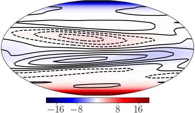
10 V.N. Obridko, V.V. Pipin, D.D. Sokoloff, A.S. Shibalova
1.00
449 1013 a) b)
0.75 431
413 1012
396
CM2/S
0.50
378 1011 νT
360 ηT+η||
0.25 10 η||
10
342 I
0.0 324 b)
a) 0.0 r/ R 0.5 1.0 0.7 0.8 r/ R 0.9
4
2 αφφ Figure 10. a) Snapshot of the axisymmetric magnetic field distri-
M/ S
αrr bution in the convection zone in the growing phase of the magnetic
αθθ M/ S cycle, color shows the toroidal magnetic field strength and contours
0
αrθ show streamlines of the poloidal magnetic field (solid lines - clock-
wise direction); b) color image shows the instability parameter I
−2 (see, Eq19), contour line shows the toroidal magnetic field strength
c) 0.7 0.8 r/ R 0.9 d)
of 500G.
Figure 9. a) The basic angular velocity profile and the stream- & Kosovichev (2018) we put
lines of the meridional circulation with the maximum circulation
velocity of 13 m/s on the surface at the latitude of 45◦ ; b) radial αM LT u0 2
Vβ = − β K (β) (1 + ξβ (t, r, φ, θ)) , (18)
profiles of the total, ηT + η|| , and the rotationally induced part, γ
η|| , of the eddy magnetic diffusivity and the eddy viscosity profile;
c) radial profiles of the α-effect tensor at the latitude of 45◦ ; and where αMLT = 1.9 is the mixing-length theory parameter,
d) the effective drift velocity due to the meridional circulation and γ is the adiabatic law constant, Λ(ρ) = ∇ log ρ; functions
(a)
the turbulent pumping effect. f1,3 and K (β) are given in Kitchatinov & Pipin (1993). The
parameter ξβ determines the magnetic buoyancy velocity per-
turbations. The position of the unstable layer was computed
gauge transformation for potentials T and S is a sum with following the consideration of Parker (1979). It is assumed
the arbitrary r-dependent function. To fix this arbitrariness that the large-scale toroidal magnetic field becomes unstable
they suggested the following normalization: when its strength decreases outward faster than the mean
Z 2π Z 1 Z 2π Z 1
density does. In particular, we compute the parameter
Sdµdφ = T dµdφ = 0. (15)
0 −1 0 −1 ∂ B
I = −r log , (19)
We are using the same formulation for the mean electro- ∂r ρ
motive force as in the recent paper by Pipin & Kosovichev
(2019): where B is the strength of the toroidal magnetic field and
ρ is the density profile. For the unstable part of the toroidal
(A) (P )
Ei = Ei + Ei , (16) magnetic field I > 0. Note, that the magnetic buoyancy insta-
(A)
Ei = (αij + γij ) hBij − ηijk ∇j hBik , bility can be affected by the stellar turbulence and the global
rotation (Gilman 1970; Acheson & Gibbons 1978; Davies &
(P )
Ei = αβ δiφ hBiφ − Vβ (r̂ × hBi)i , (17) Hughes 2011; Gilman 2018). We do not consider these effects
where we divide the expression of the mean electromotive in our simple model. Figure 10 shows snapshots of the mag-
force into the “standard” and phenomenological parts. The netic field and the instability parameter distributions during
standard part of Ei
(A)
contains contributions of the α-effect the growing phase of the magnetic cycle. We see, that in our
tensor, αij , the antisymmetric tensor γij accounts for the tur- model the unstable layers of the toroidal magnetic field are
bulent pumping of the large-scale magnetic fields due to the connected with the bottom of the convection zone and the
effects of the global rotation and density stratification, and subsurface shear layer.
ηijk is the eddy magnetic diffusivity tensor. This corresponds The ξβ perturbations are initiated within the upper layer
to the expression of the mean electromotive force employed in I > 0; initiations are random in time. They go as a Gaus-
the mean-field dynamo models of Pipin & Kosovichev (2019, sian sequence with the mean cadence equal to a month. The
(A) Gaussian sequences of ξβ in the north and south hemispheres
2020). The further details concerning Ei can be found in
are independent. Similar to Pipin & Kosovichev (2018), we
the above-cited papers. Figure 9 shows the large-scale flow
define ξβ as follows,
distribution, the radial profiles of the eddy magnetic diffu-
sivity, the α-effect, and the effective drift velocity due to the φ − φ0 θ − θm
ξβ = Cβψexp −mβ sin2 +sin2 , (20)
meridional circulation and the turbulent pumping effect. 2 2
The phenomenological part of the mean-electromotive force
where ψ is a kink-type function in radius and time,
is introduced to account for the surface effects of the emerg-
2
ing magnetic active region on the large-scale dynamo. It is
τ0 − t
assumed that the toroidal magnetic field in the upper part 1 −
ψ = 1−erf (50 (r − rm ))2 e
2τ0 , t < δt (21)
of the convection zone can be buoyantly unstable and forms 2
magnetic bipolar regions on the solar surface. Following Pipin = 0, t > δt ,
MNRAS 000, 000–000 (0000)Solar large-scale magnetic field and cycle patterns in solar dynamo 11
metric modes of the magnetic field. For example, we have
α hBiφ = αB + α̃B̃φ and the same is true for other sim-
ilar terms. Note that the second part of this formula, the
term α̃B̃φ , as well as the terms like αβ hBiφ and similar ones
that are related to the magnetic buoyancy, are usually ig-
nored in standard mean-field dynamo models. In general, we
can see some similarity between the effect due to α̃B̃φ and
the non-local α-effect employed in the flux-transport mod-
els (Cameron & Schüssler 2017). In our approach, we explic-
a)
YR itly take into account the dynamics of the nonaxisymmetric
magnetic field and its averaged effect on the evolution of the
large-scale magnetic field. To get the evolution equation for
the nonaxisymmetric potential S we substitute Eq(14) into
Eq(11) and, then, calculate the scalar product with vector
r̂. Similarly, the equation for T is obtained by taking curl of
Eq(11) and, then, the scalar product with vector r̂. The pro-
cedure was described in detail by Krause & Rädler (1980).
See also Bigazzi & Ruzmaikin (2004) and Pipin & Kosovichev
b)
(2015). The equations for the potentials T and S are
∂t ∆Ω S = ∆Ω U (U ) + ∆Ω U (EA) + ∆Ω U (EP ) , (25)
Figure 11. The same as Fig.8 for axisymmetric dynamo model. ∂t ∆Ω T = ∆Ω V (U )
+ ∆Ω V (EA)
+ ∆Ω V (EP)
, (26)
where we introduce new notations
the longitude φ0 is random; θm and rm are the latitude and
radius of the extreme points of the toroidal magnetic field in ∆Ω V (U ) = −r̂ · ∇ × ∇ × U × B̃ , (27)
the upper part of the convection zone, where the instability ∆Ω V (E) = −r̂ · ∇ × ∇ × E, (28)
parameter I > 0. We restrict the active phase time, δt, of the
(U )
bipolar region evolution to one week. The emergence interval ∆Ω U = −r̂ · ∇ × U × B̃ , (29)
of the bipolar region is controlled by the parameter τ0 . In
our simulations we put it to 3 days, which corresponds to the ∆Ω U (E) = −r̂ · ∇ × E. (30)
observation results (see, Stenflo & Kosovichev (2012)). The (U )
We do not show details of ∆Ω U, V as well as the standard
parameter Cβ = 200 is chosen in such a way that the un- parts of the ∆Ω U, V (E) terms. Their derivation is described
stable part of the axisymmetric magnetic field could emerge in detail in the above-cited papers. For the nonaxisymmetric
on the surface after time τ0 starting from the level r=0.9R, parts related to the magnetic buoyancy and αβ the effect
which corresponds to the mean level of the magnetic buoy- reads as follows
ancy instability of the large-scale toroidal magnetic field in 1 ∂ ∂
the upper part of the convection zone. In this model we do ∆Ω V (EP ) = − (r hBθ i Vβ )
r sin θ ∂φ ∂r
not intend to reproduce the spatial parameters of the sunspot
bipolar regions. For the sake of numerical efficiency we put ∂ sin θ ∂
− (r hBφ i Vβ ) (31)
mβ = 20, which results in large-scale bipolar regions, (see, ∂µ r ∂r
Figure 6). The α-effect will be given as follows 1 ∂ 1 ∂
− r αβ hBφ i ,
αβ = 0.3 cos θVβ , (22) r ∂r sin θ ∂φ
where Vβ is determined by Eq(18), and the coefficient 0.3 was 1 ∂ ∂
chosen from numerical experiments. With our representation ∆Ω U (EP ) = − (hBφ i Vβ ) + (sin θ hBθ i Vβ )
sin θ ∂φ ∂µ
of the mean electromotive force in the form of Eq(16), the ∂
full version of the dynamo equations for the axisymmetric + αβ hBφ i .
∂µ
magnetic field reads as follows,
(A) Vβ ∂ (rA)
∂t A = Eφ + αβ hBφ i + + Vβ B̃θ , (23) B. Results of axisymmetric dynamo model
r ∂r
sin θ ∂ (r sin θA, Ω) 1 ∂ 2
Here we reproduce some results of the run C2 from Pipin
∂t B = − r Vβ B + Vβ B̃φ
r ∂ (r, µ) r ∂r & Kosovichev (2020). See the above-cited paper for details
(A) of the model. Figure 11a shows variations in the first four
(1 − µ ) ∂Er(A)
p
2
1 ∂rEθ
+ + , (24) odd axisymmetric spherical harmonics on the surface, as well
r ∂r r ∂µ
as the evolution of the mean polar magnetic field and the
where, the contribution of E (A) stands for the standard part mean density of the toroidal field in the subsurface layer,
of the mean-electromotive force, its details are omitted. For r = 0.9 − 0.99R. The parameter Bφ is considered a proxy
the sake of brevity, the αβ -effect and magnetic buoyancy for the sunspot number. The integral wavelets of the low ax-
terms are written explicitly via the magnetic field compo- isymmetric modes and their cross-correlations with `5 mode
nents. Besides, these contributions bear the effect of the non- are shown in Figure11b. The toroidal magnetic field and the
linear coupling between the axisymmetric and nonaxisym- `3 harmonic show periods of about 10.6 years. The polar
MNRAS 000, 000–000 (0000)12 V.N. Obridko, V.V. Pipin, D.D. Sokoloff, A.S. Shibalova
Br,[G]
latitude
[G]
[G]
r/R
c) e)
a)
[G]
Br,[G]
[G]
r/R
r/R
b) d) f)
yr yr yr
Figure 12. The same as Fig.5 for axisymmetric dynamo model.
magnetic field, as well as the `1,5,7 axisymmetric harmonics
show a period of about 11.3 years. The axisymmetric modes
show an auxiliary peak around 5 years. In the axisymmetric
model, the correlation of the mode `5 with other axisymmet-
ric modes, as well as with the integral parameters Bpol and
the sunspot proxy Bφ agrees qualitatively with observations
(see, Figure11b). The correlation between `5 and `7 shows
the largest difference compared to the observation results.
The time-latitude and time-radius diagrams of the large-scale
magnetic field evolution, as well as the time-radius evolution
of the first four odd axisymmetric spherical harmonics are
shown in Figure 12. The butterfly diagram of the model qual-
itatively agrees with observations. At the latitude of 30◦ , the
diagram of the time-radius evolution of the toroidal and ra-
dial magnetic field shows a drift of the magnetic field activity
toward the surface. The duration of the drift is about half a
magnetic cycle. It is interesting to note that the axisymmet-
ric harmonics `1 and `7 follow the same direction of the drift.
The `3 harmonic shows a steady wave with two maxima: one
near the bottom and the other at the top of the convection
zone. The `5 harmonic shows a similar tendency. However its
maximum at the top of the convection zone is less pronounced
than for the `3 . In the upper part of the convection zone,
`5 displays an inward drift. Therefore, the model evolution
of the radial magnetic field of `3 and `5 harmonics can be
connected with the toroidal magnetic field in the subsurface
shear layer. Naturally, the `5 maxima at the surface corre-
spond to the maxima of the toroidal magnetic field butterfly
diagrams.
The above consideration reveals the peculiarities in the evo-
lution of the `3 and `5 axisymmetric harmonics of the radial
magnetic field. The harmonic `3 displays a dynamo period
close to the period of the toroidal magnetic field parameter
Bφ in the subsurface layer. This harmonic is shifted ahead by
about π/2 of the toroidal magnetic field evolution and has its
maximum at the surface. Therefore, the surface evolution of
`3 is determined by generation of the radial magnetic field
from the toroidal magnetic field by means of the α-effect.
While the generation of `3 is connected with the rising branch
of the toroidal magnetic field in the subsurface shear layer,
the near-surface generation of `5 is connected with the decay-
ing Bφ there. Observations show that the periods of `5 and
Bφ are close. This means that there may be an additional
near-surface source of the α-effect that produces `5 . We as-
sume that it can be due to the emerging bipolar regions.
MNRAS 000, 000–000 (0000)You can also read