Comparisons between Mean and Turbulent Parameters of Aircraft-Based and Ship-Based Measurements in the Marine Atmospheric Boundary Layer
←
→
Page content transcription
If your browser does not render page correctly, please read the page content below
atmosphere

Article
Comparisons between Mean and Turbulent Parameters of
Aircraft-Based and Ship-Based Measurements in the Marine
Atmospheric Boundary Layer
Min-Seong Kim 1 , Byung Hyuk Kwon 2, * and Tae-Young Goo 1

                                          1   Convergence Meteorological Research Department Aviation Observation Research Team,
                                              National Institute of Meteorological Sciences, Seogwipo 63568, Jeju-do, Korea;
                                              givemeasong@korea.kr (M.-S.K.); gooty@korea.kr (T.-Y.G.)
                                          2   Department of Environmental Atmospheric Sciences, Pukyong National University,
                                              Busan 48513, Gyeongsangnam-do, Korea
                                          *   Correspondence: bhkwon@pknu.ac.kr

                                          Abstract: The Structure des Echanges Mer-Atmosphère, Propriétés Océaniques/ Recherche Expérimentale
                                          (SEMAPHORE) experiment was conducted over the oceanic Azores current located in the Azores
                                          Basin. The evolution of the marine atmospheric boundary layer (MABL) was studied based on the
                                          evaluation of mean and turbulent data using in situ measurements by a ship and two aircrafts. The
                                          sea surface temperature (SST) field was characterized by a gradient of approximately 1 ◦ C/100 km.
                                          The SST measured by aircraft decreased at a ratio of 0.25 ◦ C/100 m of altitude due to the divergence of
                                the infrared radiation flux from the surface. With the exception of temperature, the mean parameters

                                          measured by the two aircrafts were in good agreement with each other. The sensible heat flux was
Citation: Kim, M.-S.; Kwon, B.H.;         more dispersed than the latent heat flux according to the comparisons between aircraft and aircraft,
Goo, T.-Y. Comparisons between            and aircraft and ship. This study demonstrates the feasibility of using two aircraft to describe the
Mean and Turbulent Parameters of          MABL and surface flux with confidence.
Aircraft-Based and Ship-Based
Measurements in the Marine
                                          Keywords: marine atmospheric boundary layer; sea surface temperature; infrared flux divergence;
Atmospheric Boundary Layer.
                                          heat flux; SEMAPHORE
Atmosphere 2021, 12, 1088. https://
doi.org/10.3390/atmos12091088

Academic Editors: Zhenru Shu,
                                          1. Introduction
Pak-Wai Chan and Yuncheng He
                                                The determination of boundary layer conditions at the air–ocean interface is an impor-
Received: 15 June 2021                    tant issue in atmospheric and oceanic predictive numerical models. The air–sea exchanges
Accepted: 20 August 2021                  of momentum, heat, and water are substantial in atmospheric and oceanic movements
Published: 24 August 2021                 at different scales. Accurate predictions of complex and poorly understood marine en-
                                          vironments require an improved understanding of spatial variability and highly precise
Publisher’s Note: MDPI stays neutral      parameterization of turbulent surface flows [1]. The atmospheric turbulent fluxes of heat,
with regard to jurisdictional claims in   water vapor, and momentum across the air–ocean interface play a substantial role in the
published maps and institutional affil-   development of climate and the weather system. Therefore, they should be an integral part
iations.                                  of numerical weather prediction and climate prediction models. Because this exchange
                                          is primarily at the sub-grid scale, it is parameterized by a surface bulk exchange param-
                                          eterization scheme that is semi-empirical. Abundant intensive observations of turbulent
                                          exchange are required to improve the algorithm, typically by estimating the exchange
Copyright: © 2021 by the authors.         coefficients [2,3].
Licensee MDPI, Basel, Switzerland.              Interactions between the ocean and atmosphere have been experimentally studied
This article is an open access article    from turbulence to synoptic scales for several years. Many of the associated studies fo-
distributed under the terms and           cused on the examination of physical processes in the marine atmospheric boundary
conditions of the Creative Commons        layer (MABL) and on surface turbulent fluxes, for example, the Joint Air–Sea Interaction
Attribution (CC BY) license (https://     (JASIN) [4] and the Genesis of Atlantic Lows Experiment (GALE) [5,6]. The horizontal
creativecommons.org/licenses/by/          variability was experimentally revealed for the first time during JASIN and the Frontal
4.0/).

Atmosphere 2021, 12, 1088. https://doi.org/10.3390/atmos12091088                                      https://www.mdpi.com/journal/atmosphere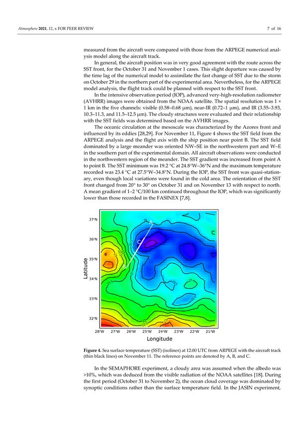
Atmosphere 2021, 12, 1088                                                                                          2 of 15

                            Air–Sea Interaction Experiment (FASINEX) pertaining to the physical processes in atmo-
                            spheric and oceanic boundary layers [7,8]. They were conducted in conditions caused
                            by the presence of a thermal front in the upper ocean. Powell et al. [9] described the
                            transfer of momentum between the atmosphere and the ocean in terms of the vertical
                            variation of wind speed and a drag coefficient that increases with wind speed and sea
                            surface roughness. Persson et al. [10] presented ship-based eddy covariance and inertial
                            dissipation fluxes from the central North Atlantic. Aircraft-based covariance flux ob-
                            servations have been reported for hurricanes [11], during barrier winds and tip jets [12].
                            Haynes et al. [13] examined the Southern Ocean (SO) clouds using multi-satellite prod-
                            ucts and reported that most SO clouds reside in the MABL and, hence, are difficult to
                            accurately detect from space. Owing to a lack of in situ observations, understanding the
                            thermodynamic structure of the MABL in the SO remains a challenge. Truong et al. [14]
                            utilized 2186 high-resolution soundings from four recent field campaigns to construct a
                            climatology profile of the MABL and to examine relationships between the synoptic me-
                            teorology and thermodynamic structure by means of composite analysis of fronts and
                            cyclones in the SO. Williams et al. [15] highlighted that the height of the SO MABL in
                            the Transpose-Atmospheric Model Intercomparison Project simulation was consistently
                            underestimated in comparison to an operational analysis product. However, when com-
                            pared with historical atmospheric soundings over Macquarie Island, the height of the
                            MABL in a reanalysis (European Centre for Medium-Range Weather Forecasts reanalysis
                            (ERA)-Interim) product was underestimated [16,17]. Andreas et al. [3] investigated the
                            dependence of the 10 m drag coefficient in a neutral condition over the sea in the context of
                            the Monin–Obukhov similarity theory by analyzing four different aircraft datasets from
                            11 different experiments.
                                  As aircraft observation is highly convenient in MABL, it is necessary to control the
                            quality and validate the measurement data. The Structure des Echanges Mer-Atmosphère,
                            Propriétés Océaniques/ Recherche Expérimentale (SEMAPHORE) experiment was per-
                            formed from June to November 1993, south of the Azores islands, primarily characterized
                            by a thermal front [18]. An instrumented ship undertook in situ observations and an
                            aircraft undertook remote observations over the sea surface temperature (SST) front [19].
                            The experimental area was situated between 31◦ –38◦ N and 21◦ –28◦ W (500 × 500 km). The
                            SEMAPHORE experiment was performed to improve our knowledge of ocean–atmosphere
                            interactions from the local scale to the mesoscale [19]. Giordani et al. [20] showed the
                            atmospheric response to SST changes based on a numerical model. Kwon et al. [18] and
                            Lambert and Durant [21] dealt with the vertical variation of the turbulence fluxes in PBL af-
                            fected by the SST gradient. Although Lambert and Durant [22] made an aircraft-to-aircraft
                            comparison, turbulence parameters were the main factor and ship observation-based data
                            were not addressed. In the SEMAPHORE experiment performed in this study, the accuracy
                            of surface layer mean and turbulent parameters were evaluated by comparing aircraft data
                            to ship data once the aircraft-to-aircraft comparison was completed.
                                  Absolute calibration of most instruments installed on the aircraft is difficult because
                            the measurements are affected by the airspeed of the sensor. Because there is no absolute
                            reference for in-flight measurements, aircraft-to-aircraft inter-comparisons are the best
                            means to ensure coherence between various platforms [22]. Calibration against ground-
                            based measurements cannot be considered satisfactory owing to the different sampled
                            areas and sampling time for the two platforms. Furthermore, ground-based measurements
                            generally cannot be used over the open ocean. Air-to-air cross-comparison experiments
                            have been conducted during several campaigns; however, the results of applying a cali-
                            bration process compared to in situ ship observations are elusive. To study characteristics
                            of the atmospheric surface layer with remotely sensed data from an aircraft, we validated
                            the observation data obtained by two aircraft, which were compared with the ship-based
                            observation. This paper presents the validation of the data by analyzing the references
                            for SST and atmospheric surface measurements. We discuss the experimental site, exper-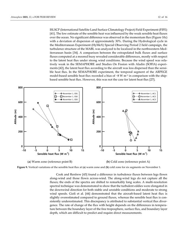
Atmosphere 2021, 12, 1088 3 of 15
imental method, and airborne equipment utilized in the context of the characteristics of
the MABL.
2. Materials and Methods
2.1. Instrumented Aircraft
Two aircraft, the Fokker 27 (ARAT) and the Fairchild Merlin IV (Merlin IV), were
instrumented by the Institut National des Sciences de l’Univers (INSU) and the French
Meteorological Office (FMO), respectively, to investigate the MABL characteristics and
the surface fluxes. The datasets were enhanced with geophysical parameters derived
from meteorological satellites (NOAA, Meteosat, and Defense Meteorological Satellite
Program). This study was completed with the cooperation of the Centre de Recherches
Atmosphériques, one of the SEMAPHORE experiment organizers, eliminating the limita-
tion of data availability (the data of the SEMAPHORE are not currently publicly available).
Both the aircrafts measured atmospheric turbulence and radiation with different sen-
sors. ARAT was installed with a 5 m long nose boom with fast response sensors. A Rose-
mount 858 probe (Rosemount Engineering Co., Eden Prairie, MIN 55344, USA) observed
slide slip and attack angles, along with dynamic and static pressures. An inertial navigation
system (INS) detected the ground velocity, the horizontal geographical position, and the at-
titude angles: roll, pitch, and true heading [23]. On Merlin IV, a radome measured the slide
slip and attack angles, and total pressures [24]. The INS was equipped behind the nose of
ARAT and close to the gravity center of Merlin IV. The temperature was observed by a Rose-
mount 102E2-AL probe (Rosemount Engineering Co., Eden Prairie, MIN 55344, USA) lo-
cated on both aircrafts, and the moisture was observed by a Lyman-α sensor (Buck Research,
Novato, CA 94945-1400, USA) and a dew-point hygrometer [18]. Upward and downward
longwave radiation (4–40 µm band) and shortwave (0.2–2.8 µm band) radiation were mea-
sured using Eppley sensors (The Eppley Laboratory Inc., Newport, RI 02840, USA). The
sea surface brightness temperature was measured by a downward-looking Barnes PRT5
(Barnes Engineering Company, Colorado Springs, CO 80916, USA) thermo-radiometer.
A radio altimeter measured the altitude above the sea level. The SST was corrected to
incorporate the vertical divergence of the longwave radiation from the sea surface to the
flight level of Merlin IV. The incoming radiation, which can be as significant as the surface
emissivity, was excluded for the SST correction.
2.2. Flight Plans
The aircraft observations were performed simultaneously in the same area of the ship.
The wind orientation and the SST front in the MABL was taken into consideration. The
radio-sounding on the ship provided the wind in the experimental zone. During the IOP,
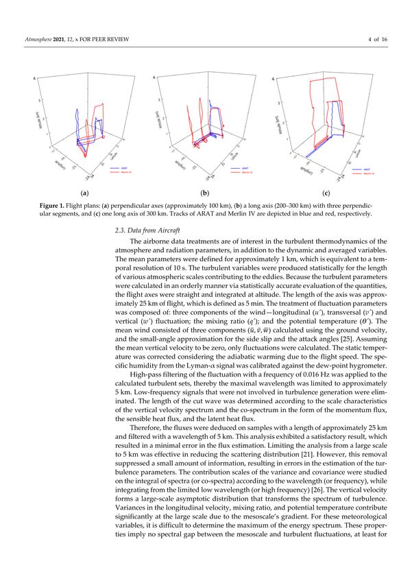
three types of flight plans were used: (i) two long perpendicular tracks of 100 km crossing
the oceanic front in two different regions between 80 m and the top of the mixed layer
or at the bottom of clouds. Three soundings completed the flight plan (Figure 1a). (ii) A
main axis of 200 to 300 km was associated with three perpendicular segments of 30 km at
the middle point and at both ends of the long axis. This flight plan was completed by the
two planes at five different levels with their vertical soundings of up to 2.5 km (Figure 1b).
This flight plan was able to analyze transversal and longitudinal flows in the intermediate
zone. (iii) One flight axis of 300 km was constituted by two or three soundings at the
end of the axis (Figure 1c). This flight plan was adapted for the thermal transitions and
enabled characterization of the atmospheric turbulence along the longest axis. The mean
parameters were averaged, and the turbulent parameters were calculated on segments of
approximately 25 km long. They were named AC1, AC2, and AC3 from point A to C, and
CB1, CB2, CB3, CB4, CB5, CB6, CB7, CB8, and CB9 from point C to B.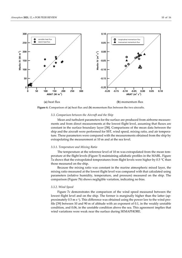
Atmosphere 2021, 12, 1088                                                                                                        4 of 15

      Figure 1. Flight plans: (a) perpendicular axes (approximately 100 km), (b) a long axis (200–300 km) with three perpendicular
      segments, and (c) one long axis of 300 km. Tracks of ARAT and Merlin IV are depicted in blue and red, respectively.

                                  2.3. Data from Aircraft
                                         The airborne data treatments are of interest in the turbulent thermodynamics of the
                                  atmosphere and radiation parameters, in addition to the dynamic and averaged variables.
                                  The mean parameters were defined for approximately 1 km, which is equivalent to a
                                  temporal resolution of 10 s. The turbulent variables were produced statistically for the
                                  length of various atmospheric scales contributing to the eddies. Because the turbulent
                                  parameters were calculated in an orderly manner via statistically accurate evaluation of
                                  the quantities, the flight axes were straight and integrated at altitude. The length of the
                                  axis was approximately 25 km of flight, which is defined as 5 min. The treatment of
                                  fluctuation parameters was composed of: three components of the wind—longitudinal
                                  (u0 ), transversal (v0 ) and vertical (w0 ) fluctuation; the mixing ratio (q0 ); and the potential
                                  temperature (θ 0 ). The mean wind consisted of three components (u, v, w) calculated
                                  using the ground velocity, and the small-angle approximation for the side slip and the
                                  attack angles [25]. Assuming the mean vertical velocity to be zero, only fluctuations were
                                  calculated. The static temperature was corrected considering the adiabatic warming due to
                                  the flight speed. The specific humidity from the Lyman-α signal was calibrated against the
                                  dew-point hygrometer.
                                         High-pass filtering of the fluctuation with a frequency of 0.016 Hz was applied to the
                                  calculated turbulent sets, thereby the maximal wavelength was limited to approximately
                                  5 km. Low-frequency signals that were not involved in turbulence generation were elimi-
                                  nated. The length of the cut wave was determined according to the scale characteristics of
                                  the vertical velocity spectrum and the co-spectrum in the form of the momentum flux, the
                                  sensible heat flux, and the latent heat flux.
                                         Therefore, the fluxes were deduced on samples with a length of approximately 25 km
                                  and filtered with a wavelength of 5 km. This analysis exhibited a satisfactory result, which
                                  resulted in a minimal error in the flux estimation. Limiting the analysis from a large scale
                                  to 5 km was effective in reducing the scattering distribution [21]. However, this removal
                                  suppressed a small amount of information, resulting in errors in the estimation of the tur-
                                  bulence parameters. The contribution scales of the variance and covariance were studied
                                  on the integral of spectra (or co-spectra) according to the wavelength (or frequency), while
                                  integrating from the limited low wavelength (or high frequency) [26]. The vertical velocity
                                  forms a large-scale asymptotic distribution that transforms the spectrum of turbulence.
                                  Variances in the longitudinal velocity, mixing ratio, and potential temperature contribute
                                  significantly at the large scale due to the mesoscale’s gradient. For these meteorological
                                  variables, it is difficult to determine the maximum of the energy spectrum. These properties
                                  imply no spectral gap between the mesoscale and turbulent fluctuations, at least for the hor-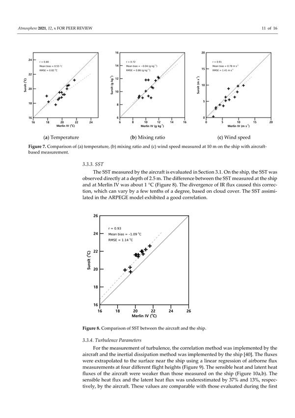
Atmosphere 2021, 12, 1088                                                                                               5 of 15

                            izontal velocities and the scalar variables. Variations in vertical fluxes are more analogous
                            to the variance of the vertical velocity, which is calculated using the correlation method.
                            This means that the flux is controlled by a dynamic mechanism. The turbulent kinetic
                            energy, the vertical momentum flux, and the latent heat were slightly underestimated near
                            the surface and underestimated by 20% at high altitudes [18,19,24].

                            2.4. Infrared (IR) Flux Divergence
                                 A Barnes-PRT5 was used to measure the IR radiation from the sea surface and to pro-
                            duce the brightness temperature along the flight trajectory. Due to the temporal difference
                            of the ARAT sensor, data from Merlin IV was only used for SST correction. The SST was
                            corrected for the divergence of the atmospheric radiation flux between the surface and the
                            flight altitude. In particular, the cloud cover has a significant influence on divergence. The
                            decrease in SST with altitude was restored to take into account the emissivity. If the SST
                            varies with time and space:
                                                                   SST = f ( x, y, (t))                                 (1)
                            The apparent temperature Ta is a function of SST, emissivity, descending IR, and altitude:

                                                           Ta = f SST, ελ, IRde λ , z                              (2)

                            At the surface, the radiation is given by:

                                                         σTa4 = ελσ(SSTλ )4 + (1 − ελ) IRde
                                                                                         λ                                 (3)

                            At the altitude z, the radiation is decreased by the atmospheric absorption:
                                                        h           iz                      h                     iz
                                  σTa4 = ελσ(SSTλ )4 − ∆ ελσ(SSTλ )4 + (1 − ελ) IRde
                                                                                  λ (0) − ∆   ( 1 − ελ ) IR de
                                                                                                            λ (0)          (4)
                                                                           0                                        0

                            If IRde
                                 λ is measured only at altitude z:
                                                                                 h       iz
                                                              IRde       de         de
                                                                λ(z) = IRλ(0) − ∆ IRλ(0)                                   (5)
                                                                                          0
                                                          h            iz                              h       iz
                                   σTa4 = ελσ(SSTλ )4 − ∆ ελσ(SSTλ )4 + (1 − ελ) IRde
                                                                                   λ(z)
                                                                                        + ( 1 − ελ ) ∆   IR de
                                                                                                            λ 0
                                            h                 h     iz iz0                                                 (6)
                                         −∆ (1 − ελ) IRde
                                                        λz + ∆ IRλ
                                                                 de
                                                                         0 0
                            Ignoring the third-order terms:
                                                                       h            iz
                                           σTa4   = ελσ(SSTλ )4      −∆ ελσ(SSTλ )4       +(1 − ελ) IRde
                                                                                                      λ(z)
                                                                                      0                                    (7)
                                             I           II                    III               IV

                            where the left-hand side is the measured radiation at the flight altitude, term II is unknown
                            (ελ and Tλ ), and term III is calculated by a statistical method at different altitudes. In term
                            IV, IRde                                                                             de
                                   λ is measured. When ελ 6 = 0, Ta depends on the vertical variation of IRλ . Figure 2
                            shows the descending IR radiation flux as a function of the SST difference between the
                            ship and the aircraft (SSTship − SSTaircra f t ), which decreases when the IR flux increases.
                            Assuming that the SST and ελ vary little between the two measurements over the same
                            flight trajectory, ελ is calculated and the corrected SST is estimated.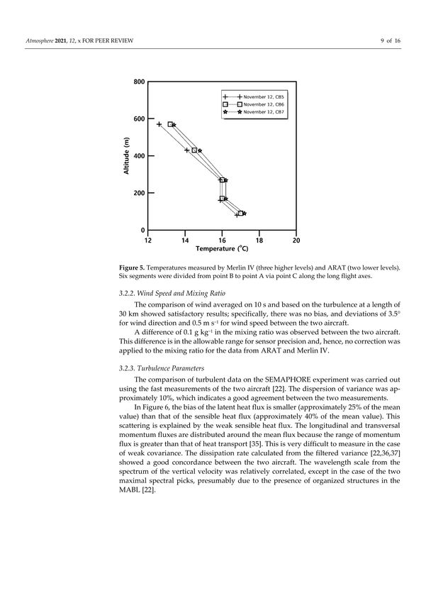
Atmosphere 2021, 12, 1088                                                                                                    6 of 15

                            Figure 2. Descending infrared flux depending on the SST difference (SSTship − SSTaircra f t ).

                                 The SST was corrected on each flight track of approximately 30 km. Figure 3 shows the
                            correction rate of the SST, with altitude plotted against the IR flux divergence. According to
                            the measurement of Merlin IV, the major correction rate was 0.25 ◦ C per 100 m, as shown
                            in the histogram for the different applied days.

                            Figure 3. Percentage of the correction rate with the flight altitude according to Merlin IV.

                            3. Results
                            3.1. SST Field
                                 The SST measured by Merlin IV was, on average, 1 ◦ C lower than that measured by
                            the ship. This is not anomalous, because the measurement system of the ship is different
                            from that of the aircraft; the former measured the water temperature at a depth of 2.5 m,
                            whereas the latter detected the surface brightness temperature incorporating the effects
                            of air–sea interaction. The ship measurements were considered to be a reference for the
                            correction of the aircraft measurements. The SST from buoys and the ship were assimilated
                            in the Action de Recherche Petite Echelle Grande Echelle (ARPEGE) model analysis [27].
                            The temperature front could be easily determined on SST fields for the entire experiment.
                            Thus, the exact direction of the aircraft pattern relative to the iso-SST level was known.
                            In contrast, when the MABL characteristics were analyzed across the SST front, the SST
                            measured along the flight axis was taken into account. In six experiments, the SST values
                            measured from the aircraft were compared with those from the ARPEGE numerical analysis
                            model along the aircraft track.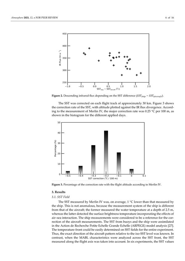
Atmosphere 2021, 12, 1088                                                                                                7 of 15

                                  In general, the aircraft position was in very good agreement with the route across the
                            SST front, for the October 31 and November 1 cases. This slight departure was caused by
                            the time lag of the numerical model to assimilate the fast change of SST due to the storm
                            on October 29 in the northern part of the experimental area. Nevertheless, for the ARPEGE
                            model analysis, the flight track could be planned with respect to the SST front.
                                  In the intensive observation period (IOP), advanced very-high-resolution radiometer
                            (AVHRR) images were obtained from the NOAA satellite. The spatial resolution was
                            1 × 1 km in the five channels: visible (0.58–0.68 µm), near-IR (0.72–1 µm), and IR (3.55–3.93,
                            10.3–11.3, and 11.5–12.5 µm). The cloudy structures were evaluated and their relationship
                            with the SST fields was determined based on the AVHRR images.
                                  The oceanic circulation at the mesoscale was characterized by the Azores front and
                            influenced by its eddies [28,29]. For November 11, Figure 4 shows the SST field from the
                            ARPEGE analysis and the flight axis with the ship position near point B. The SST field
                            dominated by a large meander was oriented NW–SE in the northwestern part and W–E in
                            the southern part of the experimental domain. All aircraft observations were conducted in
                            the northwestern region of the meander. The SST gradient was increased from point A to
                            point B. The SST minimum was 19.2 ◦ C at 24.8◦ W–36◦ N and the maximum temperature
                            recorded was 23.4 ◦ C at 27.5◦ W–34.8◦ N. During the IOP, the SST front was quasi-stationary,
                            even though local variations were found in the cold area. The orientation of the SST front
                            changed from 20◦ to 30◦ on October 31 and on November 13 with respect to north. A mean
                            gradient of 1–2 ◦ C/100 km continued throughout the IOP, which was significantly lower
                            than those recorded in the FASINEX [7,8].

                            Figure 4. Sea surface temperature (SST) (isolines) at 12:00 UTC from ARPEGE with the aircraft track
                            (thin black lines) on November 11. The reference points are denoted by A, B, and C.

                                  In the SEMAPHORE experiment, a cloudy area was assumed when the albedo was >10%,
                            which was deduced from the visible radiation of the NOAA satellites [18]. During the
                            first period (October 31 to November 2), the ocean cloud coverage was dominated by
                            synoptic conditions rather than the surface temperature field. In the JASIN experiment,
                            lower cloud cover was related to SST changes [7,30]. Zelinka and Hartmann [31] reported
                            that clouds were critical factors used to define the budget of regional radiation in the SO
                            region and to transport the energy and moisture from the tropical zone to the Antarctic.
                            However, large differences in cloud amount and properties over the SO were retained
                            in the reanalysis products and in the climate simulations [32,33]. It was difficult for the
Atmosphere 2021, 12, 1088 8 of 15
climate models to produce low-level clouds behind cold fronts and in the cold-air sector of
extratropical cyclones [15]. Brilouet et al. [34] considered that cloud cover/structure height,
or thermodynamic characteristics, are systematically similar. They also found that during
the strong wind periods, the latent and sensible heat flux reached 500 and 300 Wm−2 ,
respectively. Despite intense cold-air outbreaks, the SST variations were weak. In the
SEMAPHORE, based on two AVHRR images per day on different channels, it was found
that no cloud organization was related to the SST field, although pronounced local effects
were observed during the anticyclonic periods.
3.2. Comparison of the Data from the Two Aircrafts
Comparison of data from the two aircraft is an important process, because it deter-
mines the precision of the thermodynamic and dynamic fields acquired under different
experimental conditions. Aircraft are valuable platforms for exploring the ABL; however,
it is difficult to completely standardize measurement devices because measured data are
influenced by the airflow entering the sensor. The standardization of the airborne sensor is
carried out in the laboratory by considering the effects of pressure exerted on the sensors
during the flight [25]. Standardization based on measurements carried out at the surface
cannot be precise. Due to the absence of an absolute reference during the in-flight measure-
ment, comparisons between the two aircraft are the most appropriate means to ensure the
consistency of measurements.
3.2.1. Air Temperature
Air temperature was measured using three probes in each of the two aircraft. The
mean temperature measured by Merlin IV was 0.5 ◦ C higher than that of ARAT between
950 and 900 hPa. There was no defrosted Rosemount probe, resulting in the intermediate
value between the three probes of ARAT. In addition, the difference between the two tem-
perature sensors used as references was approximately 0.7 ◦ C at this altitude [33]. Figure 5
shows vertical profiles of the average temperature measured by the Rosemount probe at a
30 km segment. Adiabatic profiles were found through five levels: the two profiles were
lower as measured by the ARAT and the other three profiles were higher as measured by
Merlin IV. A difference of 0.7 ◦ C was revealed between the air temperatures measured by
the two aircraft. Because the measured static pressures of the two aircraft were coherent,
temperature correction was applied to the potential temperature [21].
Figure 5. Temperatures measured by Merlin IV (three higher levels) and ARAT (two lower levels).
Six segments were divided from point B to point A via point C along the long flight axes.Atmosphere 2021, 12, 1088 9 of 15
3.2.2. Wind Speed and Mixing Ratio
The comparison of wind averaged on 10 s and based on the turbulence at a length of
30 km showed satisfactory results; specifically, there was no bias, and deviations of 3.5◦ for
wind direction and 0.5 m s−1 for wind speed between the two aircraft.
A difference of 0.1 g kg−1 in the mixing ratio was observed between the two aircraft.
This difference is in the allowable range for sensor precision and, hence, no correction was
applied to the mixing ratio for the data from ARAT and Merlin IV.
3.2.3. Turbulence Parameters
The comparison of turbulent data on the SEMAPHORE experiment was carried out
using the fast measurements of the two aircraft [22]. The dispersion of variance was
approximately 10%, which indicates a good agreement between the two measurements.
In Figure 6, the bias of the latent heat flux is smaller (approximately 25% of the mean
value) than that of the sensible heat flux (approximately 40% of the mean value). This
scattering is explained by the weak sensible heat flux. The longitudinal and transversal
momentum fluxes are distributed around the mean flux because the range of momentum
flux is greater than that of heat transport [35]. This is very difficult to measure in the case
of weak covariance. The dissipation rate calculated from the filtered variance [22,36,37]
showed a good concordance between the two aircraft. The wavelength scale from the spec-
trum of the vertical velocity was relatively correlated, except in the case of the two maximal
spectral picks, presumably due to the presence of organized structures in the MABL [22].
Figure 6. Comparison of (a) heat flux and (b) momentum flux between the two aircrafts.
3.3. Comparison between the Aircraft and the Ship
Mean and turbulent parameters for the surface are produced from airborne measure-
ments and from direct measurements at the lowest flight level, assuming that fluxes are
constant in the surface boundary layer [38]. Comparisons of the mean data between the
ship and the aircraft were performed for SST, wind speed, mixing ratio, and air tempera-
ture. These parameters were compared with the measurements obtained from the ship by
extrapolating the measurement at 10 m and at the sea level.
3.3.1. Temperature and Mixing Ratio
The temperature at the reference level of 10 m was extrapolated from the mean
temperature at the flight levels (Figure 5) maintaining adiabatic profiles in the MABL.Atmosphere 2021, 12, 1088 10 of 15
Figure 7a shows that the extrapolated temperatures from flight levels were higher by 0.5 ◦ C
than those measured on the ship.
Figure 7. Comparison of (a) temperature, (b) mixing ratio and (c) wind speed measured at 10 m on the ship with
aircraft-based measurement.
Because the mixing ratio was constant in the marine atmospheric mixed layer, the
mixing ratio measured at the lowest flight level was compared with that calculated using
parameters (relative humidity, temperature, and pressure) measured on the ship. The
comparison (Figure 7b) shows negligible variation, indicating no bias.
3.3.2. Wind Speed
Figure 7c demonstrates the comparison of the wind speed measured between the
lowest flight level and on the ship. The former is marginally higher than the latter
(approximately 0.5 m s−1 ). This difference was obtained using the power law to the wind
profile [39] between 10 and 90 m of altitude with an exponent of 0.1, in the weakly unstable
condition, and 0.06, in the unstable condition above the sea. This agreement implies that
wind variations were weak near the surface during SEMAPHORE.
3.3.3. SST
The SST measured by the aircraft is evaluated in Section 3.1. On the ship, the SST
was observed directly at a depth of 2.5 m. The difference between the SST measured at
the ship and at Merlin IV was about 1 ◦ C (Figure 8). The divergence of IR flux caused this
correction, which can vary by a few tenths of a degree, based on cloud cover. The SST
assimilated in the ARPEGE model exhibited a good correlation.
3.3.4. Turbulence Parameters
For the measurement of turbulence, the correlation method was implemented by the
aircraft and the inertial dissipation method was implemented by the ship [40]. The fluxes
were extrapolated to the surface near the ship using a linear regression of airborne flux
measurements at four different flight heights (Figure 9). The sensible heat and latent heat
fluxes of the aircraft were weaker than those measured on the ship (Figure 10a,b). The
sensible heat flux and the latent heat flux was underestimated by 37% and 13%, respectively,
by the aircraft. These values are comparable with those evaluated during the first ISLSCP
(International Satellite Land Surface Climatology Project) Field Experiment (FIFE) [41].
The low estimate of the sensible heat was influenced by the weak sensible heat fluxes
over the ocean. No significant difference was observed in the momentum flux (Figure 10c)
with a deviation of dispersion of approximately 30%. During the Hydrological cycle
in the Mediterranean Experiment (HyMeX) Special Observing Period 2 field campaign,Atmosphere 2021, 12, 1088 11 of 15
the turbulence structure of the MABL was analyzed to be localized in the northwestern
Mediterranean basin [34]. A comparison between the extrapolated bulk fluxes and surface
fluxes computed at a moored buoy revealed considerable differences, mostly with respect
to the latent heat flux under strong wind conditions. Because the wind speed was relatively
weak in the SEMAPHORE and Studies On Fission with Aladin (SOFIA) experiments [42],
the latent heat flux according to the aircraft was less dispersed than the sensible heat
flux. In the SEMAPHORE experiment, the temporal segment of the ARPEGE model-based
sensible heat flux recorded a bias of −8 W m−2 in comparison with the ship-based sensible
heat flux. However, this was not the case for latent heat flux [27].
Figure 8. Comparison of SST between the aircraft and the ship.
Figure 9. Vertical variations of the sensible heat flux at (a) warm zone and (b) cold zone for six segments on November 1.Atmosphere 2021, 12, 1088 12 of 15
Figure 10. Comparison of (a) sensible heat fluxes, (b) latent heat fluxes and (c) momentum fluxes between the ship and the aircraft.
Cook and Renfrew [43] found a difference in turbulence fluxes between legs flown
along-wind and those flown across-wind. The along-wind legs do not capture all the
fluxes; the ends of the spectra are shifted to remarkably long scales. A multi-resolution
spectral technique was demonstrated to show that the turbulent eddies were elongated in
the downwind direction for both stable and unstable conditions and moderate to strong
wind speeds. Gioli et al. [44] demonstrated that the aircraft-based latent heat flux is slightly
overestimated compared to ground fluxes, whereas the sensible heat flux is consistently
underestimated. This discrepancy is attributed to substantial vertical flux divergence. The
rate of change of the flux with height depends on the differences in temperature betweenAtmosphere 2021, 12, 1088 13 of 15
the boundary layer of the free troposphere, surface flux, and boundary layer depth, which
are difficult to predict and require direct measurements.
4. Conclusions
The SEMAPHORE experiment was performed to investigate the development of
the marine atmospheric boundary layer over the oceanic Azores current. A ship and
two aircrafts observed the turbulent parameters and the mean parameters. Measurements
of the ship and the aircraft were undertaken using geophysical parameters derived from
meteorological satellites. The atmospheric parameters were compared using measurements
obtained through a combination of several remote sensors. The results were validated
through analysis of data obtained using a ship and two aircraft. The SST and surface layer
parameters measured at the ship were used as references. The SST, remotely measured by
aircraft, vertically decreased because the IR radiation flux diverged on the passage from
the surface to the airborne sensors. The correction of IR radiation flux divergence in remote
sensing is an important process for studying the characteristics of MABL. The decrease in
the SST with height was corrected by the emissivity factor, which was 0.25 ◦ C per 100 m in
this experiment.
Obtaining in situ observations is difficult at sea; hence, heat flux calculation is typically
performed using the bulk method. The bulk heat flux is determined as the product of the
difference between SST and air temperature, and wind speed. An underestimation of SST
implies that the buoyancy flux can be erroneously underestimated, especially in summer
when the temperature difference is small between the ocean and the atmosphere.
The comparison of the mean thermodynamic and dynamic parameters of the two
aircraft were consistent, with the exception of the temperature, which exhibited a me-
chanical bias of 0.7 ◦ C. This correction value was adjusted in all the analyses, including
temperature. In terms of the turbulent measurements, the momentum flux was comparable
despite a large dispersion. The sensible heat flux was weaker than the latent heat flux and,
hence, it was more scattered. The mean parameters measured by the aircraft were highly
correlated with those of the ship. However, the sensible heat and the latent heat fluxes of
the aircraft were weaker than those measured by the ship. In this study, the feasibility of
implementing two aircraft was validated to account for the evolution of MABL and the
surface flux. The consistency of the extrapolated fluxes with the ship data implies that we
can take advantage of the linearity of fluxes in the MABL to indirectly yield fluxes in the
MABL as well as in the surface layer.
In this study, the inertial dissipation and the eddy covariance methods, which, even
today, are the most commonly used methods for measuring turbulence were implemented
to calculate fluxes on the ship and the aircraft, respectively. Comparing the latest aircraft-
mounted observation equipment with the previously used equipment, the specifications
were almost the same. Although radiometer and radar were added, they were are not
useful for SST or sea wind measurements. Aircraft Integrated Meteorological Measurement
System (AIMMS-20) is a state-of-the-art observation device mounted on a meteorological
aircraft. It provides the aircraft’s position and attitude information, and measures tempera-
ture, humidity, pressure, and wind. Korea’s National Institute of Meteorological Sciences is
currently conducting a comparative experiment between the AIMMS-20 data and Rose-
mount Total Temperature Sensor (RTTS) data used in this study. We look forward to the
opportunity to complete an analysis of the comparative experimental results obtained
using these measurement systems.Atmosphere 2021, 12, 1088 14 of 15
Author Contributions: Conceptualization, M.-S.K. and B.H.K.; methodology, M.-S.K. and B.H.K.;
software, M.-S.K.; validation, M.-S.K. and B.H.K.; formal analysis, M.-S.K. and B.H.K.; investigation,
M.-S.K. and B.H.K.; writing—original draft preparation, M.-S.K. and B.H.K.; writing—review and
editing, T.-Y.G. and B.H.K.; visualization, M.-S.K.; supervision, T.-Y.G. and B.H.K.; project admin-
istration, B.H.K.; funding acquisition, B.H.K. and T.-Y.G. All authors have read and agreed to the
published version of the manuscript.
Funding: This work was funded by the Korea Meteorological Administration Research and Development
Program “Development of Application Technology on Atmospheric Research Aircraft” under Grant
(KMA2018-00222).
Institutional Review Board Statement: Not applicable.
Informed Consent Statement: Not applicable.
Data Availability Statement: Meteorological Data are provided by Centre de Recherches Atmosphériques.
Acknowledgments: We thank the editor and the anonymous reviewers for their comments. Authors
are grateful to Centre de Recherches Atmosphériques for providing the meteorological data.
Conflicts of Interest: The authors declare no conflict of interest.
References
1. Kalogiros, J.; Wang, Q. Aircraft Observations of Sea-Surface Turbulent Fluxes Near the California Coast. Bound.-Layer Meteorol.
2011, 139, 283–306. [CrossRef]
2. Fairall, C.W.; Bradley, E.F.; Hare, J.E.; Grachev, A.A.; Edson, J.B. Bulk parameterization of air-sea fluxes: Updates and verification
for the COARE algorithm. J. Clim. 2003, 16, 571–591. [CrossRef]
3. Andreas, E.L.; Mahrt, L.; Vickers, D. A new drag relation for aerodynamically rough flow over the ocean. J. Atmos. Sci. 2012, 69,
2520–2537. [CrossRef]
4. Nicholls, S. Aircraft observations of the ekman layer during the joint air-sea interaction experiment. Q. J. R. Meteorol. Soc. 1985,
111, 391–426. [CrossRef]
5. Reddy, N.C.; Raman, S. Observations of a mesoscale circulation over the Gulf Stream region. Glob. Atmos. Ocean 1994, 2, 21–39.
6. Reddy, N.C.; Raman, S. Validity of similarity relations over the Gulf Stream. Tellus Ser. A Dyn. Meteorol. Oceanogr. 1996, 48,
368–382. [CrossRef]
7. Rogers, D.P. The marine boundary layer in the vicinity of an ocean front. J. Atmos. Sci. 1989, 46, 2044–2062. [CrossRef]
8. Friehe, C.A. Air-sea fluxes and surface layer turbulence around a sea surface temperature front. J. Geophys. Res. 1991, 96,
8593–8609. [CrossRef]
9. Powell, M.D.; Vickery, P.J.; Reinhold, T.A. Reduced drag coefficient for high wind speeds in tropical cyclones. Nature 2003, 422,
279–283. [CrossRef] [PubMed]
10. Persson, P.O.G.; Hare, J.E.; Fairall, C.W.; Otto, W.D. Air–sea interaction processes in warm and cold sectors of extratropical
cyclonic storms observed during FASTEX. Q. J. R. Meteorol. Soc. 2005, 131, 877–912. [CrossRef]
11. Zhang, J.A.; Black, P.G.; French, J.R.; Drennan, W.M. First direct measurements of enthalpy flux in the hurricane boundary layer:
The CBLAST results. Geophys. Res. Lett. 2008, 35, L14813. [CrossRef]
12. Petersen, G.N.; Renfrew, I.A. Aircraft-based observations of air–sea fluxes over Denmark Strait and the Irminger Sea during high
wind speed conditions. Q. J. R. Meteorol. Soc. 2009, 135, 2030–2045. [CrossRef]
13. Huang, Y.; Siems, S.T.; Manton, M.J.; Hande, L.B.; Haynes, J.M. The structure of low-altitude clouds over the Southern Ocean as
seen by CloudSat. J. Clim. 2012, 25, 2535–2546. [CrossRef]
14. Truong, S.C.H.; Huang, Y.; Lang, F.; Messmer, M.; Simmonds, I.; Siems, S.T.; Manton, M.J. A Climatology of the Marine
Atmospheric Boundary Layer over the Southern Ocean from Four Field Campaigns During 2016–2018. J. Geophys. Res. Atmos.
2020, 125, e2020JD033214. [CrossRef]
15. Williams, K.D.; Bodas-Salcedo, A.; Déqué, M.; Fermepin, S.; Medeiros, B.; Watanabe, M.; Jakob, C.; Klein, S.A.; Senior, C.A.;
Williamson, D.L. The transpose-AMIP II Experiment and Its Application to the Understanding of Southern Ocean cloud Biases in
Climate Models. J. Clim. 2013, 26, 3258–3274. [CrossRef]
16. Hande, L.B.; Siems, S.T.; Manton, M.J.; Belusic, D. Observations of wind shear over the Southern Ocean. J. Geophys. Res. Atmos.
2012, 117. [CrossRef]
17. Lang, F.; Huang, Y.; Siems, S.T.; Manton, M.J. Characteristics of the Marine Atmospheric Boundary Layer Over the Southern
Ocean in Response to the Synoptic Forcing. J. Geophys. Res. Atmos. 2018, 123, 7799–7820. [CrossRef]
18. Kwon, B.H.; Bénech, B.; Lambert, D.; Durand, P.; Druilhet, A.; Giordani, H.; Planton, S. Structure of the marine atmospheric
boundary layer over an oceanic thermal front: SEMAPHORE experiment. J. Geophys. Res. Ocean. 1998, 103, 25159–25180.
[CrossRef]
19. Eymard, L.; Planton, S.; Durand, P.; Le Visage, C.; Le Traon, P.Y.; Prieur, L.; Weill, A.; Hauser, D.; Rolland, J.; Pelon, J.; et al. Study
of the air-sea interactions at the mesoscale: The SEMAPHORE experiment. Ann. Geophys. 1996, 14, 986–1015. [CrossRef]Atmosphere 2021, 12, 1088 15 of 15
20. Giordani, H.; Planton, S.; Bénech, B.; Kwon, B.H. Monitoring the atmospheric and surface variability during the SEMAPHORE
campaign: A data re-analysis with the ARPEGE operational system. J. Geophys. Res. 1998, 103, 25047–25060. [CrossRef]
21. Lambert, D.; Durand, P. The marine atmospheric boundary layer during SEMAPHORE. Part I: Mean vertical structure and
non-axisymmetry of turbulence. Q. J. R. Meteorol. Soc. 1999, 125, 495–512. [CrossRef]
22. Lambert, D.; Durand, P. Aircraft to aircraft intercomparison during SEMAPHORE. J. Geophys. Res. Ocean. 1998, 103, 25109–25123.
[CrossRef]
23. Kwon, B.H. Structure de la Couche Limite Atmospherique Marine en Presence d’un Front Oceanique (Experience Semaphore).
Ph.D. Thesis, Paul Sabatier Universiry, Toulouse, France, 1997; p. 200.
24. Brown, E.N.; Friehe, C.A.; Lenschow, D.H. Use of Pressure Fluctuations on the Nose of an Aircraft for Measuring Air Motion.
J. Clim. Appl. Meteorol. 1983, 22, 171–180. [CrossRef]
25. Lenschow, D.H. Aircraft Measurements in the Boundary Layer. In Probing the Atmospheric Boundary Layer; American Meteorological
Society: Boston, MA, USA, 1986; pp. 39–55.
26. Mahrt, L. Heat and Moisture Fluxes over the Pine Forest in HAPEX. In Land Surface Evaporation; Springer: New York, NY, USA,
1991; pp. 261–273.
27. Giordani, H.; Planton, S.; Benech, B.; Kwon, B.-H. Atmospheric boundary layer response to sea surface temperatures during the
SEMAPHORE experiment. J. Geophys. Res. Ocean. 1998, 103, 25047–25060. [CrossRef]
28. Käse, R.H.; Siedler, G. Meandering of the subtropical front south-east of the Azores. Nature 1982, 300, 245–246. [CrossRef]
29. Käse, R.H.; Price, J.F.; Richardson, P.L.; Zenk, W. A quasi-synoptic survey of the thermocline circulation and water mass
distribution within the Canary Basin. J. Geophys. Res. 1986, 91, 9739. [CrossRef]
30. Guymer, T.H.; Businger, J.A.; Katsaros, K.B.; Shaw, W.J.; Taylor, P.K.; Large, W.G.; Payne, R.E. Transfer processes at the air-sea
interface. Phil. Trans. Roy. Soc. London 1983, 308, 253–273.
31. Zelinka, M.D.; Hartmann, D.L. Climate feedbacks and their implications for poleward energy flux changes in a warming climate.
J. Clim. 2012, 25, 608–624. [CrossRef]
32. Hyder, P.; Edwards, J.M.; Allan, R.P.; Hewitt, H.T.; Bracegirdle, T.J.; Gregory, J.M.; Wood, R.A.; Meijers, A.J.S.; Mulcahy, J.; Field, P.; et al.
Critical Southern Ocean climate model biases traced to atmospheric model cloud errors. Nat. Commun. 2018, 9, 1–17.
33. Schuddeboom, A.; Varma, V.; McDonald, A.J.; Morgenstern, O.; Harvey, M.; Parsons, S.; Field, P.; Furtado, K. Cluster-Based
Evaluation of Model Compensating Errors: A Case Study of Cloud Radiative Effect in the Southern Ocean. Geophys. Res. Lett.
2019, 46, 3446–3453. [CrossRef]
34. Brilouet, P.; Durand, P.; Canut, G. The marine atmospheric boundary layer under strong wind conditions: Organized turbulence
structure and flux estimates by airborne measurements. J. Geophys. Res. Atmos. 2017, 122, 2115–2130. [CrossRef]
35. Lenschow, D.H.; Stankov, B.B. Length scales in the convective boundary layer. J. Atmos. Sci. 1986, 43, 1198–1209. [CrossRef]
36. Druilhet, A.; Guédalia, D.; Noilhan, J.; Charpentier, C. moyens aéroportés utilisés durant l’expérience COCAGNE. J. Rech. Atmos.
1985, 19, 369–398.
37. Shaw, W.J.; Businger, J.A. Intermittency and the organization of turbulence in the near-neutral marine atmospheric boundary
layer. J. Atmos. Sci. 1985, 28, 918–928. [CrossRef]
38. Arya, P. Introduction to Micrometeorology; Academic Press: Cambridge, MA, USA, 2001.
39. Panofsky, H.A.; Dutton, J.A. Atmospheric Turbulence, Model and Methods for Engineering Application; John Wiley and Sons:
Hoboken, NJ, USA, 1984.
40. Dupuis, H.; Taylor, P.K.; Weill, A.; Katsaros, K. Inertial dissipation method applied to derive turbulent fluxes over the ocean
during the Surface of the ocean, Fluxes and Interaction with the Atmosphère/Atlantic Stratocumulus Transition Experiment
(SOFA/ASTEX) and Structure des Echanges Mer-Atmosphère. J. Geophys. Res. Ocean. 1997, 102, 21115–21129. [CrossRef]
41. Betts, A.K.; Desjardins, R.L.; Macpherson, J.I.; Kelly, R.D. Boundary-layer heat and moisture budgets from fife. Bound. Layer
Meteorol. 1990, 50, 109–138. [CrossRef]
42. Weill, A.; Baudin, F.; Dupuis, H.; Eymard, L.; Frangi, J.; Gérard, É.; Durand, P.; Bénech, B.; Dessens, J.; Druilhet, A.; et al. SOFIA
1992 experiment during ASTEX. Glob. Atmos. Ocean. Syst. 1995, 3, 355–395.
43. Cook, P.A.; Renfrew, I.A. Aircraft-based observations of air-sea turbulent fluxes around the British Isles. Q. J. R. Meteorol. Soc.
2015, 141, 139–152. [CrossRef]
44. Gioli, B.; Miglietta, F.; De Martino, B.; Hutjes, R.W.A.; Dolman, H.A.J.; Lindroth, A.; Schumacher, M.; Sanz, M.J.; Manca, G.;
Peressotti, A.; et al. Comparison between tower and aircraft-based eddy covariance fluxes in five European regions. Agric. For.
Meteorol. 2004, 127, 1–16. [CrossRef]You can also read