Photospheric downflows observed with SDO/HMI, HINODE, and an MHD simulation
←
→
Page content transcription
If your browser does not render page correctly, please read the page content below
A&A 647, A178 (2021)
https://doi.org/10.1051/0004-6361/202040172                                                                                                               Astronomy
c T. Roudier et al. 2021                                                                                                                                   &
                                                                                                                                                          Astrophysics

          Photospheric downflows observed with SDO/HMI, HINODE,
                          and an MHD simulation
                       T. Roudier1 , M. Švanda2,3 , J. M. Malherbe4,5 , J. Ballot1 , D. Korda2 , and Z. Frank6

      1
          Institut de Recherche en Astrophysique et Planétologie, Université de Toulouse, CNRS, UPS, CNES, 14 Avenue Edouard Belin,
          31400 Toulouse, France
          e-mail: thierry.roudier@irap.omp.eu
      2
          Charles University, Astronomical Institute, V Holešovičkách 2, 18000 Prague 8, Czech Republic
      3
          Astronomical Institute of the Czech Academy of Sciences, Fričova 298, 25165 Ondr̆ejov, Czech Republic
      4
          Observatoire de Paris, LESIA, 5 Place Janssen, 92195 Meudon, France
      5
          PSL Research University, CNRS, Sorbonne Universités, Sorbonne Paris Cité, Paris, France
      6
          Lockheed Martin Solar and Astrophysics Laboratory, Palo Alto, 3251 Hanover Street, CA 94303, USA

     Received 18 December 2020 / Accepted 5 February 2021

                                                                                     ABSTRACT

     Downflows on the solar surface are suspected to play a major role in the dynamics of the convection zone, at least in its outer part.
     We investigate the existence of the long-lasting downflows whose effects influence the interior of the Sun but also the outer layers.
     We study the sets of Dopplergrams and magnetograms observed with Solar Dynamics Observatory and Hinode spacecrafts and an
     magnetohydrodynamic (MHD) simulation. All of the aligned sequences, which were corrected from the satellite motions and tracked
     with the differential rotation, were used to detect the long-lasting downflows in the quiet-Sun at the disc centre. To learn about the
     structure of the flows below the solar surface, the time-distance local helioseismology was used. The inspection of the 3D data cube
     (x, y, t) of the 24 h Doppler sequence allowed us to detect 13 persistent downflows. Their lifetimes lie in the range between 3.5 and
     20 h with a sizes between 200 and 300 and speeds between −0.25 and −0.72 km s−1 . These persistent downflows are always filled with
     the magnetic field with an amplitude of up to 600 Gauss. The helioseismic inversion allows us to describe the persistent downflows
     and compare them to the other (non-persistent) downflows in the field of view. The persistent downflows seem to penetrate much
     deeper and, in the case of a well-formed vortex, the vorticity keeps its integrity to the depth of about 5 Mm. In the MHD simulation,
     only sub-arcsecond downflows are detected with no evidence of a vortex comparable in size to observations at the surface of the Sun.
     The long temporal sequences from the space-borne allows us to show the existence of long-persistent downflows together with the
     magnetic field. They penetrate inside the Sun but are also connected with the anchoring of coronal loops in the photosphere, indicating
     a link between downflows and the coronal activity. A links suggests that EUV cyclones over the quiet Sun could be an effective way
     to heat the corona.
     Key words. Sun: granulation – Sun: photosphere – Sun: atmosphere

1. Introduction                                                                                  long-lived downflow regions and, in consequence, the formation
                                                                                                 of a supergranular flow system. The kinetic energy in the con-
Except magnetic structures, the whole solar surface is almost                                    vection zone is tightly connected to the evolution of the innu-
completely renewed every 10−15 min because of the convec-                                        merable minuscule diving plumes that formed at intergranular
tive motions carrying the energy in the solar envelope. At the                                   lanes (Hanasoge & Sreenivasan 2014).
solar surface convective cells of hot rising buoyant plasma in                                        Various studies revealed the existence of vortex flows
which energy is released by radiation exchange are observed.                                     (Bonet et al. 2008; Attie et al. 2009) having a wide range of spa-
Around these cells, the cold plasma falls down. The cooler                                       tial extents from 1 to 20 Mm with lifetimes between 5 min and
plasma flow is more dense than its surroundings, and with trig-                                  2 h. The scale of the vortex flows seem to be comparable to
gers the formation of turbulent plumes (Stein & Nordlund 1989;                                   scales of supergranules and mesogranules. Some of the long-
Rieutord & Zahn 1995) and drives the dynamics of the flow.                                       lasting vortex flows were located at supergranular junction ver-
Downdrafts are sinks where the cold plasma goes back into the                                    tices (Attie et al. 2009, 2016; Requerey et al. 2018). The related
Sun. These plumes undergo secondary instabilities along their                                    downflows also represent transient processes for magnetic field
descending trajectories producing a turbulent mixture of vortic-                                 intensification associated with the formation of bright points in
ity filaments (Rast 1999; Belkacem et al. 2006; Stein et al. 2009;                               the continuum (Berger et al. 2004; Bello González et al. 2009;
Rincon & Rieutord 2018). The vertical downflows are located in                                   Narayan 2011).
the intergranular regions and occasionally become supersonic                                          Recently, the Lagrangian coherent structures (LCS; see, e.g.,
(Stein & Nordlund 1998). Their works generally indicate the                                      Chian et al. 2019, 2020) detection method was applied to locate
existence of strong long-lasting downdrafts penetrating into the                                 repulsion and attraction regions as well as the shear and swirling
convection zone. The models of Rast (2003) predict that super-                                   of particle motions on the solar surface. With such a contribu-
granular downflows are concentrated near the vertices of super-                                  tion, they highlight that supergranular cells are interconnected by
granular cells and merge at deeper layers. This results in large,                                ridges of repelling LCSs that facilitate the formation of vortices
                                                                                                                                                                         A178, page 1 of 13

                Open Access article, published by EDP Sciences, under the terms of the Creative Commons Attribution License (https://creativecommons.org/licenses/by/4.0),
                                 which permits unrestricted use, distribution, and reproduction in any medium, provided the original work is properly cited.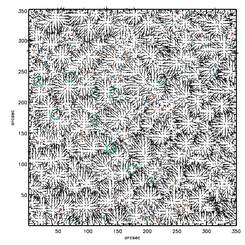
A&A 647, A178 (2021)

and magnetic concentration in the valley of the repelling LCS.         sequences and processed similarly to the Dopplergrams, except
The attractive LCS reveals the location of sinks of photospheric       for the application of the velocity filter. For the 2018 series, we
flows at supergranular junctions associated with persistent vor-       also used ultraviolet filtergrams from the Atmospheric Imaging
tices and intense magnetic flux.                                       Assembly (AIA; Lemen et al. 2012) at a wavelength of 193 Å.
    The downflows are important ingredients of the convective          The AIA sequence recorded at the original pixel size of 0.600
motions. Until now, they had only been studied only in small           was mapped to the HMI frame and tracked to coaling with HMI
fields of view and with a short cadence. The only exception            sequences.
known to us is the study by Duvall & Birch (2010), who stud-                We also used datasets from the Solar Optical Telescope
ied the vertical component of supergranulation. The downflows          (SOT; Tsuneta et al. 2008) on-board the Hinode mission space-
at mesogranular downdraft boundaries act as ‘collapsars’. Small        craft. The observations were recorded continuously on 4
granules vanish and excite the upward-propagating waves (Rast          September 2009, from 7:34:34 to 10:16:34 UT. For our study, we
1995, 1999; Skartlien & Rast 2000; Skartlien et al. 2000).             used observations of Fe i at λ = 5250 Å from the Hinode/SOT-
    The role of surface layers in the global convective simu-          NFI (Narrow band Filter Imager), where the spectral line was
lations was recently discussed by many studies. For instance           scanned at five wavelength positions along the line profile. The
Nelson et al. (2018) show that the introduction of the near-           Doppler shift at the disc centre gives us the vertical (radial) flow
surface small-scale downflows into the global 3D simulation            component vz , the Stokes V and hence the vertical component
changes the convective driving motions throughout the convec-          of the magnetic induction Bz . The pixel size of images is 0.1600
tion zone. In particular, the coalescence of downflow plumes into      and the time step is 60 s. After the flat field and dark correc-
giant cells at larger depths linked to the self-organisation of the    tions, the images were coaligned and filtered for p-modes in
near-surface plumes provides a new approach towards the con-           the k−ω space with a threshold phase velocity of 6 km s−1 .We
vection conundrum.                                                     note that arcsecond-kilometre conversion, for each dataset con-
    Today, the main difficulty seems to be the overestimation of       sidered, takes the distance between the corresponding instrument
the convective velocity in the convection zone by forward mod-         and the Sun into account.
els when forward and inverse models are compared. On the other              In order to learn about the structure of the flows also below
hand, Hotta et al. (2019) show that the surface region has an          the solar surface, we utilised time-distance local helioseismol-
unexpectedly weak influence on the deep convection zone and            ogy (Duvall et al. 1993). This method comprises tools that mea-
does not resolve the problem of the high convective velocity           sure and analyse the travel times of the waves propagating
in the deep solar interior of the state-of-the-art forward mod-        throughout solar interior.
els. Nevertheless, Hotta et al. (2019) indicate the possibility of          Travel times of the waves may be measured via cross-
an unknown influence of the unresolved small-scale turbulence.         correlations of the signals at spatially different points on the
    In this paper, we investigate the properties of near-              solar surface. Doppler shifts of the photospheric absorption lines
surface downflows through the observations of the Solar                contain clear indications about solar oscillations. We therefore
Dynamics Observatory (SDO; Pesnell et al. 2012) and Hinode             utilised HMI Dopplergrams and measured travel times using a
(Kosugi et al. 2007) satellites and finally a 3D MHD simula-           set of filters, averaging geometries and distances. Since we are
tion. In Sect. 2, we describe the data selection and reduction.        dealing with the quiet-Sun region, we measured the travel times
The analysis of the persistent downflows is presented in Sect. 3.      using linearised Gizon & Birch (2004) method.
Section 4 is devoted to the potential link between vortex and the           These travel times were then inverted for flows using multi-
persistent downflows. The non-detection of a vortex comparable         channel subtractive optimally localised averaging method (MC-
in size to observations at the surface of the Sun in the simulation    SOLA; see Jackiewicz et al. 2012) when involving the cross-talk
is described in Sect. 5. The discussion and conclusion are given       minimisation (Švanda et al. 2011; Korda & Švanda 2019). When
in Sect. 6.                                                            discussing the flows, thanks to the cross-talk minimisation our
                                                                       methodology allows one to not only infer the horizontal veloci-
2. Observations and simulation                                         ties (v x in the zonal direction and vy in the meridional direction),
                                                                       but also the vertical component vz . The inferred velocity vector
To study the properties of the medium-scale surface down-              u is a function of the horizontal position r and height z. Hori-
flows, we used two 24 h SDO Doppler observations, covering             zontal velocities are strong perturbers that may be successfully
29 November 2018, and also 2−3 November 2010. Hereafter,               retrieved to the depth, whereas the vertical velocity is a weak per-
we refer to the latter series as the ‘Requerey’s vortex’, where a      turber and only inversions in the first 1 Mm of depth are possible
strong vortical downflow was already studied by Requerey et al.        with the signal-to-noise ratio larger than one when averaging the
(2018). The regions of interest were around the disc centre in the     data over 24 h or so.
quiet-Sun regions, with a small inclination of the solar rotation           Therefore, except for the surface, the vertical velocity was
axis with respect to the observer (the heliographic latitudes of the   reconstructed from the horizontal components by integrating the
disc centre were B0 = 1.1◦ in the first case and B0 = 4.25◦ in the     equation of continuity:
second case). The original pixel size of images were 0.504000 and
0.504200 , respectively, and a time step of 45 s. Mainly, we used                               Zz0
the observations from the Helioseismic and Magnetic Imager                              −1
                                                                       vz (r0 , z0 ) =                dz ∇h · [ρ(z) uh (r0 , z)],       (1)
(HMI; Schou et al. 2012). The 24 h sequences were aligned, cor-                        ρ(z0 )
rected from the satellite motions and the limbshift, and finally                                0
tracked with the differential rotation. From the full-disc Dopp-
lergrams we extracted a region around the disc centre having           where ∇h · uh indicates the horizontal part of the velocity diver-
701 × 701 pixels on a side (35300 × 35300 ). The tracked Doppler       gence. The integration does not yield the surface vz (z = 0),
datacube was filtered in the k−ω domain with a threshold phase         where we directly use the inverted values by helioseismology.
velocity of 6 km s−1 . Line-of-sight HMI magnetograms captur-          The surface inversions for plasma flows were validated against
ing the longitudinal magnetic induction Bk were used for both          the granule-tracking inferences by Švanda et al. (2013).
A178, page 2 of 13
T. Roudier et al.: Photospheric downflows observed with SDO/HMI, HINODE, and an MHD simulation
Fig. 1. Region of interest on the 29 November 2018 datacube. The region was localised at the disc centre; the field of view has dimensions
of 35300 × 35300 . Left: 5 h mean of the HMI Dopplergrams, where black areas are considered as persistent downflows. Middle: 5 h mean of the
line-of-sight magnetic induction Bk . Right: 5 h mean of AIA 193 Å filtergrams.
For the deeper layers, we performed a set of inversions tar-
geted such that the vertical sampling was 2 Mm, starting at the
depth of 1 Mm and ending at 25 Mm. We basically followed the
vertical sampling given by Greer et al. (2016). With the depth,
the extents of the averaging kernels defining the effective reso-
lution increased monotonically, reaching 10 Mm at 1 Mm depth,
34 Mm at 13 Mm depth and finally 58 Mm at 25 Mm depth. The
vertical extent defining the vertical resolution increased as well,
having 1 Mm at the depth of 1 Mm, 2.9 Mm at the depth of
13 Mm and finally 8.7 Mm at the depth of 25 Mm.
Fig. 2. Details of Fig. 1 around one of the persistent downflows, with
a field of view of 59.500 × 73.500 . Left: mean Doppler velocity. Middle:
3. Analysis of persistent downflows with HMI, mean Bk . Right: mean AIA 193 Å filtergram.
Hinode, and simulation data
The first detection of persistent (long-lived) downflows sur-
viving for at least 4 h is described in Duvall & Birch (2010)
(their Figs. 1a and c). The results were obtained by the analy-
sis of the Dopplergrams and magnetograms from SOHO/MDI
(Scherrer et al. 1995) with a resolution of 1.200 . Duvall & Birch
(2010) selected a 4 h temporal window to average Dopplergrams
at the disc centre to follow the evolution of supergranular cells.
They tested a possible contamination of the Doppler signal by
magnetic fields but concluded that there was a rather small con-
tribution from the magnetic field. Their simultaneous 4 h aver-
age of Dopplergrams and magnetograms showed a correlation
between the persistent downflows and the magnetic induction.
We note that the persistent downflows were called apparent
downflows in their paper. Fig. 3. Coalignment of panels from Fig. 2. Background: mean
For our study, we selected a 24 h sequence of disc cen- AIA 193 Å filtergram. Blue contours: mean Bk level = 120 Gauss. Red
tre quiet-Sun Dopplergrams and magnetograms observed on 29 contours: mean Doppler velocity level = −0.2 km s−1 . Red and blue con-
November 2018 with the SDO/HMI. The spatial resolution of tours largely overlap.
these observations was 1.000 . To mimic the downflow detection
like Duvall & Birch (2010), we used the 5 h average Doppler-
grams. Figure 1 (left) convincingly shows persistent downflows downflows (red) and Bk (blue) at the exact locations relative
as localised black areas. The large amplitude of the negative to the coronal loop. In this example the persistent downflows
vertical velocity indicates that the downflow survived 24 h aver- appear to correlate with the coronal-loop anchor in the photo-
aging. These downflows with sizes around 2−300 and velocity sphere, indicating a link between the persistent downflows and
amplitudes between −0.25 and −0.72 km s−1 spatially correlate the coronal activity.
with the magnetic field in location (see the middle panel of The inspection of the 3D (x, y, t) Dopplergram datacube from
Fig. 1) and also with the regions of larger activity in the corona 29 November 2018 allowed us to detect 13 persistent down-
(images from AIA 193 Å). Figure 2 shows a zoom-out of the flows with a minimum duration of 3 h (see below). This gives
larger downflows from Fig. 1. Figure 3 displays the persistent a rate of occurrence of 2 × 10⁻⁴ cases per Mm2 and 24 h. This
A178, page 3 of 13A&A 647, A178 (2021)
Fig. 4. Top left: 24 h divergence field measured with the LCT applied to Dopplergrams. The supergranule boundaries detected by the watershed
method are shown as white network. The circles represent the location of the 13 studied a persistent downflows. These persistent downflows are
located in convergent flows and more particularly where several supergranules meet. Top right: 24 h mean Doppler map overlapped with the 13
studied persistent downflows (circles) and supergranule boundaries. Downflows are visible as dark structures in each circle. Far from the disc
centre, in the lower right part of the figure, some large darker regions are visible. These are caused by the horizontal velocities which become a
dominant contribution due to the projection effects. Bottom left: corks position (grey points) after 24 h diffusion by horizontal flows. Their locations
are, in accordance with supergranule boundaries, found by the watershed method (superimposed white network). Bottom right: 24 h mean magnetic
field and the location of the 13 studied persistent downflows (circles).
rate is lower than those found by Requerey et al. (2017) during boundaries plotted over the divergence field are shown as a
sequences of 32.0 and 22.7 min of 6.7 × 10⁻² per Mm2 . These white network in Fig. 4 (top left). In Fig. 4 (top right) the
two rates of occurrence are not directly comparable because the 24 h mean Doppler map is overlapped by locations of the 13
first one deals with very long-lasting downflows (a few hours) studied persistent downflows (circles) and supergranular bound-
although the second rate is related to shorter-lasting downflows aries. Downflows are visible as dark structures in each circle.
(30 min). The persistent downflows are identified in the convergent flows
To detect the supergranule boundaries, horizontal velocities and more particularly at positions, where several supergran-
were computed with the local correlation tracking technique ules meet. This is in agreement with the conclusion that vortex
(LCT; November 1986) applied to the sequence of Doppler- flows are usually located at supergranular junction vertices found
grams. From the derived horizontal velocities, we computed by Attie et al. (2009, 2016). Using the 24 h horizontal-velocity
the 24 h average divergence field and the supergranule bound- fields, we computed the corks diffusion during that period of
aries using the watershed method (Roudier et al. 2020). These time. Figure 4 (bottom left) confirms that the locations of the
A178, page 4 of 13T. Roudier et al.: Photospheric downflows observed with SDO/HMI, HINODE, and an MHD simulation
Fig. 5. Doppler (top) and magnetic (bottom) temporal
cuts centred on the 13 selected persistent downflows.
The time (vertical axis) stands for 24 h, the spatial axis
(y cut, horizontal) is 1500 for each column and the num-
bers indicate the labels of the selected downflows cor-
responding to the bottom right of Fig. 4. The persistent
downflows move across the surface but are visible in the
cuts at least from 3.5 h to 20 h.
persistent downflows and the magnetic field is well observed and
conforms to the one found by Duvall & Birch (2010). The mag-
netic field is always observed at the location of the persistent
downflows. From our set, only one persistent downflow (num-
ber 6) seems to be without a strong magnetic counterpart (see
bottom right panel of Fig. 4).
To quantify the velocity-magnetic field correlation, we plot-
ted the mean Doppler velocity versus Bk from the 24 h sequence
in Fig. 6. In the regions where Bk > 60 G, a linear relationship
between the magnetic field and the observed Doppler velocity is
most clear as described by Duvall & Birch (2010). The strongest
magnetic concentrations are found in the strongest downflows.
As we observe with high-resolution HMI data (0.500 per pixel),
Fig. 6. Scatter plot of the dependence of Doppler velocity and Bk
the positive correlation probably indicates a suppression of the
obtained for the SDO data on 29 November 2018.
granular flows due to the magnetic field. Our observations thus
confirm the hypothesis by Duvall & Birch (2010).
persistent downflows (circles) at the supergranule boundaries are
situated where the corks are accumulate. 3.1. Depth structure of the persistent downflows
Temporal cuts of the Doppler velocities centred on the 13
persistent downflows are shown in Fig. 5 (top). The downflows The persistent downflows identified in the HMI frame were also
are visible as dark structures in the cuts and they last for a long localised in the helioseismic datacubes. Unlike full-resolution
time from 3.5 h to 20 h in our examples. However, the downflows Dopplergrams or velocity fields obtained by LCT, the helioseis-
move across the surface during their lifetimes which makes it mic inferences have a much coarser spatial resolution, 10 Mm
difficult to catch them on single positional cuts. Nevertheless, the effective resolution at the surface at best. Therefore these spa-
Doppler temporal cuts clearly exhibit their long duration. Some tially confined persistent downflows cannot be directly identi-
of them are not fully continuous but are visible at the same posi- fied in the helioseismic frames. We verified that no clear signal
tion. The sizes of these downflows are around 2−300 . of these confined downflows is present in the travel-time maps.
Figure 5 (bottom) shows magnetic field temporal cuts cen- This is due to the fact that the typical wavelength of the p-modes
tred on the 13 persistent downflows. The correlation between the and the surface gravity f -modes is a few megametres, which is
A178, page 5 of 13A&A 647, A178 (2021)
Fig. 8. Example vertical cut through the 3D vertical velocity at y =
21000 .
eight out of 13 cases all the way to the bottom of the domain of
interest.
These 13 selected persistent downflows are not the only
downflows present in the field of view. By doing an automatic
search we identified 183 downflows in the region of interest as
the local minima of the vertical velocity which, at the same time,
exhibited the negative value. From those downflows we selected
the 13 strongest to represent a comparative set to the 13 per-
sistent downflows. For each of the three sets, we computed the
average vertical flow profile in the centre of the downflow. These
plots are given in Fig. 10. We note that our results are only
weakly influenced by the downflow changing the position in the
coordinate frame, as these positional changes are rather small
(about 500 ). These positional changes are significantly smaller
Fig. 7. Locations of the 13 selected downflows (open circles) on vertical than the effective resolution of the helioseismic flow maps (about
velocity map at the surface (top) and at the depth of 25 Mm (bottom). 1300 at the surface, the number increases with depth).
The flows were averaged over 24 h on the day of 29 November 2018. There is an obvious difference between the common and
the persistent downflows. The persistent downflows, on average,
may have a smaller amplitude both at the surface and in the near-
surface layers, but on average the flows remain negative all the
much larger than the horizontal extent of the identified persistent way to the bottom of our inversion domain. Compared to that
downflows. the average over all common downflows tends to be zero at the
Hence, the downflows were localised by their coordinates. In depth of about 8 Mm and remains negligible further down. The
Fig. 7 we see their locations on the vertical-flow maps derived comparative set of the strongest downflows has a much larger
at the surface (a helioseismic inversion) and at the depth of magnitude peaking at the depth of about 3 Mm on average, but it
25 Mm (estimate obtained from integrating Eq. (1)). At the sur- reaches zeros at the depth of about 13 Mm on average and deeper
face frame the locations of the persistent downflows do not seem down it even turns positive.
to be special except that they are mostly located at the edges
of supergranules. On the other hand, at a depth of 25 Mm most 3.2. Persistent downflows in 2 h 30 min Hinode observations
of them seem to be present at locations of the negative vertical
velocity or very close to it. As a complementary series, we analysed the 2 h 30 min series of
Vertical cuts through vertical velocity generally show a com- Dopplergrams (based on Fe i at λ = 5250 Å line) and the lon-
plicated structure (see an example in Fig. 8). In most cases, it gitudinal magnetic field. SOT/NFI on-board Hinode has a spa-
is not possible to track the downflows or upflows through the tial resolution of 0.3500 . Two examples of persistent downflows
datacube in a depth strictly vertically. In some cases the verti- found in the datacube sequences are displayed in Fig. 11. There,
cal velocities create compact regions that are shifted laterally in in the top row, we see an average of the Doppler and Bk over 2 h
between the consecutive depths. Merging of the downflows and 30 min. In the bottom row, the cuts in the (x, t) and (y, t) planes
separation of the upflows are visible in the cuts. through Dopplergram and Bk datacubes are plotted at the cen-
In this study, we did not focus on a general analysis of down- tres of the two persistent downflows. Here, the persistent down-
flows, we rather studied the 13 representatives that prevailed for flows are clearly associated with the presence of the magnetic
a long time and were associated with the magnetic elements. The field. The relationship between the magnetic field and the down-
vertical cuts through these downflows are seen in Fig. 9. As one flows (Fig. 12) is identical to that obtained with the SDO data.
can see, in most cases the downflow seems to be present deep, in It is important to note that the amplitude of the magnetic field
A178, page 6 of 13T. Roudier et al.: Photospheric downflows observed with SDO/HMI, HINODE, and an MHD simulation
Fig. 9. Vertical cuts through the vertical velocity around
the 13 selected downflows from 29 November 2018.
Around each downflow, a vicinity of 2000 was segmented
and the cut was plotted in both zonal and meridional
directions.
tions from the Hinode satellite. In the literature, the terms ‘vor-
tex’ and ‘swirl’ are both employed to identify rotating structures
in the flows. A large review of the vortex (or swirls) detection
is given in Murabito et al. (2020). Photospheric vortex flows are
usually correlated with a network of magnetic elements at super-
granular vertices (Requerey et al. 2018).
4.1. Vortex detection
Here, medium spatial resolution observations are used over a
larger field of view to detect a potential vortex (or swirls).
From the horizontal velocity field, we applied the vortex detec-
tion to identify ‘swirls’ as described in Giagkiozis et al. (2017),
de Souze e Almeida Silva et al. (2018), Liu et al. (2019), with
Fig. 10. Average depth profiles of the vertical flows in downflows. The the two dimensionless parameters Γ1 (P) and Γ2 (P) at the target
dashed line represents the average over all 183 downflows located in the point P:
field of view. The dot-dashed line is an average over the 13 strongest (at
1 X nPM × uM
the surface) downflows in the region. The solid line then shows the plot Γ1 (P) = , (2)
for the 13 persistent downflows. N M∈S kuM k
1 X nPM × (uM − uP )
Γ2 (P) = , (3)
is lower in the Hinode data, which is due to the smaller field of N M∈S kuM k − uP
view and a quieter region.
where uM and uP are the velocity vectors at the points M and P, S
is the two dimensional region with the size N pixels surrounding
4. Link between persistent downflows and potential the target point P, M is the point within the region S , nPM is the
vortex normal vector pointing from P to M, and × stands for the vector
product (Liu et al. 2019).
Requerey et al. (2018) analysed a long-lived and large vortex Here for convenience, we use only the term vortex and the
(having a size of about 5 Mm) using high spatial (0.200 ) observa- parameter Γ1 to detect the core of a vortex. More sophisticated
A178, page 7 of 13A&A 647, A178 (2021)
Fig. 13. Γ1 computed from 24 h mean velocity overlapped by horizontal
velocity field. Blue and red represent counter clockwise and clockwise
velocities respectively. The locations of the 13 studied persistent down-
flows are indicated by circles.
ative to the measured Γ1 parameter computed with the 24 h mean
velocity field. In that figure only a few of the 13 downflows
correspond to the detected vortex (here via Γ1 > 0.5). How-
Fig. 11. Two persisting downflows during 2 h 30 min of Hinode obser- ever, a detailed inspection reveals a vorticity, at least, in six of
vations. Top: averaged Dopplergrams and Bk around two different per- them (46%) (downflows 1, 2, 4, 5, 8, and 13) during a portion
sistent downflows in a field of view of 4.400 × 4.400 . Middle: cuts around of their lifetimes, including 9.9 h–17.3 h, 0.9 h–7.1 h, 10.9 h–
the persistent downflows in the (y, t) plane of the Dopplergram and Bk 18.1 h, 10.7 h–19.7 h, and 10.9 h–16.3 h, respectively. Examples
datacubes. The dimensions of the arrays are (4.400 × 2 h 30 min). Bot- of downflows number 5 and 8 are given in the figure.
tom: same in the (x, t) plane. Figure 14 shows the mean Doppler and |Γ1 | > 0.4 parame-
ter for the two periods of time relative to the beginning of the
sequence: 11.4 h–15.2 h and 15.4 h–19.7 h of downflow num-
ber 5. The temporal evolution of the flows indicates, very close to
the downdraft, a direction change in the vortex rotation. There-
fore, the vortex direction seems to be very sensitive to the evo-
lution of local large-amplitude flows and can be reversed as in
our example. Another vortex is presented in Fig. 15, where we
observe a clear link between |Γ1 | > 0.23 and persistent down-
flow number 8. One important point is that we never detect a
vortex before the appearance of the magnetic field in the down-
flow, when it is possible to observe that in a few cases. We do
not know if this is due to the 100 of spatial resolution and 45 s
temporal step.
Fig. 12. Correlation between Bk and the Doppler velocity of the mean 4.2. Requerey’s vortex and long-lived downflows
data 2 h 30 min of the mean Hinode data.
To validate our vortex detection via the parameters Γ1 and
Γ2 , we used the SDO observation used in the analysis of
vortex detection have been recently developed (LCS approach; Requerey et al. (2018), de Souze e Almeida Silva et al. (2018),
see de Souze e Almeida Silva et al. 2018 or Chian et al. 2019) Chian et al. (2019). Luckily, SDO observations started just
but our small sample allows us to control the vortex detection before Requerey’s observations were made with the Hin-
by eye. For an ideal vortex, Γ1 (P) is maximum (value is equal to ode satellite. We remind the readers that Requerey et al.
1) at the centre of the vortex and decreases towards zero outside (2018), de Souze e Almeida Silva et al. (2018), Chian et al.
of it. Hence, it allows us to determine both the vortex location (2019) observed and analysed a nice long-lasting vortex. The
and the radius. Figure 13 shows the 13 persistent downflows rel- advantage of the SDO observations is the access to various kinds
A178, page 8 of 13T. Roudier et al.: Photospheric downflows observed with SDO/HMI, HINODE, and an MHD simulation
Fig. 14. Top: mean Doppler downflow number 5
from time 11.4 h to time 15.2 h (left) and from
time 15.2 h to 19.7 h (right) relative to the begin-
ning of the sequence, overlapped with the mean
horizontal velocities. Bottom: vorticity charac-
terised by the |Γ1 | > 0.4 parameter (downflow
number 5) from time 11.4 h to 15.2 h (left) and
from time 15.2 h to 19.7 h (right), overlapped
with the mean horizontal velocities. White and
black represent counter-clockwise Γ1 and clock-
wise velocities, respectively.
Fig. 15. Left: mean Doppler downflow num-
ber 8 between time 5 h and 10.7 h over-
lapped with the mean horizontal velocities.
Right: vorticity characterised by the |Γ1 | >
0.5 parameter (downflow 8). White and black
represent counter-clockwise Γ1 and clockwise
velocities, respectively.
of context observations, on the same day, to a larger field of have vorticity but also a non-negligible shear component which
view. Despite the spatial resolution of SDO being lower than that contributes to the final amplitude of Γ1 and hence does not allow
of Hinode, we detected the vortex described in Requerey et al. for one to call them a vortex. However, Chian et al. (2019, 2020)
(2018) without any problem. The locations of Γ1 , vortex detec- with higher spatial resolution, reported on the same field of view,
tion overlapped by a horizontal velocity field are plotted in more persistent objective vortices with shorter lifetimes corre-
Fig. 16. The Requerey’s vortex is well detected by the gamma- sponding to the gap regions of ‘Lagrangian chaotic saddles’.
method and is clearly visible in the plotted horizontal veloci- In the larger field of view, the horizontal velocity module
ties (at the coordinates (6200 × 4900 ). Figure 17 shows the mean (Fig. 18) shows, in the central part, the roundish supergran-
Doppler overlapped by horizontal velocity field and the location ule corresponding to the supergranule shown in Fig. 16, where
of the Γ1 corresponding to downflows around the supergranule. Requerey’s vortex is observed. This supergranule is a particu-
In our observations, five larger-amplitude regions in the Γ1 larly symmetrical, well-formed supergranule with large ampli-
parameter are seen in total (see Figs. 16 and 17) and only one of tude horizontal outflows. The large horizontal velocity amplitude
them corresponds to the vortex studied by Requerey. The others of that supergranule and the combination of the velocities from
A178, page 9 of 13A&A 647, A178 (2021)
Fig. 18. Requerey’s vortex in a large field of view of the module of the
Fig. 16. Γ1 ‘vortex’ (in circles) overlapped by horizontal velocity field. mean horizontal velocities (24 h mean).
Fig. 17. Mean Dopplergram overlapped by horizontal velocity field and
the location of the Γ1 ‘vortex’ (in circles).
Fig. 19. Persisting downflows during 24 h. (y, t) cuts through the Dopp-
lergram (left) and Bk (right). Requerey’s vortex corresponds to the long-
lasting downflow and Bk is located around y ≈ 12000 .
the large supergranules on its right location on the eastern edge,
produce the large Requerey’s vortex. The temporal and spatial
coincidence is probably the reason for producing this large and
of 20 Mm and more (see Fig. 20). The plotted profile is similar
long-lasting vortex. The other large amplitude downflows around
to the profile of the strongest downflows recorded in the studied
this supergranule do not show identical properties (see Fig. 19).
field of view on 29 November 2018 (compare to the dash-dotted
Helioseismic inversion allows us to study the general prop-
line in Fig. 10).
erties of the large Requerey’s vortex in depth. In the map of the
In the maps of the vertical vorticity computed from the hori-
inverted component, nothing extraordinary is seen at the loca-
zontal flow components as
tion of this vortex, likely because the spatial resolution of the
flow maps is again coarser than the extent of the vortex. The
plot of the vertical profile of the vertical velocity, on the other ∂v x ∂vy
hand, clearly shows that the downflow extends deep into depth Ωz = − , (4)
∂y ∂x
A178, page 10 of 13T. Roudier et al.: Photospheric downflows observed with SDO/HMI, HINODE, and an MHD simulation
10 The first dataset provides the velocity vector u(x, y, t) and the
magnetic field vector B(x, y, t) over the solar surface (z = 0)
0 for 27 h (spatial resolution: 96 km pixel−1 ; temporal resolution:
60 s; field of view (FOV): 96 Mm × 96 Mm). The corresponding
resolution is 0.1300 on the Sun, as the computational pixel size
−10
is 48 km, which is much better than observations. We used the
v x , vy , vz as well as Bz quantities. The z axis is positive above
−20
vz [m/s]
the surface. The second dataset, which is much shorter, gives
only the vertical velocity vz (x, y, z, t) during 4 h from the surface
−30 (z = 0) to z = −20 Mm, with the same horizontal FOV and time
step as the first dataset.
−40 In order to eliminate 5 min oscillations, the vertical velocity
field vz was filtered in the k−ω diagram low frequencies such
−50 that ω < c k were kept and other frequencies were eliminated
(c = 6 km s−1 ). Then, we averaged velocities and magnetic fields
−60 over time intervals 12 and 24 h for the first sequence close to
0 5 10 15 20 25 the supergranulation lifetime and 4 h for the second sequence in
Depth [Mm]
order to keep only long-lasting features.
Fig. 20. Depth profile of the 24 h averaged vertical velocity in the mid- Figure 22 displays 12 h averages (first dataset) of the vertical
dle of Requerey’s vortex. magnetic field Bz and the divergence of the horizontal veloci-
ties vh = (v x , vy ). The long-duration downflows (red points) are
−5
spatially much more concentrated and also much more numer-
x 10 ous than in observations. They occur almost everywhere, even
6
in non-magnetic areas. Such points are systematically charac-
terised by ∇h · uh < 0 (converging flows) with the mean value
5
of −1.8 × 10⁻³ s−1 . The second dataset shows that these points
are also characterised by dvz /dz > 0 at z = 0, which means that
4 the amplitude of vz decreases with height in these points at the
surface. The mean value is 1.9 × 10⁻³ s−1 , so that we are close to
3 ∇ · u = 0 at the surface. Therefore, the fluid exhibits an uncom-
Ωz [1/s]
pressible behaviour in this layer.
2 Figure 23 shows two typical cross sections of the vertical
flows based on the second dataset, averaged over 4 h. Some
1 downflows extend from the surface down to z = −13 Mm. How-
ever, most downflows are not deeper than z = −4 Mm. We also
0
point out that the continuous downflow regions do not extend
purely vertically to a certain depth, but they depict a lateral dis-
placement between the depths. This behaviour is very similar to
−1 what we found in the helioseismic inversions (cf. Fig. 8).
0 5 10 15 20 25
Depth [Mm] We conclude that the numerical simulation predicts the exis-
tence of spatially concentrated lasting downflows in the quiet
Fig. 21. Depth profile of the vertical component of the flow field vortic-
Sun with a typical size of about 0.2500 . However, the spatial res-
ity in the middle of Requerey’s vortex.
olution of observations used in this paper does not allow us to
confirm simulation results. In the simulations, we did not find
Requerey’s vortex is clearly visible. The depth profile of Ωz evidence of a vortex comparable in size to the observed vortex
shows that the vorticity keeps its integrity to the depth of about on the surface of the Sun.
5 Mm (see Fig. 21), where it seems to start to oscillate around
zero and vanishes at the depth of about 11 Mm. We do not think 6. Results and conclusion
that the peak at the depth of 9 Mm that is visible in both vertical
velocity and vertical vorticity profiles is particularly real. The The properties of solar plasma below the surface is mostly
formal uncertainty of the vertical velocity at this depth is about inferred from the observations of solar surface oscillations.
10 m s−1 and that of the vertical velocity vorticity about 10−5 s−1 , The formation of vigorous downflowing plumes and the
which corresponds to the magnitude of these ‘peaks’. The com- collective interaction of these (Rast 2003; Cossette & Rast
parison of Requerey’s vortex and the downflows in the field of 2016) also provides the opportunity, combined with local
view on 29 November 2018 indicates that the long-living vortex helioseismology, to probe the first megameters of the
is linked to strong downflows. solar interior. Lot of observations of vortices (vortex)
associated with downflows are described in the literature
(Attie et al. 2009, 2016; Duvall & Birch 2010; Bonet et al. 2010;
5. Simulation link between magnetic field and Vargas Domínguez et al. 2011, 2015; Requerey et al. 2017,
persistent downflows 2018), generally studied on short sequences. Three of them
are observed on long temporal sequences from 4 h to 24 h
We used two different datasets based on the 3D MHD numer- (Attie et al. 2009, 2016; Duvall & Birch 2010; Requerey et al.
ical simulation. These runs apply to the purely quiet Sun 2018). Taking advantage of the long temporal and homoge-
(Stein & Nordlund 1998). neous SDO/HMI observations (24 h here) of the Dopplergrams
A178, page 11 of 13A&A 647, A178 (2021)
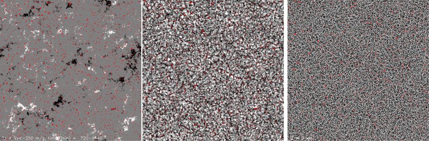
Fig. 22. Bz , ∇h · uh , ∇vz at the surface (FOV 96 × 96 Mm2 ). Long-lasting downward velocities are displayed as red points using the threshold of
−0.25 km s−1 . Left: Bz (grey levels), averaged over 12 h. Middle: ∇h · uh averaged over 12 h. Bright and dark correspond to diverging and converging
flows, respectively. Right: dvz /dz averaged over 4 h. Bright and dark correspond to upward and downward vertical gradient, respectively.
Fig. 23. Cross sections of the vertical velocity vz (in x × z and y × z planes) at pixel (x = 171 Mm, y = 452 Mm) indicated by the vertical lines, where
a typical downflow occurs. The surface is at z = 0 Mm. Bright and dark correspond to upflows and downflows, respectively.
and magnetograms, we investigate the properties of the down- with an observed vortex, but not all the time and not for all
flows, particularly the long-lasting one called persistent down- the studied downflows. At higher spatial resolution (Chian et al.
flows here, and their links to a concentrated magnetic field and 2019, 2020), more persistent objective vortices were found with
finally the link with the corona observations (AIA 193 Å). shorter lifetimes corresponding to the gap regions of ‘Lagrangian
In the 3D data cube (x, y, t) of the 24 h Doppler sequence chaotic saddles’.
(29 November 2018), at the disc centre, we detect 13 persistent All the studied persistent downflows are always associated
downflows giving a rate of occurrence of 2×10⁻⁴ cases per Mm2 with a magnetic field (up to 600 Gauss). No significant down-
and 24 h. This rate is lower than those found by Requerey et al. flows were observed before the appearance of the magnetic field
(2017) during sequences of 32.0 and 22.7 min of 6.7 × 10⁻² as described in Vargas Domínguez et al. (2015). The advantage
per Mm2 which was found with higher spatial resolution but on of their higher spatial resolution (0.1500 ) probably allows them to
shorter time sequences. The lifetimes of our 13 persistent down- detect downflows before the magnetic field appearance and fol-
flows were found between 3.5 h to and 20 h with a sizes between low the enhancement of this magnetic field by the strong down-
2 and 300 and speeds between −0.25 and −0.72 km s−1 . They are flows. The detection of the vortex described by Requerey et al.
well located at the junction of several supergranules as observed (2018) with our SDO/HMI data gives confidence in our method
by Attie et al. (2009, 2016), Chian et al. (2019, 2020). In our of vortex detection. This very beautiful vortex, with our large
examples, only 46% of the persistent downflows were connected field of view, seems to be the result of the composition of the
A178, page 12 of 13T. Roudier et al.: Photospheric downflows observed with SDO/HMI, HINODE, and an MHD simulation
larger-scale horizontal flows where the combination of the flow Bello González, N., Yelles Chaouche, L., Okunev, O., & Kneer, F. 2009, A&A,
phases, temporal and spatial, creates it. 494, 1091
We observe that this downflow is always associated with the Berger, T. E., Rouppe van der Voort, L. H. M., Löfdahl, M. G., et al. 2004, A&A,
428, 613
presence of the magnetic field. The helioseismic inversion allows Bonet, J. A., Márquez, I., Sánchez Almeida, J., Cabello, I., & Domingo, V. 2008,
us to describe the persistent downflow properties in depth below ApJ, 687, L131
the solar surface and, for instance, to compare the properties of Bonet, J. A., Márquez, I., Sánchez Almeida, J., et al. 2010, ApJ, 723, L139
the persistent downflows to the other (non-persistent) in the field Chian, A. C.-L., Silva, S. S. A., Rempel, E. L., et al. 2019, MNRAS, 488, 3076
Chian, A. C.-L., Silva, S. S. A., Rempel, E. L., et al. 2020, Phys. Rev. E, 102,
of view. Persistent downflows seem to penetrate deeper, whereas 060201
the common downflows seem to reach zero vertical velocity Cossette, J.-F., & Rast, M. P. 2016, ApJ, 829, L17
already at the depth of around 7 Mm. The persistent downflows de Souze e Almeida Silva, S., Rempel, E. L., Pinheiro Gomes, T. F., Requerey, I.
remain slightly negative on average all the way to the bottom of S., & Chian, A. C. L. 2018, ApJ, 863, L2
our region of interest, which is 25 Mm. Duvall, T. L., Jr., & Birch, A. C. 2010, ApJ, 725, L47
Duvall, T. L., Jr., Jefferies, S. M., Harvey, J. W., & Pomerantz, M. A. 1993,
In the high spatial resolution MHD simulation (0.1300 ), long- Nature, 362, 430
duration downflows (4 h and 12 h) are spatially much smaller and Giagkiozis, I., Fedun, V., Scullion, E., & Verth, G. 2017, ArXiv e-prints
numerous than in observations where the resolution lies around [arXiv:1706.05428]
2 to 300 . We did not find evidence of a vortex comparable in size Gizon, L., & Birch, A. C. 2004, ApJ, 614, 472
Greer, B. J., Hindman, B. W., & Toomre, J. 2016, ApJ, 824, 128
to observations. The spatial resolution of observations does not Hanasoge, S. M., & Sreenivasan, K. R. 2014, Sol. Phys., 289, 3403
allow us to see small scale downflows, so that observations with Hotta, H., Iijima, H., & Kusano, K. 2019, Sci. Adv., 5, 2307
more precise satellites (as the PHI on-board Solar Orbiter) or Innes, D. E., Genetelli, A., Attie, R., & Potts, H. E. 2009, A&A, 495, 319
ground-based large telescopes are required. Jackiewicz, J., Birch, A. C., Gizon, L., et al. 2012, Sol. Phys., 276, 19
From the space-borne SDO instruments, downflow evolu- Korda, D., & Švanda, M. 2019, A&A, 622, A163
Kosugi, T., Matsuzaki, K., Sakao, T., et al. 2007, Sol. Phys., 243, 3
tion is studied at different wavelengths. We observe a persis- Lemen, J. R., Title, A. M., Akin, D. J., et al. 2012, Sol. Phys., 275, 17
tent downflow to be correlated with the coronal-loop anchor Liu, J., Nelson, C. J., & Erdélyi, R. 2019, ApJ, 872, 22
in the photosphere, indicating a link between downflows and Murabito, M., Shetye, J., Stangalini, M., et al. 2020, A&A, 639, A59
the coronal activity. This observation is to be compared with Narayan, G. 2011, A&A, 529, A79
Nelson, N. J., Featherstone, N. A., Miesch, M. S., & Toomre, J. 2018, ApJ, 859,
the observed EUV cyclones over the quiet Sun, anchored in 117
the rotating magnetic field network magnetic fields, suggesting November, L. 1986, J. Appl. Opt., 25, 392
an effective way to heat the corona Zhang & Liu (2011). The Pesnell, W. D., Thompson, B. J., & Chamberlin, P. C. 2012, Sol. Phys., 275, 3
link between the flow evolution at the junctions of supergranu- Rast, M. 1995, ApJ, 443, 863
lar cells, giving mini-coronal-mass ejection and X-ray network Rast, M. P. 1999, ApJ, 524, 462
Rast, M. P. 2003, ApJ, 597, 1200
flares, is described in Innes et al. (2009), Attie et al. (2016). Requerey, I. S., Del Toro Iniesta, J. C., Bellot Rubio, L. R., et al. 2017, ApJS,
Hence, the persistent downflows must be investigated with a 229, 14
greater number of time sequences.In the same way, more stud- Requerey, I. S., Cobo, B. R., Gošić, M., & Bellot Rubio, L. R. 2018, A&A, 610,
ies have to be performed on the link between persistent down- A84
Rieutord, M., & Zahn, J. P. 1995, A&A, 296, 127
flows and the coronal phenomena to confirm the link between Rincon, F., & Rieutord, M. 2018, Liv. Rev. Sol. Phys., 15, 6
them and describe the temporal dynamic behaviour of such Roudier, T., Malherbe, J. M., Gelly, B., et al. 2020, A&A, 641, A50
structures. Scherrer, P. H., Bogart, R. S., Bush, R. I., et al. 1995, Sol. Phys., 162, 129
The new non-linear methods (Lagrangian Coherent Struc- Schou, J., Scherrer, P. H., Bush, R. I., et al. 2012, Sol. Phys., 275, 229
ture and Lagrangian Chaotic Saddles) developed recently by Skartlien, R., & Rast, M. P. 2000, ApJ, 535, 464
Skartlien, R., Stein, R. F., & Nordlund, Å. 2000, ApJ, 541, 468
Chian et al. (2019, 2020), applied to the full Sun SDO/HMI Stein, R. F., & Nordlund, Å. 1989, ApJ, 342, L95
observations, is probably the best way for future research in this Stein, R. F., & Nordlund, Å. 1998, ApJ, 499, 914
domain to access to large-events statistics. Stein, R. F., Nordlund, Å., Georgoviani, D., Benson, D., & Schaffenberger, W.
2009, in Solar-Stellar Dynamos as Revealed by Helio- and Asteroseismology:
Acknowledgements. This work was granted access to the HPC resources of GONG 2008/SOHO 21, eds. M. Dikpati, T. Arentoft, I. González Hernández,
CALMIP under the allocation 2011-[P1115]. Thanks to SDO/HMI, IRIS, and C. Lindsey, & F. Hill, ASP Conf. Ser., 416, 421
Hinode/SOT teams. MŠ and DK were supported by the Czech Science Founda- Švanda, M., Gizon, L., Hanasoge, S. M., & Ustyugov, S. D. 2011, A&A, 530,
tion under the grant project 18-06319S. A148
Švanda, M., Roudier, T., Rieutord, M., Burston, R., & Gizon, L. 2013, ApJ, 771,
32
References Tsuneta, S., Ichimoto, K., Katsukawa, Y., et al. 2008, Sol. Phys., 249, 167
Vargas Domínguez, S., Palacios, J., Balmaceda, L., Cabello, I., & Domingo, V.
Attie, R., Innes, D. E., & Potts, H. E. 2009, A&A, 493, L13 2011, MNRAS, 416, 148
Attie, R., Innes, D. E., Solanki, S. K., & Glassmeier, K. H. 2016, A&A, 596, Vargas Domínguez, S., Palacios, J., Balmaceda, L., Cabello, I., & Domingo, V.
A15 2015, Sol. Phys., 290, 301
Belkacem, K., Samadi, R., Goupil, M. J., & Kupka, F. 2006, A&A, 460, 173 Zhang, J., & Liu, Y. 2011, ApJ, 741, L7
A178, page 13 of 13You can also read