An electrostatics method for converting a time series into a weighted complex network
←
→
Page content transcription
If your browser does not render page correctly, please read the page content below
www.nature.com/scientificreports
OPEN An electrostatics method
for converting a time‑series
into a weighted complex network
Dimitrios Tsiotas1,2,3*, Lykourgos Magafas3 & Panos Argyrakis3,4
This paper proposes a new method for converting a time-series into a weighted graph (complex
network), which builds on electrostatics in physics. The proposed method conceptualizes a time-series
as a series of stationary, electrically charged particles, on which Coulomb-like forces can be computed.
This allows generating electrostatic-like graphs associated with time-series that, additionally to the
existing transformations, can be also weighted and sometimes disconnected. Within this context,
this paper examines the structural similarity between five different types of time-series and their
associated graphs that are generated by the proposed algorithm and the visibility graph, which is
currently the most popular algorithm in the literature. The analysis compares the source (original)
time-series with the node-series generated by network measures (that are arranged into the node-
ordering of the source time-series), in terms of a linear trend, chaotic behaviour, stationarity,
periodicity, and cyclical structure. It is shown that the proposed electrostatic graph algorithm
generates graphs with node-measures that are more representative of the structure of the source
time-series than the visibility graph. This makes the proposed algorithm more natural rather than
algebraic, in comparison with existing physics-defined methods. The overall approach also suggests a
methodological framework for evaluating the structural relevance between the source time-series and
their associated graphs produced by any possible transformation.
The multidisciplinary nature of n etworks1–3 has introduced new directions in the time-series research that led
to the emergence of the complex network analysis of time-series. This newly established research field showed
a remarkable development, at a multidisciplinary level4, when scholars c onceptualized5–7 that transforming a
time-series into a graph can produce insights that are not visible by current time-series approaches. In general,
studying the topology of a graph instead of the structure of a time-series promotes time-series analysis because
it enlarges the embedding of the available information, from a first-order tensor (i.e. the time-series vector)
into a second-order tensor (i.e. the graph connectivity matrix)8. Within this context, Zhang and S mall7 were
the first who constructed graphs from pseudo-periodic time-series, and Yang and Y ang6 applied thresholds to
9
the correlation matrix to convert it into a connectivity matrix. Xu et al. proposed a transformation for creating
graphs from time-series based on different dynamic systems. Lacasa et al.5 built on the intuition of considering
a time-series as a landscape and introduced a connectivity criterion based on visibility from optics physics. Gao
and Zin10 proposed methods (i.e. flow pattern complex network, dynamic complex network, and fluid–struc-
ture complex network) to construct complex networks from experimental flow signals, and Donner et al.11
introduced a recurrence method converting graphs from time-series based on the phase-space of a dynamical
system. Amongst the existing methods, the natural visibility graph (NVG) or, in synonym, the visibility graph
algorithm (VGA) of Lacasa et al.5 seems to prevail in the literature either in terms of citations, or in the number
of applications12–14, or the number of derivative methods, such as the horizontal visibility graph of Luque et al.15,
and the visibility expansion algorithm of Tsiotas and C harakopoulos8,16. The popularity of VGA can be either due
to its intuitive conceptualization from optics physics, which makes comprehension and interpretation of results
easier, or to its topological consistency to convert periodic time-series to regular graphs, random time-series to
random graphs, and fractal time-series to scale-free graphs. However, this method builds on a binary connectivity
criterion, which leads to the development of binary connections and thus to unweighted g raphs5. Therefore the
VGA is by definition restricted in generating visibility graphs that are disassociated from the numerical scale of
the source (original) time-series.
1
Department of Regional and Economic Development, Agricultural University of Athens, Amfissa, Greece. 2Adjunct
Academic Staff, School of Social Sciences, Hellenic Open University, 10677 Athens, Greece. 3Laboratory of
Complex Systems, Department of Physics, International Hellenic University, Kavala, Greece. 4Department of
Physics, Aristotle University of Thessaloniki, Thessaloniki, Greece. *email: tsiotas@aua.gr
Scientific Reports | (2021) 11:11785 | https://doi.org/10.1038/s41598-021-89552-2 1
Vol.:(0123456789)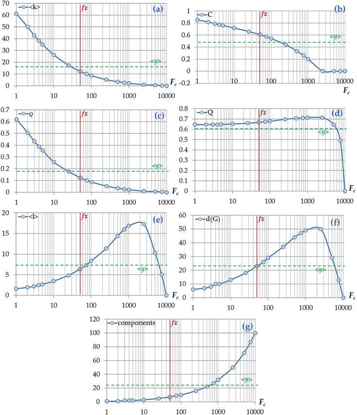
www.nature.com/scientificreports/
Figure 1. Example of the electrostatic graph (ESG) algorithm conceptualization. The volume of electrical
charge (qi, i = 1,..,8) in each node is shown proportionally to the node size (xi, i = 1,..,8) of the time-series.
Aiming at serving the demand of promoting a weighted conceptualization in the complex network analysis
of time-series, this paper introduces a method for converting a time-series into a weighted graph by using an
electrostatics transformation algorithm based on Coulomb’s law. The proposed method is driven by a dual moti-
vation: the first builds on the example of the V GA5, which implies that physics-defined transformations can be
more intuitive and easily comprehensive than the algebraic (or computational) ones. The second one is based
on the universality of Coulomb’s inverse square l aw17, which grounded the development of essential research in
electromagnetism but also inspired multidisciplinary research in e conomics18, urban and spatial planning and
transport engineering19,20, biology21, geophysics22, computational23 and communication sciences24, etc. Within
this multidisciplinary context, the proposed method conceptualizes a time-series as a sequence of stationary
and electrically charged particles (nodes) and generates an electrostatic graph based on pair-wise calculations of
Coulomb’s law across the time-series nodes. The Coulomb-like forces are assigned as weights in the connectiv-
ity matrix of the electrostatic graph and can be seen as a measure of relevance between two nodes, in terms of
the sign, scale, and spatial proximity. This approach allows quantifying the interaction between the time-series
nodes and thus to conceptualize the dynamics of a time-series through the effect of electrostatic forces applied
between the nodes.
The remainder of the paper is organized as follows: Sect. 2 (methods) describes the proposed ESG algorithm
and its modeling context, it introduces the node-series of network measures concept in the ESG, and it briefly
describes the methods used for testing the performance of the proposed algorithm. Section 3 (Results) shows
the results of the multilevel analysis testing the performance of the proposed algorithm in comparison with a
well-established method of converting a time-series to a graph. Finally, in Sect. 4, conclusions are given.
Methods
The proposed ESG algorithm. Let us consider a time-series X = {x1, x2,…, xn} with n∈ N number of nodes
i∈ X, where each one has a real numeric value X(i) = xi∈ R. If we assume that every node i in the time-series can
be seen as a static particle of electrical charge q(i)≡qi = xi, we can define an (either attractive or repulsive) elec-
trostatic force Fij applied between any pair of nodes i,j (Fig. 1), according to the inverse-square Coulomb’s law
expressed by the relation17:
qi · qj xi · xj
Fij = ke ·
2 = ke ·
2 , (1)
dij dij
where qi and qj are the electrostatic charges of nodes i and j, dij is the intermediate discrete distance between
nodes i,j that expresses steps of separation and is defined by the difference (i–j), and ke is the Coulomb’s constant.
This assumption allows considering a time-series X as a series of stationary and electrically charged particles
(i.e. time-series nodes), on which we can compute a square matrix with the Coulomb-like forces F(X) = {Fij |
i,j = 1, …, n}, according to the relation:
qi =X(i)=xi xi · xj
(1) ⇔ F(X) = {F(X(i), X(j)) ≡ Fij =
2 |i, j = 1, . . . , n}, (2)
ke ≡1 i−j
where dij = (i − j) and ke is the Coulomb’s constant17, which can be considered as a scale factor and in this paper
is set to ke = 1.
The square structure of the F(X) matrix (with the Coulomb-like forces) can be seen as an electrostatic graph-
model ESG, where each element Fij ∈ R expresses the (attractive or repulsive) electrostatic force applied between
any pair of nodes i,j. When it is important to note that the ESG is associated with the time-series X, we can sym-
bolize the electrostatic graph as ESG(X). In terms of graph t heory25, F(X) is the weighted connectivity matrix
of an undirected graph GESG(V,E), where V is the node-set and E is the edge-set. The weights (wij) in the ESG’s
weighted connectivity matrix are equal to the Coulomb-like forces (wij = Fij) and can be seen as a measure of
similarity between two nodes, in terms of the sign, scale, and spatial proximity. In particular, positive weights
Scientific Reports | (2021) 11:11785 | https://doi.org/10.1038/s41598-021-89552-2 2
Vol:.(1234567890)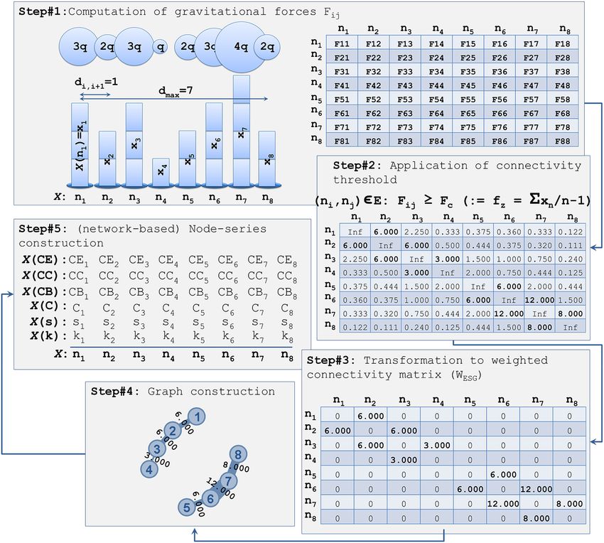
www.nature.com/scientificreports/
(wij > 0) indicate that nodes i,j have homogeneous arithmetic signs, where negative cases (wij < 0) imply that they
have heterogeneous signs. Also, high wij scores may imply either that nodes i,j are close in the time-series line,
in terms of spatial proximity, or that they have relatively high arithmetic values or both. Within the context of
the electrostatic conceptualization, the attraction expressed by a negative Coulomb-like force (wij = –Fij) can be
seen as a tendency of the nodes to balance their heterogeneity and converge toward the horizontal axis, whereas
the repulsion expressed by a positive force (wij = + Fij) can be seen as a tendency of the nodes to escape from
their homonymous electrostatic balance and thus to evolve (either increasingly or decreasingly) through time.
By definition, Coulomb’s law determines a field of infinite distance, where the electrostatic forces are noticed
at infinity, although they are negligible. This property makes the ESG by default a fully connected (complete)
graph Kn, namely a graph where all nodes are linked to any other. Provided that a complete graph Kn has a trivial
topology, in terms of complexity (since the average degree is always k
= n–1 and most of other metrics, such as
average path length, network diameter, graph density, and clustering coefficient are equal to one), we filter the
set E of the ESG connections, aiming to generate more complex topologies
of electrostatic graphs. In particular,
we consider a threshold Fc, defined within the interval Fc ∈ min Fij , max Fij , so that the weighted con-
nectivity matrix WESG include those values that are equal or above Fc, as it is expressed by the relation:
WESG = {Fij �= 0 ∈ F(X) : Fij ≥ Fc } ⊆ F(X), (3)
where F(X) is the Coulomb-like matrix defined in relation (1). This filtering allows considering numerous elec-
trostatic graphs ESG(X), which are expressed as a function WESG = f(Fc) of the threshold-variable Fc. To introduce
a reference value to the threshold-variable Fc, we define a typical value fz by the relation:
√ √
1 n |�x�| · |�x�|
Fc (fz ) = fz = · xn = · �x� = n · sgn(�x�) ·
√
2 , (4)
n−1 n n−1 n−1
where n is the number of time-series nodes, �·� is the average operator, and sgn(·) is the sign (or signum)
function26. In numeric terms, the fz filtering describes that non-zero elements of the weighted ESG’s connectiv-
ity matrix are those with values higher than the adjusted mean-value n−1 n
· �x� of the time-series X. In physical
(electrostatic) terms, fz describes
√ an electrostatic force that is n-times greater than this applied to a pair of particles
√ qi, qj = |�x�|(i.e. equal to the square-root of the absolute mean-value of the time-series
with electrical charges
X), which are dij = n − 1 (i.e. equal to the square-root of the time-series length) steps of separation distant.
Within this context, the proposed ESG algorithm is implemented in four steps, as it is shown in Fig. 2. First,
we compute the matrix F(X) of Coulomb-like forces, according to the relations (1) and (2). Secondly, we apply
to F(X) the connectivity filter and compute the weighted connectivity matrix WESG, according to the relations (3)
and (4). Thirdly, we manage the disconnected data (i.e. mainly the diagonal element yielding infinite computa-
tions due to zero distances included in the denominator) of F(X), by substituting “inf ” (infinite) values by zeros.
Fourthly, we create the graph-layout of the ESG(X) based on the weighted connectivity matrix WESG.
According to the first four steps of the algorithm, we can generate the electrostatic graph ESG(X), which is
associated with a time-series X and is an undirected and weighted graph with a non-trivial topology. In this graph
model, we can further compute several network measures and metrics and thus reveal the topological properties
of the ESG. Therefore, at the fifth and final step of the algorithm, we compute node-series of network measures
of the ESG(X), and afterward, we compare their structural relevance with this of the source time-series X. The
procedure is described in more detail in the following paragraphs.
Node‑series of network measures. The electrostatic graph ESG(X) is a graph-model GESG(V,E) where
each network node vi ∈ V is the same with a time-series node i ∈ X, namely vi≡i ∈ V,X. Therefore, for every node-
measure Y (e.g. node degree, local clustering coefficient, closeness, betweenness, and eigenvector centrality, etc.)
of the ESG, we can arrange the scores Y(vi) = yi into the time-series X = {x1, x2,…, xn} ordering, and thus to
configure node-series X(Y) = {y1, y2,…, yn} of the ESG network measures that are associated with the source
time-series. This allows comparing the source time-series X with these of the ESG node-series X(Ys) and detect-
ing possible structural similarities that can be seen as a measure of relevance between the time-series and the
ESG. The available network (node) measures that participate in the construction of the node-series are shown
in Table 1.
In terms of notation, for a (source) time-series X = {x1, x2,…, xn}, where n∈ N and xi∈ R , we can write its
associated node-series for the network measure Y as X(Y) = {Y(x1), Y(x2),…, Y(xn)} = {y1, y2,…, yn}. We can read
that X(Y) is “the node-series of the network measure Y, which is computed for the ESG that is associated with
the time-series X” or, in brief, that X(Y) is “the node-series of (the measure) Y for the ESG”. Within this context,
we can compute the node-series for the measures of degree X(Y = k) = {k1, k2,…, kn}, strength X(s) = {s1, s2,…,
sn}, clustering coefficient X(C) = {C1, C2,…, Cn}, betweenness centrality X(CB) = {CB1, CB2,…, CBn}, closeness
centrality X(CC) = {CC1, CC2,…, CCn}, and eigenvector centrality X(CE) = {CE1, CE2,…, CEn}, according to the
mathematical formulas shown in Table 1. Provided that we can generate a node-series for any graph G(X) that
is associated with a time-series X, we can include a subscript index in the notation XG(Y) when necessary (e.g.
XESG(k)) to denote the type of graph that the time-series is associated with.
The effect of the connectivity threshold on the ESG topology. The connectivity threshold Fc that is
applied to the Coulomb-like matrix, according to relation (3), is determinative for the configuration of the ESG
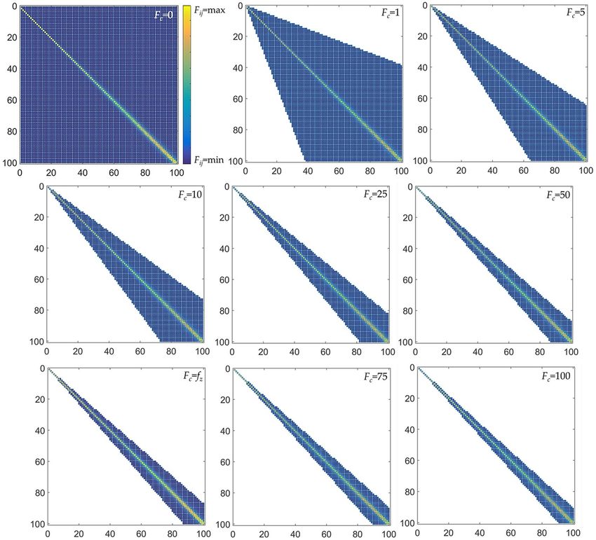
topology. To illustrate this, let us consider the series X1:100 = {1, 2,…, 100} of the first hundred natural numbers.
By applying to this series sequentially the connectivity thresholds Fc = 0, Fc = 1, Fc = 5, Fc = 10, Fc = 25, Fc = 50,
Fc = fz, Fc = 75, and Fc = 100, we get various ESGs, as it is shown in Fig. 3.
Scientific Reports | (2021) 11:11785 | https://doi.org/10.1038/s41598-021-89552-2 3
Vol.:(0123456789)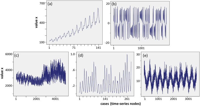
www.nature.com/scientificreports/

                                                  Figure 2.  The methodological framework of the study. Steps #1–#4 describe the ESG algorithm generating an
                                                  electrostatic graph from a time-series X = {xi | i = 1, …, 8}. Step#5 describes the process of generating secondary
                                                  time-series from the network measures of ESG(X).

           Measure                            Description                                                                                                          Mathematical Expression

                                                                                                                                                                   ki = k(i) =   δij , where
                                                                                                                                                                                          j∈V
           Node Degree (k)                    The number of edges being adjacent to a node i
                                                                                                                                                                             1, if eij ∈ E
                                                                                                                                                                    δij =
                                                                                                                                                                            0, otherwise

                                                                                                                                                                   si = s(i) =          δij · wij ,
           Node strength (s)                  The sum of edge weights being adjacent to a given node i                                                                                j∈V (G)

                                                                                                                                                                   where wij = w(eij )

                                              The number of a node’s connected neighbors E(i), divided by the number of the total triplets ki(ki–1) shaped by
           Local Clustering Coefficient (C)                                                                                                                        C(i) =           E(i)
                                              the node i                                                                                                                        ki ·(ki −1)
                                                                                                                                                                                                 n
                                              Total binary distance d(i,j) computed on the shortest paths originating from a given node i and having destination CC(i) =           1
                                                                                                                                                                                           ·

                                                                                                                                                                                                          dij = d i
           Closeness Centrality (CC)
                                              all the other nodes j in the network. This measure expresses the node’s reachability in terms of steps of separation                n−1
                                                                                                                                                                                               j=1,i�=j

           Betweenness Centrality (CB)        Fraction of all shortest paths σ(i) including a given node i, to the number σ of all the shortest paths in the network CB(i) = σ (i) σ


                                              Spectral measure expressing the influence of node i in the network. In the formula N(i) expresses the neigh-
           Eigenvector Centrality (CB)        borhood of node i, aij an element of the adjacency, xj the j-th component of the adjacency’s eigenvector with                       1
                                                                                                                                                                   CE(i) =           ·            aij · xj
                                              eigenvalue equal to λ                                                                                                                       j∈N(i)

                                                  Table 1.  The node measures that are considered in the analysis 1,27-29

                                                     As it can be observed, the ESGs shown in Fig. 3 appear quite different in terms of graph density and node
                                                  arrangement in the adjacency matrix. In particular, as the Fc becomes greater, the connectivity strip toward the
                                                  main diagonal in the adjacency matrix becomes narrower, expressing each time a separate connectivity pattern.
                                                  To examine whether and how the network topology is affected by changes in Fc, we compute a set of network

          Scientific Reports |         (2021) 11:11785 |                     https://doi.org/10.1038/s41598-021-89552-2                                                                                               4

Vol:.(1234567890)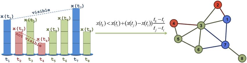
www.nature.com/scientificreports/
Figure 3. Sparsity (spy) plots of the ESGs that are associated with the series X1:100 = {1, 2,…, 100} and are
computed for the connectivity thresholds Fc = 0, Fc = 1, Fc = 5, Fc = 10, Fc = 25, Fc = 50, Fc = fz, Fc = 75, and Fc = 100.
measures and metrics (average degree k
, clustering coefficient C, graph density ρ, modularity Q, average path
length l
, network diameter d(G), and the number of components) for a series of ESGs that are generated
by applying connectivity thresholds ranging within the interval Fc∈[0, n2 = max{ X1:100}2 = 104]. This approach
assumes that the network topology is collectively approximated by the set of available network measures, where
each measure represents a certain topological aspect. The results of the analysis are shown in Fig. 4, where each
network measure is expressed as a function of the connectivity threshold Fc.
Also, is evident that all network measures considerably fluctuate as the connectivity threshold Fc changes.
The cases of average degree k
(Fig. 4a), clustering coefficient C (Fig. 4b), and graph density ρ (Fig. 4c) follow a
declining pattern to the changes of Fc, the cases of average path length l
(Fig. 4e) and graph density d(G) (Fig. 4f)
follow a bell-shaped pattern of negative skew (asymmetry), whereas the number of components (Fig. 4g) follows
an increasing pattern. For the case of modularity Q (Fig. 4d), the performance of this measure appears consider-
ably invariant along the biggest part of the Fc’s interval. As far as the typical value fz is concerned, we can observe
that this value cannot be related to border (i.e. min or max) distribution values, but it can be quite indicative of
the average performance of the topological aspects of the ESGs. This indication can support the goodness of the
choice of defining the typical fz value within a physical (Coulomb-like) context, as it is shown in relation (4).
Overall, this analysis shows that the choice of the connectivity threshold Fc can be determinative to the
topological features and generally the topology of the resulting ESG. This observation is evident even by the
examination of a simple linear series of natural ascending numbers, which can only be considered as an indicative
approach for the ESG construction. However, even this simple consideration sufficed to highlight the dependence
between the connectivity threshold and the ESG’s network topology and thus to introduce a methodological
path for optimally defining the Fc value. The examination of the optimum or most representative threshold is
a matter of specialized optimization analysis that introduces avenues of further research and falls outside the
scope of this paper. However, the physically defined approaches, as this of the Coulomb-like definition of the
Fc shown in relation (4), or others utilizing methods from other disciplines can become insightful toward this
optimization direction and are suggested for further research promoting multidisciplinary conceptualization. For
instance, further research on this topic can apply to different types of time-series and more thorough optimiza-
tion analysis in the choice of Fc. For the scope of this paper, the choice of the typical value fz for the connectivity
Scientific Reports | (2021) 11:11785 | https://doi.org/10.1038/s41598-021-89552-2 5
Vol.:(0123456789)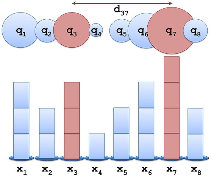
www.nature.com/scientificreports/
Figure 4. . Line diagrams showing how the network measures of (a) average node degree k
, (b) clustering
coefficient C, (c) graph density ρ, (d) modularity Q, (e) average path length l
, (f) network diameter d(G), and
(g) number of components change as a function of the connectivity threshold Fc, for a series X1:100 = {1, 2,…,
100}, where Fcrangeswithin the interval Fc ∈[0, max{ X1:100}2]. The bold vertical line represents the typical value fz
defined at relation (4), whereas the dashed horizontal line a point estimate of the average y values.
threshold is considered satisfactory to provide a reference value that is representative of the average topological
features of the ESGs.
Testing the performance of the ESG algorithm. The analysis examines five different types of time-
series, as it is shown in Fig. 5. The first one (Fig. 5a) was extracted from AirPassengers30 and is a time-series with
a linear trend (abbreviated: Xa≡AIR), including the monthly totals of US airline passengers for the period 1949
to 1960 (144 cases). The second one (Fig. 5b) was extracted from L orentzTS31 and is a typical Lorentz chaotic
time-series (Xb≡CHAOS) generated from the Lorenz differential equations, on standard values sigma = 10.0,
r = 28.0, and b = 8/3. This time-series has a length of 1900 cases. The third one (Fig. 5c) was extracted from
DEOK.hourly32 and is a part (the first 5000 cases) of a broader stationary time-series (of 57,739 cases) including
estimated energy consumption, in Megawatts (MW), for the Duke Energy Ohio/Kentucky (Xc≡DEOK). Next,
Scientific Reports | (2021) 11:11785 | https://doi.org/10.1038/s41598-021-89552-2 6
Vol:.(1234567890)www.nature.com/scientificreports/
Figure 5. The source (reference) time-series considered in the analysis represent distinctive different patterns,
where (a) is an air-passengers time-series with linear trend (Xa: 144 cases, including the monthly totals of a US
airline passengers for the period 1949 to 1960), (b) is the typical Lorentz chaotic time-series (Xb: 1900 cases,
created from the Lorenz equations, on standard values sigma = 10.0, r = 28.0, and b = 8/3), (c) is a part (Xc:
5000 cases) of a broader stationary time-series including estimated energy consumption, in Megawatts (MW),
for the Duke Energy Ohio/Kentucky, (d) is a periodical time-series (Xd: 280 cases, including wolfer sunspot
numbers for the period 1770 to 1771), and (e) is a cyclic time-series (Xe: 3650 cases, including daily minimum
temperatures in Melbourne, Australia, for the period 1981–1990).
the fourth one (Fig. 5d) was extracted from Wolfer-sunspot-numbers33 and is a periodic time-series including
Wolfer sunspot numbers (Xd≡SUNSPOTS), for the period 1770 to 1771 (280 cases). The fifth one (Fig. 5e) was
extracted from Daily-minimum-temperatures-in-me34 and is a cyclical time-series including daily minimum
temperatures in Melbourne, Australia (Xe≡TEMP), for the period 1981–1990 (3650 cases). Links to the time-
series databases are available in the reference list.
To examine the effectiveness of the proposed algorithm, we firstly compare the structure of the source time-
series X with its node-series XESG(Ys) of the ESG node measures (Ys). Such comparisons are driven by the
rationale that the ESG is a transformation (conversion) of a time-series to a complex network and therefore
possible similarities that can be detected in the structural properties (e.g. data variability, linear trend, chaotic,
stationary, periodic, and cyclical structure) between the original time-series and its associated ESG node-series
can be seen as aspects of homeomorphism describing this transformation. In general, this approach is expected
to illustrate the level at which the topology of the associated electrostatic graph ESG(X) sufficiently incorporates
structural information of the source time-series X. Secondly, we compare the structure of the XESG(Ys) node-series
with this of their concordant node-series XVGA(Ys) of the node measures (Ys) computed in the visibility graphs
defined by Lacasa et al.5. The comparisons between the source time-series and its associated node-series (either
of ESG or VGA conversion) build on a multilevel analysis consisting of five tests; the first one detects similarities
in data-variability (i.e. whether the original time-series and the node-series have the same fluctuation patterns)
based on the Pearson’s bivariate coefficient of correlation35,36, the second one in linear-trend by using the Linear
Regression (LSLR) fi tting36, the third one in chaotic-structure based on the correlation dimension and embed-
ding dimension diagram37, the fourth one in stationary-structure based on the augmented Dickey-Fuller test
(ADF) for a unit root 38, and the fifth one in periodic-structure based on autocorrelation f unction38. Each test is
briefly described in the following paragraphs.
The visibility graph algorithm. The natural visibility algorithm (NVG) was proposed by Lacasa et al.5 and
builds on the intuition of considering a time-series as a path of successive mountains of different height, where
each represents the value of the time-series at a certain time. In this time-series landscape, an “observer” stand-
ing on the top of a mountain can see (either forward or backward) as far as possible, provided that no other top
obstructs its visibility field (Fig. 6).
In mathematical terms, each time-series node (ti, x(ti)) corresponds to a graph node i≡(ti, x(ti))∈ V, and thus
two nodes i,j ∈ V are connected (i,j)∈ E in the visibility graph when the following inequality (NVG connectivity
criterion) is satisfied:
tk − ti
X(tk ) < X(ti ) + (X(tj ) − X(ti ))
tj − ti
, ∀k ∈ (i, j), (6)
Scientific Reports | (2021) 11:11785 | https://doi.org/10.1038/s41598-021-89552-2 7
Vol.:(0123456789)www.nature.com/scientificreports/
Figure 6. (left) Example a pair of visible (shown in blue colour) and another of not visible (shown in red
colour) time-series nodes (generally shown in green colour) defined according to the natural visibility algorithm
(NVG), (right) the visibility graph generated from the time-series shown at the left side.
where X(ti) and X(tj) are the numerical values of the time-series nodes (ti, x(ti))≡i and (tj, x(tj))≡j and ti, tj express
their time points. In geometric terms, a visibility line can be drawn between two time-series nodes i,j ∈ V, if no
other intermediating node (tk, x(tk))≡k obstructs their visibility. That is, two time-series nodes are connected in
the visibility graph whether no other intermediary node is higher so that to intersect the visibility line defined
by this pair of nodes (Fig. 6). Therefore, two time-series nodes can enjoy a connection in the associated vis-
ibility graph if they are visible through a visibility line. The visibility algorithm conceptualizes the time-series as
a landscape and generates a visibility graph associated with this landscape. The associated (to the time-series)
visibility graph is a complex network where complex network analysis can be further a pplied8,16.
Correlation analysis. At the first step of the analysis, we detect linear correlations between the source time-
series X and the available (ESG and VGA) node-series. This approach examines whether the original time-series
X and the node-series {Xi(k), Xi(s), Xi(C), Xi(CB), Xi(CC), and Xi(CE) | i = ESG,VGA} have the same fluctuation
patterns and thus they can be considered as relevant in terms of data variability. In this analysis, the Pearson’s
bivariate coefficient of correlation35,36 is used, which ranges at the interval rX,Y ∈[–1,1] and detects linear (either
positive or negative) correlations when |rXY | → 1.
Test of the linear trend. To detect a linear trend, we apply linear fittings to the source time-series X and
to its associated node-series { Xi(k), Xi(s), Xi(C), Xi(CB), Xi(CC), and Xi(CE) | i = ESG,VGA}. According to this
a pproach36, a linear curve ŷ = b · f (x) + c is fitted to the available data that bests describes their variability. The
curve fitting algorithm estimates the parameters b, c minimizing the square differences yi − ŷi36, according to
the relation:
n n
2
2
(7)
min e = yi − ŷi = yi − bi fi (x) + c ,
i=1 i=1
where yi express the observed and ŷi the estimated values. The optimization method that is used is the Least-
n
2
Squares Linear Regression (LSLR) method36, which assumes that the differences e = yi − ŷi follow the
i=1
normal distribution e ~ N(0,σe2). The goodness of the model fit is measured by the coefficient of determination
R2, which is defined by the e xpression35,36:
n
2
n
2
R2 = ŷi − y yi − y , (8)
i=1 i=1
where y is the average of the observations and n is the number of cases (i.e. the series length). The coefficient of
determination expresses the amount of variability of the response variable that is expressed by the linear model
and ranges within the interval [0,1], indicating perfect linear determination when R2 = 135,36. Within this context,
amongst the ESG and VGA node-series, those being closer to the source time-series X in determination and
model configuration (i.e. values in b and c estimators) are considered as more relevant to X in terms of linear
trend.
Detection of chaotic structure. To detect chaotic structure in a time-series, we examine the patterns of
the correlation (v) versus the embedding dimension (m) scatter plots (v,m). According to the Chaos theory37,
the correlation dimension (v) is a measure of the dimensionality of the space occupied by a set of random points
and thus is used to determine the dimension of the fractal objects, which is often called fractal dimension. For a
time-series X = {xi | i = 1, …, n}, the correlation integral C(ε) is calculated by the e xpression39,40:
N(ε)
C(ε) = lim ∼ εv , (9)
n→∞ n2
where N(ε) is the total number of pairs of time-series points (xi, xj) with a distance smaller than ε, namely
d(xi,xj) = dij < ε. As the number of points tends to infinity (n → ∞), and therefore as their corresponding distances
Scientific Reports | (2021) 11:11785 | https://doi.org/10.1038/s41598-021-89552-2 8
Vol:.(1234567890)www.nature.com/scientificreports/
tend to zero (dij → 0), the correlation integral tends to the quantity C(ε) ~ εv, where v is the so-called correlation
dimension. Intuitively, the correlation dimension expresses the ways to which the points can be close to each
other along different dimensions and is expected to rise faster when the space of embedding is of a higher dimen-
sion. Therefore, the correlation (v) versus the embedding dimension (m) diagram (v,m) can provide insights into
how the time-series points are close to each other, as the dimensionality of the space of embedding increases39,40.
Within this context, amongst the ESG and VGA node-series, those with the (v,m) diagram being closer to the
source time-series X are considered as more relevant to the original time-series, in terms of chaotic structure.
Detection of stationarity. To detect stationarity in the available series we apply the augmented Dickey-
Fuller test (ADF) for a unit root 38. The ADF algorithm examines the null hypothesis (Ho) that a unit-root is
present in the model’s time-series data, which is expressed by the relation:
yt = c + δt + φ · yt−1 + β1 · �yt−1 + · · · + βp · �yt−p + εt , (10)
where Δ is the differencing operator (Δyt = yt − yt−1), p is the number of lagged difference terms (specified by the
user), c is a drift term, δ is a deterministic trend coefficient, φ is an autoregressive coefficient, βi are the regression
coefficients of the lag differences, and εt is a mean zero innovation process. According to Eq. (10), the unit-root
hypothesis testing is expressed as f ollows38:
Ho : φ = 1 vs.H1 : φ < 1, (11)
and the (lag adjusted) test statistic DF is defined by the e xpression38:
⌢
N(φ − 1)
DF = ⌢ ⌢
, (12)
(1 − β 1 − ... − β p )
where the uppercase symbol ‘^’ expresses an estimator. Within this context, amongst the node-series of ESG and
VGA, first those satisfying the null hypothesis and then those that have more similar DF statistics with the source
time-series X are considered as more relevant to the original time-series, in terms of stationarity.
Detection of periodicity and cyclical structure. To detect periodicity in the available time-series we
use the autocorrelation function (ACF), which is defined as:
γx (s, t)
ρ(s, t) = √ , (13)
γx (s, s)γx (t, t)
where (s,t) are time points and γx(s,t) is the autocovariance function of the variable x38. In general, the ACF
measures the linear predictability of the series at time t by using only the value xs (at time s) with a time-lag
dt = t − s. The ACF lies within the interval − 1 ≤ ρ(s,t) ≤ 1, where positive coefficient values imply a positive linear
trend and negative values a negative one. Based on the ACF, we construct a set of ACF-variables, where the first
refers to the source time-series X and the others to the node-series Xi(k), Xi(s), Xi(C), Xi(CB), Xi(CC), and Xi(CE),
where index i can be either i = ESG or VGA. Each variable includes 30 elements corresponding to ACFs of lag
dt = 1,2,…,30, respectively, namely:
ACF(X) = {ρ(t, t + 1), ρ(t, t + 2), ..., ρ(t, t + 30)}. (14)
By constructing these ACF-variables, we compute the Pearson’s bivariate coefficient of c orrelation 35,36
to detect
linear correlations between the ACF(X) variable of the source time-series X and the other node-series variables.
Within this context, amongst the available ESG and VGA node-series variables, those being higher correlated
with the source time-series X are considered as more relevant to the original time-series in terms of periodicity
and cyclical (i.e. periodic with a constant oscillation height) structure.
Results
Spy plots and graph layouts. The spy plots and graph layouts of the ESG(X) and VGA(X) graphs associ-
ated with the time-series X are shown in Fig.A1-A5 (in the Appendix). The spy plots are matrix-plots displaying
with dots the non-zero elements of the adjacency matrix and they can thus represent the graph topology within
the matrix-space3,41. On the other hand, network visualization is implemented by using the “Force-Atlas” layout,
which is available in the open-source software of Bastian et al.42. This layout is generated by a force-directed
algorithm, which applies repulsion strengths between network hubs while it arranges hubs’ connections into
surrounding clusters. Graph models that are represented in this layout have therefore their hubs centered and
mutually distant (i.e. intermediate distance between hubs is the highest possible), whereas lower-degree nodes
are placed as closely as possible to their hubs3.
As it can be observed in Fig.A1 (Appendix), the ESG(Xa) spy plot has a connectivity pattern configuring a tie
(along the main diagonal) of increasing width (Fig.A1.a,c, Appendix), which appears indicative of the increasing
trend of the source time-series (Xa = AIR). An aspect of such trend is also evident in the chain-like ESG(Xa) graph
layout (Fig.A1.e, Appendix), where a cluster of hubs appears on the right side that resembles the tie configuration
shaped in the spy plot. Also, the saw-like pattern of the source time-series appears smoother in the pattern of
the 2d ESG(Xa) spy plot (Fig.A1.a, Appendix), whereas is more evident in the diagonal arrangement of the 3d
ESG(Xa) spy plot (Fig.A1.c, Appendix). On the other hand, the VGA(Xa) spy plot configures a periodic pattern
Scientific Reports | (2021) 11:11785 | https://doi.org/10.1038/s41598-021-89552-2 9
Vol.:(0123456789)www.nature.com/scientificreports/
(Fig.A1.b,d, Appendix), where no linear trends are visible. This can be also observed in the VGA(Xa) graph layout
(Fig.A1.f, Appendix), which shapes an almost symmetric hub-and-spoke pattern.
In Fig.A2, the ESG(Xb) spy plot configures a fractal-like tiling (Fig.A2.a, Appendix) illustrating a chaotic
structure. Although such structure in the ESG(Xb) graph layout (Fig.A2.f, Appendix) is not that clear, we can
observe two major components composing the electrostatic graph of Xb (Lorentz time-series). This is a result
of the positive and negative values in the structure of the source time-series (Xb), illustrating the ability of the
electrostatic graph (ESG) algorithm to generate disconnected g raphs1,41,27. Although connectivity is generally
a desirable property in complex networks, the ability of the ESG algorithm to generate disconnected graphs
can be insightful for removing past or unnecessary information (noise) of the time-series, therefore proposing
avenues for further research. On the other hand, the VGA(Xb) graph layout (Fig.A2.f, Appendix) better illustrates
a chaotic structure than its spy plot (Fig.A2.b,d Appendix) does, which is more illustrative to a periodic than to
chaotic structure.
Next, in Fig.A3 (Appendix) the ESG(Xc) spy plot (Fig.A3.a,c, Appendix) configures a tie (along the main
diagonal), with an almost constant width, which complies with the stationary structure of the source time-series
(Xc = DEOK). Some evidence of stationarity can be also observed in the concentrated (solid-like) pattern of the
ESG(Xc) graph layout (Fig.A3.e, Appendix). On the other hand, neither the VGA(Xc) spy plot (Fig.A3.b,d) nor
graph layout (Fig.A3.f, Appendix) are illustrative of a stationary structure describing the original time-series (Xc).
In Fig.A4 (Appendix), the ESG(Xd) spy plot also configures a tie (along the main diagonal) with repeated
knot-concentrations (Fig.A4.a,c, Appendix), which complies with the periodic structure of the source time-series
(Xd = SUNSPOTS). Some insightful indications of such periodicity can be also observed in the clustered (torus-
like) pattern that is shown in the ESG(Xd) graph layout (Fig.A4.e, Appendix). On the other hand, the VGA(Xc)
spy plot (Fig.A4.b,d, Appendix) has an interesting periodic pattern, which is slightly mixed by the square areas
of the other connections. However, the VGA(Xd) graph layout (Fig.A4.f, Appendix) does not appear illustrative
of the periodic structure describing the source time-series (Xd).
Finally, the ESG(Xe) spy plot configures a tie (along the main diagonal) with repeated slightly thicker segments
(Fig.A5.a,c, Appendix), which can relate to the cyclical structure describing the source time-series (Xe = TEMP).
However, such cyclical structure is almost hidden in the chain pattern of graph components that have an odd
arrangement in the ESG(Xd) graph layout (Fig.A5.e, Appendix). Periodicity can become clearer whether the
layout will be further stretched to succeed symmetric arrangement similar to this of Fig.A4.e (Appendix). On
the other hand, the VGA(Xc) spy plot shapes a clearer periodic pattern (Fig.A5.b,d, Appendix), which (although
difficult) can be observed in the graph layout (Fig.A5.f, Appendix). Overall, the proposed ESG algorithm appears
at least as capable as the VGA is in generating graphs of topologies representative of their source time-series.
This observation will be also quantitatively tested in the following sections.
Correlation analysis. To compare patterns in data variability between the source and the ESG and VGA
node-series (see Fig. A6-A10, Appendix), we apply a Pearson’s bivariate correlation analysis, the results of which
are shown in Table 2. Amongst the available correlation coefficients, we compare concordant pairs (r(X,XESG(z),
r(X,XVGA(z)|z = k, C, CB, CC, and CE) between ESG and VGA node-series and we denote pairwise maxima
(max{(r(X,XESG(z), r(X,XVGA(z)}) in bold font. Cases with the XESG(s) node-series are paired with those of cor-
responding degree XVGA(k), due to the similarity of the measures of node degree (k) and node strength (s), for
the binary and weighted networks. Within this context, according to Table 2, in the case of the Xa time-series,
the variability of the ESG node-series is overall closer to this of the source time-series (Xa) than the variability of
the VGA node-series overall is, because the ESG node-series count 5 out of 6 maxima, whereas the VGA node-
series count just one. This observation implies that the ESG transformation generates graphs that better preserve
fluctuations with a linear trend of the original time-series than the VGA does. On the contrary, in the case of
the chaotic time-series (Xb), the VGA node-series count 5 out of 6 maxima (a double count is given for the k,s
pair), whereas the ESG node-series count just one. This observation implies that the VGA transformation better
preserves chaotic fluctuations of the original time-series than the ESG does.
In the case of the Xc (DEOK), the ESG node-series count 4 out of 6 maxima, whereas the VGA node-series
count 2 out of 6, which implies that the ESG transformation better preserves stationary fluctuations of the original
time-series than the ESG does. In the case of the Xd (SUNSPOTS), the ESG node series count 5 out of 6 maxima,
whereas the VGA node-series count just one, which implies that the ESG transformation better preserves peri-
odical fluctuations of the original time-series than the VGA does. In the case of the Xe (TEMP) both the ESG
and the VGA node-series count 3 out of 6 maxima, showing a balanced performance. As far as the measure of
strength (s) (see Fig. A11, Appendix) is concerned, the analysis shows that, for all types of time-series except
the chaotic one (Xb, CHAOS), the ESG node-series have higher performance than the VGAs. Overall, this pair-
wise consideration illustrates that the variability of ESG node-series is closer to the source time-series (Xi) than
of the VGAs, since the first count 18 out of 30 maximum cases, whereas the latter count 12 out of 30 maxima.
Test of the linear trend. The test of the linear trend was applied to ESG and VGA node-series associated
with the Xa (AIR) time-series, which is a time-series with a known linear trend. The results of the analysis are
shown in Table 3, where first it can be observed that the source (Xa: AIR) time-series is well described by a linear
regression model (R2 = 0.8536). However, none of the VGA node-series can sufficiently retain this linear struc-
ture, as is evident by the low coefficients of determination ranging from R2 = 0.0002 to R2 = 0.0132.
On the contrary, the ESG node-series of degree XESG(k), strength XESG(s), and eigenvector centrality XESG(CE)
have a considerable linear structure, as is denoted by their respective coefficients of determination R2 = 0.6916,
R2 = 0.8012, and R2 = 0.7579. It should be noted that among these cases, the strength node-series XESG(s) have the
Scientific Reports | (2021) 11:11785 | https://doi.org/10.1038/s41598-021-89552-2 10
Vol:.(1234567890)www.nature.com/scientificreports/
VariableXij(z(a)) (node-series)
j = VGA j = ESG
VariableXi(source time-series) Measure z=k z=C z = CB z = CC z = CE z=k z = s(b) z=C z = CB z = CC z = CE
r(Xi,Xij(z)) 0.331** -0.158 0.250** -0.232** 0.254** 0.805** 0.981** 0.358** -0.144 -0.359** 0.837**
i = a (AIR) sig.(c) 0.000 0.059 0.002 0.005 0.002 0.000 0.000 0.000 0.085 0.000 0.000
n(d) 144
r(Xi,Xij(z)) 0.516** 0.019 0.188** -0.185** 0.201** -0.008 0.002 -0.022 0.020 0.103** -0.132**
i = b (CHAOS) sig 0.000 0.401 0.000 0.000 0.000 0.712 0.919 0.345 0.375 0.000 0.000
n 1900
r(Xi,Xij(z)) 0.354** -0.570** 0.148** -0.140** 0.157** 0.890** 0.989** -0.549** 0.179** 0.088** 0.725**
i=c
sig 0.000 0.000 0.000 0.000 0.000 0.000 0.000 0.000 0.000 0.000 0.000
(DEOK)
n 5000
r(Xi,Xij(z)) 0.496** -0.666** 0.478** -0.567** 0.309** 0.768** 0.773** .b 0.593** 0.712** 0.733**
i = d (SUNSPOTS) sig 0.000 0.000 0.000 0.000 0.000 0.000 0.000 0.000 0.000 0.000
n 280
r(Xi,Xij(z)) 0.437** -0.439** 0.211** -0.520** 0.164** 0.908** 0.944** 0.405** 0.123** -0.133** 0.752**
i=e
sig 0.000 0.000 0.000 0.000 0.000 0.000 0.000 0.000 0.000 0.000 0.000
(TEMP)
n 3650
Table 2. Results of the Pearson’s bivariate correlation analysis. a k = node degree, C = clustering coefficient,
CC = closeness centrality, CB = betweenness centrality, CE = eigenvector centrality. c. In pairwise consideration,
XESG(s) is paired with the XVGA(k). c. 2-tailed significance. d. Number of cases. **Correlation is significant at
the 0.01 level (2-tailed). Cases shown in bold indicate maximum coefficients (in absolute terms) between
concordant ESG versus VGA pairs, max{r(X,XESG(z), r(X,XVGA(z)}. Underlined cases indicate max coefficients
(in absolute terms) within each row (for each time-series type).
highest determination. Overall, this analysis illustrates that the ESG algorithm appears more capable than the
VGA in generating graphs that can preserve aspects of the linear trend of the source time-series.
Detection of chaotic structure. In this part of the analysis, the correlation versus the embedding dimen-
sion diagrams (v,m) of the VGA and the ESGs node-series are compared for preserving the chaotic structure of
the source time-series Xb (CHAOS), which is already known as a chaotic time-series constructed on the Lorenz
equations. The results are shown in Fig. A7 (Appendix), where all (v,m) diagrams of the ESG node-series (except
this of eigenvector centrality Xb,ESG(CE)) illustrate the chaotic structure, but of different characteristics than the
source chaotic time-series Xb. However, the (v,m) diagrams of strength Xb,ESG(s) and the original time-series Xb
almost coincide, a fact that implies a relevant chaotic structure between these time-series. On the other hand,
the degree Xb,VGA(k), and possibly the eigenvector centrality Xb,VGA(CE) VGA node-series illustrate a chaotic
structure of high dimensionality, which are also of different characteristics than the original chaotic time-series
Xb. Overall, the chaos analysis shows that the ESG is a more capable transformation in incorporating the chaotic
structure of the source time-series in the network topology. Particularly, the measure of strength shows the most
relevant chaotic structure that almost coincides with this of source time-series.
Detection of stationarity. The test of stationarity was applied to the Xc (DEOK) time-series, which is a
part of an already known stationary time-series. The results of the analysis are shown in Table 4, where, first, it
can be observed that is 7.03% likely for Xc to have a unit-root and thus to be a non-stationary time-series. This
result implies that the null-hypothesis (stating a null unit-root) cannot be rejected, and thus that the source (Xc)
time-series cannot be considered as a stationary one. As it can be observed, the results for all VGA node-series
imply that all cases are statistically safe to be considered as stationary series, which opposes the indication of the
original time-series.
On the other hand, the ESG results imply that 4 out of 5 ESG node-series cannot be considered as stationary
ones and thus resembling the structure of the original time-series. An interesting observation here is that the
p-values of the VGA node-series are (although insufficient indications to retain the null hypothesis) closer than
those of the ESG node-series, in terms of distance. These results imply that the non-stationary effects, which
are immanent in the source time-series, probably appear more intensely in the structure of the ESG node-series
than of the VGA ones.
Detection of periodicity and cyclical structure. This part of analysis builds on bivariate correlations,
which are applied to autocorrelation variables ACF(X) that are defined in relation (14) with lag 1,2,…,30, where
X = Xd (SUNSPOTS time-series), Xe (TEMP time-series), k (degree node-series), C (clustering coefficient node-
series), CB (betweenness centrality node-series), CC (closeness centrality node-series), and CE (eigenvector
centrality node-series). The results of the analysis are shown in Table 5, where the correlation coefficients rXY
and their significances are provided, with X∈{ ACF(Xd), ACF(Xe)} and Y∈{ACFi(k), ACFi(s), ACFi(C), ACFi(CB),
ACFi(CC), ACFi(CE) | where i = VGA, ESG}.
Scientific Reports | (2021) 11:11785 | https://doi.org/10.1038/s41598-021-89552-2 11
Vol.:(0123456789)www.nature.com/scientificreports/
Linear regression
Time-series/
Measure Mathematical expression Determination
xa (AIR) y = 2.6572x + 87.653 R2 = 0.8536
k(xa) y = 0.0118x + 7.0629 R2 = 0.0096
C(xa) y = 0.0006x + 0.7174 R2 = 0.0132
VGAs CB(xa) y = 0.174x + 141.63 R2 = 0.0003
CC(xa) y = -0.0002x + 3.1682 R2 = 0.0002
CE(xa) y = 0.0001x + 0.2013 R2 = 0.0009
k(xa) y = 0.2149x + 13.656 R2 = 0.6916
s(xa) y = 4813.4x – 62,583 R2 = 0.8012
C(xa) y = 0.0009x + 0.6969 R2 = 0.1985
ESGs
CB(xa) y = -1.5134x + 315.61 R2 = 0.0663
CC(xa) y = -0.0106x + 4.6484 R2 = 0.2034
CE y = 0.0069x—0.1143 R2 = 0.7579
Table 3. Linear regression fittings for the Xa (Air) time-series. Cases shown in bold indicate high (> 0.65)
coefficients of determination. Underlined cases highlight the max coefficient, in total.
ADF test
h(a) p-Value DFt (stat) cValue
xc (DEOK) 0 0.0703 -1.7876 -1.9416
k 1 0.0010(b) -16.8555
C 1 0.0010 -8.8160
VGAs CB 1 0.0010 -63.9394 -1.9416
CC 1 0.0176 -2.3683
CE 1 0.0010 -28.4443
k 0 0.2176 -1.1860
s 0 0.3876 -0.7177
C 0 0.3458 -0.8359
ESGs -1.9416
CB 1 0.0010 -20.2674
CC 0 0.1739 -1.3179
CE 0 0.2251 -1.1656
Table 4. ADF test for stationarity of the Xc (DEOK) time-series. a h = 0 indicates failure to reject the unit-root
null (indication: non-stationary series). h = 1 indicates rejection of the unit-root null in favor of the alternative
model (indication: stationary series). b. Cases shown in bold are the closest between concordant measures to
the source time-series scores.
For the case of Xd (SUNSPOTS) time-series, we can observe that 4 out of 6 VGA node-series (k, k≡s, C, CE)
and 3 out of 6 ESG node-series (k, s, CC) are significantly correlated with the original time series Xd. Amongst
these significant results, the VGA node-series have 2 maxima of concordant pairs, whereas the ESG node-series
have also 2 maxima. Moreover, the node-series of strength (Xd,ESG(s)) has the highest correlation coefficient
amongst all available node-series for the SUNSPOTS (Xd) typology, illustrating a better performance of the ESG
algorithm to preserve periodicity, probably due to its capability in generating weighted electrostatic networks.
For the case of Xe (TEMP) time-series, 1 VGA node-series (closeness centrality) is significantly correlated with
the source time-series, where all ESG node-series are significantly correlated with the original time-series. In
terms of pairwise comparisons, the VGA node-series count 1 (out of 6) maximum case, whereas the ESG node-
series count 5 out of 6 maxima. However, although is high, the strength does suggest the highest of the maxima
of the TEMP (Xe) time-series concordant pairs. Overall, this analysis shows that the ESG node-series appear
more capable than the VGA ones in preserving periodic and cyclical characteristics of the source time-series.
Conclusions
This paper proposed a new algorithm, the Electrostatic Graph Algorithm (ESG), for converting a time-series
into a graph (complex network). The ESG builds on the conceptualization of considering a time-series as a series
of stationary and electrically charged particles, on which Coulomb-like forces can be computed. The proposed
algorithm provides an added value to complex network analysis of time-series due to its ability to produce
weighted graphs, which is currently not applicable. This additional property was quantitatively examined in this
paper and was found to produce graphs that are more representative of the structure of the source (original)
time-series, implying that the proposed algorithm suggests a transformation that is more natural rather than
Scientific Reports | (2021) 11:11785 | https://doi.org/10.1038/s41598-021-89552-2 12
Vol:.(1234567890)www.nature.com/scientificreports/
X-variable
ACF(Xd) [SUNSPOTS] ACF(Xe) [TEMP]
Y-variable rXY Sig rXY Sig
ACF(k) 0.8397 0 -0.0803 0.613
ACF(C) 0.7953 0 -0.1311 0.408
VGA ACF(CB) -0.082 0.6057 0.2807 0.0717
ACF(CC) 0.4225 0.0053 1 0
ACF(CE) 0.823 0 0.3306 0.0325
ACF(k) 0.6513 0 0.9999 0
ACF(s) 0.9379 0 0.9196 0
ACF(C) NaN** NaN 0.9999 0
ESG
ACF(CB) 0.2398 0.1261 0.9998 0
ACF(CC) 0.7105 0 0.9999 0
ACF(CE) 0.5601 0.0001 0.9999 0
Table 5. Correlations of ACFs(*) between the source and the node-series (Sunspots and Temp). *ACFs are
computed on lags from 1:30 (relation 13). **Not a number (unable to compute due to zero entries). Cases
shown in bold indicate max coefficients (in absolute terms) according to pairwise (ESG vs. VGA) comparisons
(only statistically significant cases are shown). Underlined cases indicate max coefficients (in absolute terms)
within each column (for each time-series type).
algebraic, in comparison with the existing methods. In particular, the analysis showed that the ESG node-series
can better preserve the linear trend and stationary structural properties of the source time-series in comparison
with the VGA node-series and that they appear slightly better in preserving periodical and cyclical structural
properties of the original time-series than the VGA node-series can. On the other hand, the VGA node-series
appeared slightly better in preserving the chaotic structural properties of the original time-series in comparison
with the ESG node-series, which complies with the claim of the VGA authors regarding the added value of their
algorithm. However, in almost all the parts of the analysis, the ESG node-series of the measure of strength out-
performed their concordant VGA node-series. This result highlighted the added value of the proposed algorithm
in generating weighted graphs, in which the measure of node strength can only be computed. Therefore the ESG
algorithm attributes to the generated graphs information that is more representative of the source time-series,
due to the weights included in the graph structure. Another property of the proposed ESG algorithm to generate
disconnected graphs was indirectly examined by the detection of chaotic and periodic structures, where the ESG
algorithm sufficed to provide disconnected graphs, whereas the VGA did not. This analysis showed that insuf-
ficient connectivity does not restrict the ESG node-series to preserve the structural characteristics of the source
time-series, since the generated electrostatic graphs were representative of the structure of the original time-
series. The authors believe that the property of insufficient connectivity introduces avenues of further research
in the field of noise reduction in the time-series analysis. Other avenues of further research can emerge towards
the direction of either choosing the optimum or most representative connectivity threshold to produce the ESGs
or examining the applicability of the proposed algorithm to solve problems where standard methods fail to ana-
lyze efficiently the time-series, such as the time evolution of stock price, within the framework of Black Scholes
model, and others. The overall approach also suggests a methodological framework for evaluating the structural
relevance between the source time-series and their associated graphs produced by any possible transformation.
Received: 8 December 2020; Accepted: 19 April 2021
References
1. Barabasi, A.-L. Network science. Philos. Trans. R. Soc. Lond. A Math. Phys. Eng. Sci. 371(1987), 20120375 (2013).
2. Brandes, U., Robins, G., McCranie, A. & Wasserman, S. What is network science?. Netw. Sci. 1, 1–15 (2013).
3. Tsiotas, D. Detecting different topologies immanent in scale-free networks with the same degree distribution. Proc. Natl. Acad.
Sci. U. S. A. (PNAS) 116(14), 6701–6706 (2019).
4. Gao, Z.-K., Small, M. & Kurths, J. Complex network analysis of time-series. Europhys. Lett. 116, 50001 (2016).
5. Lacasa, L., Luque, B., Ballesteros, F., Luque, J. & Nuno, J. C. From time-series to complex networks: The visibility graph. Proc. Natl.
Acad. Sci. 105(13), 4972–4975 (2008).
6. Yang, Y. & Yang, H. Complex node-series analysis. Phys. A 387(5), 1381–1386 (2008).
7. Zhang, J. & Small, M. Complex network from pseudoperiodic time-series: Topology versus dynamics. Phys. Rev. Lett. 96(23),
238701 (2006).
8. Tsiotas, D. & Charakopoulos, A. VisExpA: Visibility expansion algorithm in the topology of complex networks. SoftwareX 11,
100379 (2020).
9. Xu, X., Zhang, J. & Small, M. Superfamily phenomena and motifs of networks induced from time-series. Proc. Natl. Acad. Sci.
105(50), 19601–19605 (2008).
10. Gao, Z.-K. & Zin, N. Flow-pattern identification and nonlinear dynamics of gas-liquid two-phase flow in complex networks. Phys.
Rev. E 79(6), 066303 (2009).
Scientific Reports | (2021) 11:11785 | https://doi.org/10.1038/s41598-021-89552-2 13
Vol.:(0123456789)You can also read