Marginally stable phases in mean-field structural glasses - Laboratoire Charles Coulomb
←
→
Page content transcription
If your browser does not render page correctly, please read the page content below
PHYSICAL REVIEW E 99, 012107 (2019)

                              Marginally stable phases in mean-field structural glasses
                                   Camille Scalliet,1 Ludovic Berthier,1 and Francesco Zamponi2
                       1
                      Laboratoire Charles Coulomb, Université de Montpellier, CNRS, 34095 Montpellier, France
                        2
                       Laboratoire de Physique Théorique, Département de Physique, École Normale Supérieure,
                 PSL Research University, Sorbonne Universités, UPMC Université Paris 06, CNRS, 75005 Paris, France

                                             (Received 19 October 2018; published 4 January 2019)

                 A novel form of amorphous matter characterized by marginal stability was recently discovered in the
              mean-field theory of structural glasses. Using this approach, we provide complete phase diagrams delimiting
              the location of the marginally stable glass phase for a large variety of pair interactions and physical conditions,
              extensively exploring physical regimes relevant to granular matter, foams, emulsions, hard and soft colloids,
              and molecular glasses. We find that all types of glasses may become marginally stable, but the extent of the
              marginally stable phase highly depends on the preparation protocol. Our results suggest that marginal phases
              should be observable for colloidal and non-Brownian particles near jamming and for poorly annealed glasses.
              For well-annealed glasses, two distinct marginal phases are predicted. Our study unifies previous results on
              marginal stability in mean-field models and will be useful to guide numerical simulations and experiments aimed
              at detecting marginal stability in finite-dimensional amorphous materials.

              DOI: 10.1103/PhysRevE.99.012107

                      I. INTRODUCTION                                     phase has similar properties across a broad range of physical
                                                                          conditions. In fact, while ordinary glasses formed by cooling
    Twenty years ago, a unified phase diagram for amorphous
                                                                          dense liquids behave roughly as crystalline solids with a high
matter [1] motivated the search for similarities and differences
                                                                          density of defects [13,14], glasses formed by compressing
between the properties of a broad range of materials, from
                                                                          granular materials or non-Brownian emulsions across their
granular materials to molecular glasses [2]. It is now well
                                                                          jamming transition display unique properties distinct from
established that in the presence of thermal fluctuations, dense
                                                                          ordinary solids [5,6]. For example, they may respond to weak
assemblies of atoms, molecules, polymers, and colloidal par-
                                                                          stresses with very large deformations and their low-frequency
ticles undergo a glass transition [3,4] as the temperature is
                                                                          excitations are very different from phonons [15–17]. These
decreased or the density increased. In the absence of thermal
                                                                          properties were theoretically explained by invoking marginal
fluctuations, solidity instead emerges by compressing parti-
                                                                          stability [18,19]: Because these glasses are formed by zero-
cles across the jamming transition [5,6], relevant for foams,
                                                                          temperature compression across a rigidity transition, they
non-Brownian emulsions, and granular materials. These two
                                                                          have barely enough contacts to be mechanically stable. From
transitions have qualitatively distinct features.
                                                                          this observation, several anomalous properties of athermal
    Models of soft repulsive spheres faithfully capture this
                                                                          glasses in the vicinity of jamming can be understood [20].
diversity [7,8], as shown in Fig. 1. The relevant adimensional
                                                                              Theoretical calculations in the framework of the mean-
control parameters are the packing fraction ϕ and the ratio               field theory of the glass transition [11,21–24] have confirmed
of thermal agitation kB T to the interaction strength between             these ideas and suggested in addition the existence of two
particles . A dense assembly of soft particles transforms                distinct types of amorphous solids separated by a sharp phase
into a glass when thermal fluctuations decrease. Glasses can              transition [25,26]. One phase is the normal glass, which
also be obtained by compression at constant temperature, and              corresponds to a free-energy basin that responds essentially
in particular the limit  → ∞ at constant T corresponds to                elastically to perturbations, as any regular solid. The second
compression of colloidal hard spheres. At high density and                is a Gardner glass [27,28]. The Gardner glass is marginally
temperature, the particles constantly overlap and the system              stable due to full replica symmetry breaking, as in mean-
behaves identically to glass-forming liquids. Intermediate                field spin glasses [29]. Physically, marginal stability implies
densities and temperatures describe the glass transition of soft          the existence of long-range correlations in the vibrational
colloids. Jamming transitions are observed in the athermal                dynamics [30,31], an excess of low-frequency modes [32,33],
regime kB T / → 0 relevant for granular materials, foams,                unusual rheological properties [34–36], and system-spanning
and non-Brownian emulsions. Because this occurs deep inside               responses to weak, localized perturbations, manifested, for
the glassy phase at T = 0, jamming transitions are protocol               instance, by diverging mechanical susceptibilities [34,37,38].
dependent and occur over a continuous range of packing                    The Gardner phase may thus provide an elegant route to
fractions ϕJ [9–12].                                                      understand the nature of a multitude of experimental ob-
    The phase diagram in Fig. 1 organizes the physics of                  servations of glassy excitations [25,26]. Explicit mean-field
a broad variety of materials by describing how fluids lose                calculations for the location of marginally stable glasses were
their ability to flow, but incorrectly suggests that the solid            carried out for hard [25,26] and soft [34,39,40] potentials,

2470-0045/2019/99(1)/012107(11)                                   012107-1                                  ©2019 American Physical Society
SCALLIET, BERTHIER, AND ZAMPONI PHYSICAL REVIEW E 99, 012107 (2019)
Dense liquids
two distinct Gardner phases are predicted. Our study extends
and unifies previous analytical studies [26,39,40] and will
serve as a useful theoretical guide for systematic investiga-
tions of marginal stability in finite-dimensional glasses, via
Soft colloids numerical simulations or experiments. In particular, we are
conducting a three-dimensional numerical study that parallels
the calculations presented here [49].
The article is organized as follows. In Sec. II we introduce
Hard
colloids
the models studied in this work. In Sec. III we present the
Grains Emulsions theoretical methods we use. In Sec. IV we present the results
ϕ
for the phase diagrams obtained for a variety of physical
conditions. In Sec. V we discuss our results and provide some
FIG. 1. Schematic (temperature and packing fraction) phase di- perspectives.
agram for soft repulsive spheres and its experimental relevance.
The dynamic glass transition is represented by the red line. Jam-
ming transitions are observed in the athermal limit over a protocol- II. MODELS FOR GLASSY MATERIALS
dependent range of packing fractions (gray line). Different regions of While we are ultimately interested in the phase diagram
the phase diagram are relevant for a variety of amorphous materials, of dense particle systems for which the spatial dimension
indicated in boxes. In this work, we explore in which conditions these is d = 2 or d = 3, we focus on assemblies of particles em-
amorphous materials become marginally stable. bedded in an abstract, but analytically tractable, space of
d → ∞ dimensions. In this limit, an exact solution for the
providing some insight into mean-field phase diagrams. Fur- thermodynamic properties of the liquid and glass phases can
thermore, a way to take into account fluctuations around the be obtained [21,26].
mean-field limit, within the nucleation theory associated with We study several conventional interaction potentials for
the random first-order transition approach, has been proposed glass-forming materials that allow us to interpolate between
in [41]. the various physically relevant limits shown in Fig. 1. In
Numerical simulations and experiments in finite- particular, it is useful to consider the harmonic sphere model
dimensional systems were performed to explore these
r 2
theoretical ideas, yielding contrasting results. Numerical stud- vharm (r ) = 1− θ (σ − r ), (1)
ies of three-dimensional hard-sphere glasses [30,36,42,43] 2 σ
and numerical and experimental study of two-dimensional where r is the interparticle distance, σ the diameter of parti-
hard disks [30,44,45] have revealed a rich vibrational dy- cles, the repulsion strength, and θ (r ) the Heaviside function.
namics, with diverging length scales, suggestive of a Gardner The harmonic sphere model was first introduced to study the
phase. On the other hand, numerically cooling soft glass jamming transition [50] and later studied extensively at finite
formers has only revealed sparse, localized defects [40,46], temperature [7]. Harmonic spheres become equivalent to hard
whereas experimental studies remain inconclusive [47]. It has spheres when → ∞.
also been suggested that in low dimensions localized defects To study the high-density limit relevant for dense liquids,
could induce an apparent Gardner-like phenomenology, harmonic spheres are not useful, as their extreme softness
without an underlying sharp phase transition [40,48]. Overall, gives rise to exotic phenomena that we do not wish to dis-
this recent flurry of results suggests that distinct glassy cuss here. Instead, it is more relevant to analyze the Weeks-
materials may have distinct properties, depending on both Chandler-Andersen (WCA) potential
their preparation and location in the phase diagram of Fig. 1, 4d 2d
thus calling for a systematic microscopic investigation of σ σ
vWCA (r ) = 1 + −2 θ (σ − r ) (2)
marginally stable glassy phases. This is the central goal of the r r
present work.
We use a microscopic mean-field theory to study thermal because it resembles the harmonic potential around the cutoff
soft repulsive spheres in the limit of infinite spatial dimen- r ∼ σ , but behaves as a Lennard-Jones potential at smaller in-
sions to systematically investigate the physical properties and terparticle distance. Our analysis shows that the WCA model
marginal stability of glasses prepared in a wide range of yields results qualitatively similar to the harmonic model at
physical conditions, covering all regimes illustrated in Fig. 1. moderate densities and behaves as the inverse power law (IPL)
For a glass prepared at any given location in Fig. 1, we in- potential
vestigate how its properties evolve under further compression vIPL (r ) = (σ/r )4d (3)
and cooling, thus providing complete phase diagrams locating
simple and marginally stable glasses. We find that all glasses in the high-density limit. Therefore, we decided to concentrate
may become marginally stable, but Gardner phases are more on the two models in Eqs. (1) and (3) to report our results.
easily accessible for systems close to jamming (such as grains, Technically, the harmonic potential is easier to handle, as one
foams, and hard and soft colloids) and for poorly annealed can go one step further analytically than for the WCA model,
glasses obtained by a fast quench. The extent of the marginally which simplifies the numerical resolution of the equations
stable phase depends, in all cases, on the preparation protocol. presented below. The WCA model, on the other hand, is
For well-annealed glasses at intermediate packing fractions, numerically very convenient for finite-dimensional studies,
012107-2MARGINALLY STABLE PHASES IN MEAN-FIELD … PHYSICAL REVIEW E 99, 012107 (2019)
which justifies our effort to study it as well. While the expres- devised to follow glasses created below the dynamical tran-
sion of the harmonic potential is the same regardless of spatial sition [34,57].
dimension, we have extended the standard definitions of the Let us consider an equilibrium configuration Y , extracted
WCA and IPL models in d = 3 to arbitrary dimension d. This from the Boltzmann distribution at (Tg , ϕ̂g ), which falls into
is done because thermodynamic stability and the existence of the dynamically arrested region Tg < Td (ϕ̂g ). To construct the
the thermodynamic limit, a prerequisite for performing the thermodynamics restricted to the glass state Y , we consider
theoretical development described below, require the potential a subregion of phase space probed by configurations X con-
to decay faster than r −d in dimension d [51]. strained to remain close to Y . The configuration X can be at
We consider the thermodynamic limit for N particles in a a different state point (T , ϕ̂), but its mean-square distance to
volume V , both going to infinity at fixed number density ρ = Y is set to a finite value (X, Y ) = r . The free energy fY
N/V . When d = ∞, we can consider monodisperse particles, of the glass state selected by Y and brought to (T , ϕ̂) can be
as crystallization is no longer the worrying issue it is in fi- expressed in terms of a restricted configuration integral [57]
nite dimensions [52,53]. Our adimensional control parameters
are the packing fraction ϕ = N Vd (σ/2)d /V , defined as the Z[T , ϕ̂|Y, r ] = dX e−βV [X] δ(r − (X, Y )),
fraction of volume covered by particles of diameter σ (Vd is (5)
the volume of a d-dimensional unit sphere), and the scaled T
fY (T , ϕ̂|Y, r ) = − ln Z[T , ϕ̂|Y, r ],
temperature T / (in the following, we will set kB = 1). To N
obtain a nontrivial phase diagram in the limit d → ∞, the
where V (X) is the total potential energy of the glass X. The
packing fraction has to be rescaled as ϕ̂ = 2d ϕ/d. Note that in
glass free energy fY in Eq. (5) depends explicitly on the initial
the case of the IPL model, the form of the interaction potential
glass Y . In the thermodynamic limit, its typical value fg is
leads to a unique control parameter = ϕ̂/T 1/4 . We also
given by averaging over all equilibrium states Y ,
define rescaled gaps between particles h = d(r/σ − 1) and
rescaled potentials v̄(h) such that limd→∞ v(r ) = v̄(h): T dY
fg (T , ϕ̂|Tg , ϕ̂g , r ) = − e−βg V [Y ]
N Z[Tg , ϕ̂g ]
v̄harm (h) = h2 θ (−h), v̄IPL (h) = e−4h . (4)
2 × ln Z[T , ϕ̂|Y, r ], (6)
We will be particularly interested in mean-square displace-
ment (MSD) between configurations. In finite where Z[Tg , ϕ̂g ] is the standard configurational integral at
dimensions, (Tg , ϕ̂g ). The free energy has to be computed for the parameter
they are usually defined as D(X, Y ) = N1 i |x i − yi |2 ,
where X and Y represent two configurations. Finite values r verifying ∂r fg = 0 [57]. Note that the density depen-
for the MSD in infinite dimensions are obtained by defining dence of the free energy is encoded by the interaction length
(X, Y ) = d 2 D(X, Y )/σ 2 . scale σ of the potential, which can be changed to induce a
In the following section we summarize the formalism that change in packing fraction.
allows us to compute the thermodynamic properties and the Performing the disorder average in Eq. (6) is challenging.
phase diagram for the above models. Translational invariance, necessary to use saddle-point and
perturbative methods, is broken by the presence of disorder.
To compute the glass free energy in Eq. (6) we use the replica
III. THEORETICAL METHODS method and introduce s + 1 identical replicas of the original
The general strategy of our work is devised to mimic the atomic system to undertake the computation [26,54,57]. The
following experimental protocol. During the gradual cooling master replica represents the initial glass at (Tg , ϕ̂g ), while
or compression of a glass-forming liquid, the equilibrium the s other slave replicas represent the glass at (T , ϕ̂). The
relaxation time τα of the system increases very sharply. For glass free energy can then be expressed in terms of the MSD
a given protocol, there comes a moment where the system between the different replicas. The MSD between any slave
falls out of equilibrium; this represents the experimental glass replica and the master replica are parametrized by r . We
transition, at state point (Tg , ϕ̂g ). After this moment, the make the simplest assumption, called replica symmetric, and
system follows a “restricted” equilibrium, where the amor- consider that all slave replicas are equivalent [57] at a distance
phous structure frozen at the glass transition is adiabatically from each other. At the end of the computation, we take the
followed at different temperature and density, (T , ϕ̂). Our analytic continuation s → 0 and obtain the replica symmetric
analytical strategy follows this protocol closely. We draw an glass free energy
equilibrium but dynamically arrested configuration at (Tg , ϕ̂g ) ∞
2 2r
and follow its thermodynamics when brought adiabatically to − βfg = + ln(π /d 2 ) + ϕ̂g dh P (h)f (h), (7)
d −∞
another state point (T , ϕ̂) within the same glass basin.
defining for simplicity η = ln(ϕ̂/ϕ̂g ),
A. Glass free energy ∞
e−(y−h−/2) /2
2
The state-following protocol described above is possible q(, β; h) = dy e−β v̄(y) √ , (8)
−∞ 2π
if the relaxation time of the initial state is extremely long
[26,54–57]. In infinite dimensions, the equilibrium relax- and
ation time diverges at the dynamic glass transition Td (ϕ̂),
which is of the mode-coupling type [26,58,59]. Our construc- P (h) = eh q(2r − , βg ; h),
tion, which is briefly summarized in the following, is thus f (h) = ln q(, β; h − η). (9)
012107-3SCALLIET, BERTHIER, AND ZAMPONI PHYSICAL REVIEW E 99, 012107 (2019)
Compressing and decompressing a glass corresponds to 101
η > 0 and η < 0, respectively. The glass free energy should Td
be computed with the thermodynamic values for and r , TJ
determined by setting to zero the derivatives of fg with respect 100
to these parameters, which provides two implicit equations for
and r : g3
∞ 10−1 g4
T
∂ g2
2r = + ϕ̂g 2
dh [P (h)f (h)],
−∞ ∂
∞ 10−2 g1
2 ∂
= − ϕ̂g dh f (h) P (h). (10)
−∞ ∂r
10−3
4 10 13 50
B. Dynamic glass transition ϕ
Our method focuses on glasses prepared at (Tg , ϕ̂g ), below
the dynamical transition. Our first task is thus to compute the FIG. 2. Equilibrium mean-field phase diagram for harmonic
dynamical transition line Td = Td (ϕ̂) for the models presented spheres. The dynamical transition Td (red line) separates liquids
that flow (above) from dynamically arrested ones (below). We select
in Sec. II. To do so, let us consider the special case (Tg , ϕ̂g ) =
equilibrium glasses in the dynamically arrested region, for example,
(T , ϕ̂) in the above construction. In that case, = r ≡ g
g1 , . . . , g4 , and follow each glass adiabatically in temperature and
is a solution of fg in Eq. (10) if the glass MSD g verifies
packing fraction. The corresponding state-following phase diagrams
∞ are presented Figs. 5(a)–5(d). Glasses equilibrated above the line TJ
1 ∂q(g , β; h)
= −g dh eh ln q(g , β; h) (dashed line) are jammed once minimized to T = 0, while glasses
ϕ̂ −∞ ∂g
selected below the line are unjammed at T = 0. The state-following
≡ Fβ (g ). (11) phase diagrams of glasses prepared at ϕ̂g = 13 (vertical dashed line)
are presented in Figs. 3 and 4.
For the models considered here, the function Fβ () is pos-
itive, vanishes for both → 0 and → ∞, and has an
The energy is to be computed using the thermodynamic values
absolute maximum in between. This means that Eq. (11) has
for and r , which solve Eqs. (10).
a solution at temperature 1/β only if 1/ϕ̂ is smaller than
We employ the following strategy to numerically solve the
or equal to the maximum of Fβ with respect to . Glassy
equations, find the values of and r at each state point,
states at T thus exist only at packing fractions higher than ϕ̂d ,
and consequently compute the glass potential energy. First, we
defined by
compute the MSD g of the glass at (Tg , ϕ̂g ) by numerically
1/ϕ̂d = max Fβ (). (12) solving Eq. (11). Starting at (Tg , ϕ̂g ) with the initial condition
= r = g , we gradually change the temperature and/or
We numerically solve Eq. (12) for all temperatures and find packing fraction by small steps towards (T , ϕ̂). At the begin-
the dynamical transition line ϕ̂d (T ), or equivalently Td (ϕ̂). ning of each step, we use the values and r of the previous
The result is represented for the harmonic potential in Fig. 2. step as initial guesses. We then solve iteratively Eqs. (10) by
The line separates liquids that flow from dynamically arrested computing the right-hand side of the equations to obtain new
ones. The qualitative behavior of Td (ϕ̂) in the WCA model estimates of and r until convergence is reached. We repeat
is similar to that of harmonic spheres presented in Fig. 2. this procedure until the final state (T , ϕ̂) is reached.
In both cases, the dynamical transition temperature is an
increasing function of ϕ̂ and is defined for ϕ̂ > 4.8067, which D. Gardner transition
corresponds to the dynamical transition for hard spheres [11]. The glass free energy fg defined in Eq. (7) is derived
In the high-density limit, the WCA model behaves as the assuming that the symmetry under permutations of replicas
inverse power law potential and the dynamical transition remains unbroken. At each state point, we must check the
scales as Td ∼ ϕ̂ 4 . The coefficient of proportionality is 1/d4 , validity of this assumption. In practice, we check that the
where d = 4.304 is given by the dynamical transition of IPL replica symmetric solution is a stable local minimum of
glasses. the free energy. The replica symmetric solution becomes
locally unstable against replica symmetry breaking when one
C. Adiabatically following the glass properties of the eigenvalues of the stability operator of the free energy
We focus on glasses prepared at (Tg , ϕ̂g ) in the dynami- changes sign [29]. This so-called replicon eigenvalue can be
cally arrested phase. We study their thermodynamic properties expressed in terms of and r as [60]
when adiabatically brought to temperature and packing frac- ϕ̂g 2 ∞
tion (T , ϕ̂). In particular, we compute the average potential λR = 1 − dh P (h)f (h)2 . (14)
2 −∞
energy per particle êg , given by the derivative of fg in Eq. (7)
with respect to the inverse temperature At each state point, the converged values for and r
are used to compute the replicon eigenvalue. In the replica
1 ∂ (βfg ) ϕ̂g ∞ ∂ symmetric, or simple glass phase, the replicon is positive. The
êg = =− dh P (h) f (h). (13)
d ∂β 2 −∞ ∂β replicon might become negative upon cooling or compressing
012107-4MARGINALLY STABLE PHASES IN MEAN-FIELD … PHYSICAL REVIEW E 99, 012107 (2019)
a glass, signaling its transformation to a replica symmetry- This spinodal transition physically corresponds to the melting
broken glass. We show that in most cases, the simple glass of the glass into the liquid. At the spinodal transition ther-
transforms into a marginally stable glass, characterized by modynamic quantities display a square-root singularity, for
full replica symmetry breaking (FRSB). This is a Gardner instance, êg ∼ Tsp − T .
transition, in analogy to a similar phase transition found at Note that the replica symmetric solution also displays
low temperature in some spin glasses [27,28]. an unphysical spinodal transition in the region where it is
In the marginally stable phase a complex, full replica unstable against FRSB [40,57]. This spinodal is unphysical
symmetry-breaking solution should be used to derive accu- because, for example, one finds that a glass might become un-
rately the thermodynamics of the glass [60]. Such a solution stable and melt upon cooling, which is physically inconsistent.
is parametrized by a function (x), for x ∈ [0, 1], associ- The correct computation of the stability limit in the region
ated with the distribution of mean-square distances between where the replica symmetric solution is unstable should be
states. While computing the full function (x) requires a done by solving the FRSB equations, which goes beyond the
rather heavy numerical procedure [60], one can estimate its scope of this work. In the phase diagrams we will show in the
shape close to the transition where λR = 0, by a perturbative following, we will not draw the replica symmetric spinodal in
calculation [61,62]. One gets the region where the replica solution is unstable.
⎧
⎨(λ) − (λ),
˙ x λ + .
physical size for the particles. Dense assemblies of particles
Here λ is called the breaking point or mode-coupling-theory interacting via these two potentials will therefore have a
parameter. It is related to the mean-field dynamical critical jamming transition at T = 0 and some packing fraction. For
exponents of the transition [25,63–65] and, presumably, to the each studied glass, we find the location of its corresponding
universality class of the transition beyond mean-field theory jamming transition point at the replica-symmetric level. To do
[66]. At the transition point, → 0 and the constant replica so, we monitor the potential energy êg of the glass [Eq. (13)]
symmetric solution (x) = (λ) = is recovered. Because down to T = 0. Depending on its value at T = 0, we either
(x) must be monotonically decreasing for x ∈ [0, 1], a compress [if êg (T = 0) = 0] or decompress [if êg (T =0) > 0]
consistent FRSB solution requires λ ∈ [0, 1] and (λ)
˙ < 0. the zero-temperature packing until we reach the packing
The perturbative calculation gives [61,62] fraction ϕ̂J at which the energy changes from a finite value
∞ to zero. The jamming transition of the initial glass occurs at
ϕ̂g −∞ dh P (h)f (h)2 (T = 0, ϕ̂J ), or equivalently at (T = 0, ηJ ).
λ= ∞ ,
4
3
+ 2ϕ̂g −∞ dh P (h)f (h)3 We stress that the location of the jamming transition de-
∞ (16) pends on the specific choice of the state point (Tg , ϕ̂g ) at
4
3
+ 2 −∞ dh P (h)f (h)
3
which the glass was prepared in the phase diagram of Fig. 2.
(λ)
˙ = 12λ2 ∞ ,
4
− −∞ dh P (h)A(h)
It is useful to define an additional line TJ (ϕ̂g ) in the phase di-
agram to rationalize the results in Sec. IV. This line separates
with glasses into two classes: If Tg > TJ (ϕ̂g ), the state is jammed
A(h) = f (h)2 − 12λf (h)f (h)2 + 6λ2 f (h)4 , (17) at T = 0 and êg (T = 0) > 0, while if Tg < TJ (ϕ̂g ), the state
is unjammed at T = 0 and êg (T = 0) = 0. We compute
which should be evaluated at the transition point. We sys- this line by taking analytically the zero-temperature limit of
tematically compute the value of the breaking point λ and Eqs. (10)–(13) and solving them numerically for all initial
slope (λ)
˙ at the point where λR = 0 in order to characterize equilibrium glasses.
the type of symmetry-breaking transition. If λ ∈ [0, 1] and The resulting line TJ (ϕ̂g ) for harmonic glasses is repre-
(λ)
˙ < 0 it is a Gardner transition. If instead λ ∈ [0, 1] but sented in Fig. 2. This line is qualitatively similar for WCA
(λ)
˙ > 0, the transition is likely to be continuous towards a glasses. In both models, TJ is a decreasing function of ϕ̂:
nonmarginal one-step RSB (1RSB) phase [62]. Starting from better annealed glasses (lower Tg ) shifts the
In the following, we will show results for the boundary jamming transition of the glass to higher packing fractions.
between simple and replica symmetry-broken phases (1RSB This feature is also observed in the phase diagram of infinite-
and FRSB), without further solving the thermodynamics of dimensional hard-sphere glasses. The line TJ should in prin-
the glass inside the replica symmetry-broken phase. Note that ciple extend to lower packing fractions and reach Td . This
here we are mostly interested in the location of the marginally is not the case in Fig. 2, as glasses prepared in this region
stable FRSB glass phase. present an extended marginal phase at finite temperature (see,
for example, Fig. 3) and the replica symmetric solution is lost
E. Spinodal transition before reaching T = 0. Using a FRSB solution, we would find
that this line extends smoothly at lower densities until hitting
A glass prepared at (Tg , ϕ̂g ) can also be followed upon the dynamical transition line.
heating (T > Tg ), or in decompression (ϕ̂ < ϕ̂g , equivalently
η < 0). In that case, the glass energy becomes lower than
IV. STATE-FOLLOWING PHASE DIAGRAMS
the one of the liquid, until a spinodal transition is reached at
(Tsp , ϕ̂sp ). In practice, the spinodal transition is found when We now present how glasses prepared in a wide range
the solution for and r disappears through a bifurcation. of conditions evolve when subject to cooling or heating and
012107-5SCALLIET, BERTHIER, AND ZAMPONI PHYSICAL REVIEW E 99, 012107 (2019)
1 all the glasses presented in Fig. 3 have a strictly positive
potential energy at zero temperature. Indeed, they have all
0.8 been prepared at temperatures Tg higher than TJ (ϕ̂g = 13) =
0.013.
Td Upon cooling, the simple glass may destabilize when
0.6
the replicon vanishes. The slope (λ) ˙ is formally positive
†
e
for Tg > Tg 0.524, indicating that glasses prepared near
0.4 †
Liquid the dynamical transition Tg < Tg < Td undergo a continuous
Glass 1RSB transition towards a nonmarginal phase. We find instead
0.2 †
Gardner transition that for glasses prepared at Tg < Tg , such as those presented
Spinodal transition in Fig. 3, the slope (λ)
˙ is negative at the transition. The
0
0 0.2 0.4 0.6 0.8 1 1.2 1.4 1.6 simple glass thus transforms into a marginally stable glass at a
T Gardner transition, reported with circles in Fig. 3. The break-
ing point λ computed with Eq. (16) at the Gardner transition
FIG. 3. Energy per particle ê of the equilibrium liquid and sev- equals λ = 0.315, 0.159, 0.068, and 0.01 for Tg = 0.5, 0.4,
eral glasses selected at ϕ̂g = 13 (vertical dashed line in Fig. 2), as 0.3, and 0.2, respectively. Note that λ → 0 when the Gardner
a function of temperature T for constant ϕ̂ = ϕ̂g . The energy of the transition temperature TG → 0, while (λ) ˙ → −∞ when
liquid is given by the thin black line, on which lies the dynamical †
Tg → Tg from below. We observe that the glass is marginally
transition at Td = 0.562 (black square). The energy of simple glasses
stable over a large temperature range when prepared at higher
created at Tg < Td (Tg = 0.5, 0.4, 0.3, 0.2, and 0.1, from top to
Tg . The extent of the marginally stable region diminishes for
bottom) are represented by green lines. Upon cooling, these glasses
better annealed glasses (decreasing Tg ). The Gardner transi-
may undergo a Gardner transition (circles) to a marginally stable
glassy phase, in which the equation of state must be computed
tion temperature TG of a given glass decreases with decreasing
solving the FRSB equations (not shown). When heated, the glasses Tg , so better annealed glasses remain stable down to lower
remain stable up to a temperature Tsp (triangles) at which the glass temperatures. For the most stable glass reported in Fig. 3,
melts into the liquid. prepared at Tg = 0.1, the glass remains stable down to zero
temperature and no marginally stable phase is observed when
cooling. When glasses are instead heated, their energy follows
compression or decompression, or a combination of both. the glass equation of state and remains smaller than the energy
We are particularly interested in finding the boundaries of of the liquid up to the spinodal transition Tsp at which the
the marginally stable phase. In Secs. IV A–IV C we present glass melts into the liquid. The temperature range over which
results for the harmonic sphere model. Equilibrium glasses at the glass remains stable increases when the glass transition
(Tg , ϕ̂g ) are chosen in the region delimited by the dynamical temperature Tg decreases, which is the experimental hallmark
transition in Fig. 2. For each initial glass, we construct a of increasing glass stability [67–69].
two-dimensional state-following phase diagram, presented in Overall, increasing the degree of annealing of the glass ex-
terms of T and η. Results for the inverse power law are tends the region of stability of the simple glass phase, pushing
presented in Sec. IV D: In this case, the representation is easier the marginal phase to lower (possibly vanishing) temperatures
because there is a single control parameter = ϕ̂/T 1/4 . As and the spinodal transition to higher temperatures.
stated above, the WCA potential would yield results similar to
harmonic spheres for densities close to jamming, but similar B. Temperature-density glass phase diagram
to the inverse power law potential at high densities. We will
present selected state-following results that highlight the main The results of thermal quenches shown in Fig. 3 give only
features of these phase diagrams and propose a representation a partial view of the state-following phase diagrams, because
which summarizes the most important findings (see Fig. 6). density is not varied. We now study how the marginally
stable phase extends in both temperature and packing fraction.
Specifically, we present how glass stability modifies the extent
A. Cooling and heating glasses and nature of the marginally stable phase. We compute state-
We first focus on heating and cooling glasses prepared following phase diagrams for glasses prepared at ϕ̂g = 13 and
at an intermediate packing fraction, ϕ̂g = 13, and several different annealing, Tg = 0.55, 0.52, 0.47, 0.4. For each glass,
temperatures Tg . These equilibrium initial states are selected we compute the Gardner transition line TG (η) at which the
along the vertical dashed line displayed in the phase diagram glass becomes marginally stable and we report it as a blue
in Fig. 2. line in Fig. 4. As in Fig. 3, less annealed glasses first transform
We present the results in terms of potential energy per to a 1RSB glass, which we indicate with a blue dashed line.
particle ê as a function of temperature in Fig. 3, with the We expect the 1RSB glass to transform to a marginally stable
density being kept constant at its original value, ϕ̂ = ϕ̂g . FRSB glass at lower temperature. For each Tg , we can also
The energy of the equilibrium liquid is computed, along compute the replica symmetric spinodal where the glass melts
with the dynamical transition at temperature Td = 0.562. We into the liquid, also reported in Fig. 4 as a gray dashed line.
select glasses within a large range of glass stabilities, prepared For a given Tg , the region delimited by the solid and dashed
at Tg = 0.5, 0.4, 0.3, 0.2, and 0.1. We then follow their energy lines defines the simple (replica symmetric) glass region. At
as a function of temperature and report the corresponding temperatures below the blue line, the marginal (FRSB) glass
glass equations of state in Fig. 3 (colored lines). Note that phase exists. This phase is delimited by the blue line and
012107-6MARGINALLY STABLE PHASES IN MEAN-FIELD … PHYSICAL REVIEW E 99, 012107 (2019)
1.5 a remanent of the marginality which exists near the dynam-
ical transition. It is always present, and increasing the glass
stability only shifts that phase to higher density. Finally, these
two distinct phases would also be present for the WCA pair
1 potential over a range of intermediate densities, because WCA
particles and harmonic spheres have the same behavior in
this regime. However, WCA particles behave qualitatively
T
Td differently at high densities, as described below in Sec. IV D,
0.5 where the inverse power law potential is analyzed.
C. Interplay between jamming and Gardner phase
0 We have studied the state-following phase diagrams of
-1 ηJ 0 1 2
η many initial glasses prepared in a variety of conditions
(Tg , ϕ̂g ). We find that the phenomenon described in the pre-
FIG. 4. Glasses prepared at ϕ̂g = 13 and Tg = 0.55, 0.52, 0.47, ceding section is generically observed for glasses prepared
and 0.4 (top to bottom) are followed in temperature T and packing in all regions of the glass phase. For well-annealed glasses,
fraction ϕ̂, expressed as η = ln(ϕ̂/ϕ̂g ). The dynamical transition the marginally stable phase always splits into two distinct re-
is indicated with a square. For each glass, we show the limits of gions. We focus on four representative well-annealed glasses
stability of the simple glass. The simple glass loses it stability and g1 , . . . , g4 , prepared at state points marked by black squares
melts at the glass spinodal (dashed gray line). The simple glass in Fig. 2. These glasses are stable enough that the Gardner
also destabilizes at the Gardner transition (solid blue line) or at phase is separated into two distinct regions.
a continuous transition towards a 1RSB phase (dashed blue line). We present in Figs. 5(a)–5(d) the state-following phase
Below the Gardner transition line, the glass is marginally stable. diagram for each initial glass g1 , . . . , g4 . We first deter-
mine the location of the jamming transition (T = 0, ϕ̂J ) for
each initial glass. The value ηJ = ln(ϕ̂J /ϕ̂g ) is indicated in
by FRSB spinodal lines that continue the gray line at lower Figs. 5(a)–5(d). We then focus on the limit of stability of the
temperatures; unfortunately, these lines can only be computed simple glass phase. For all four glasses, we draw the corre-
by solving the FRSB equations, which goes beyond the scope sponding Gardner transition lines separating the two types of
of this work. We thus interrupt the spinodal gray line when it glasses, which separates into a dome around jamming and a
crosses the Gardner line, but the reader should keep in mind marginal phase at high compression. We have checked that the
that this line should be continued at lower temperature to simple glass always destabilizes to a marginally stable (FRSB)
properly delimit the marginal glass phase. Glasses prepared glass, as the slope (λ) ˙ is always negative. The parameter
exactly at the dynamical transition Tg = Td are unstable to- λ is finite at the left end of the dome (corresponding to the
wards RSB everywhere in the glassy phase. We see in Fig. 4 hard-sphere Gardner transition [60]) and decreases along the
that the unstable phase of glasses prepared slightly below dome to reach λ = 0 at its right end, corresponding to a zero-
Td (top curve corresponding to Tg = 0.55) still extends over temperature soft-sphere Gardner transition. It then increases
a large region of the state-following phase diagram. As the again from λ = 0 at zero temperature, along the higher-
glass preparation temperature decreases, the unstable phase density Gardner transition line. The difference between the
becomes everywhere marginally stable and its extension di- four diagrams is the relative location of all these elements.
minishes. This observation is consistent with the results of the The glasses g1 and g2 are prepared below the line TJ .
preceding section, but Fig. 4 reveals a different, more subtle, Their jamming transition is therefore found by compressing
g g
phenomenon. The shape of the Gardner transition line evolves the glass (ηJ > 0) at T = 0. In addition, |ηJ2 | < |ηJ1 | because
qualitatively as Tg decreases. While the Gardner transition g2 is prepared closer to the line TJ in Fig. 2. Glasses g3
line TG (η) of the less stable glasses (top curves in Fig. 4) and g4 are prepared above TJ and their jamming transition
increases monotonically with η, it becomes nonmonotonic for takes place when decompressing them (ηJ < 0) at T = 0.
g g
lower Tg . For very well annealed glasses, such as Tg = 0.4, Moreover, |ηJ4 | > |ηJ3 | because g3 is prepared closer to TJ
the line even forms two disconnected regions. The marginal in Fig. 2.
phase then comprises a “dome” around the jamming transition For the glass g1 , the dome surrounding jamming only
occurring at ηJ = ln(ϕ̂J /ϕ̂g ) and a second region located at appears for η > 0 and this glass does not undergo a Gardner
high compression η, as also observed in [39]. The Gardner transition as it is cooled down to zero temperature at constant
transition line which defines the latter region is qualitatively density. By contrast, the denser glass g2 is located above the
similar to the one found for the less stable glasses, but it is dome of marginality and that glass can undergo a Gardner
shifted to much higher packing fractions. transition simply by cooling. A similar qualitative difference
We argue that these two distinct marginally stable phases is observed for the glasses g3 and g4 , both prepared above
have a different character. The Gardner phase surrounding the the TJ . The glass g3 will become marginal if cooled at con-
jamming transition is similar to the one found by compressing stant packing fraction, while the glass g4 will remain stable
hard-sphere glasses. The presence of a Gardner phase is down to its ground state. Despite these differences, all these
crucial for an accurate mean-field description of jamming. glasses can nevertheless become marginal by a combination
The marginally stable phase at high compression appears as of cooling and compression and decompression over a broad
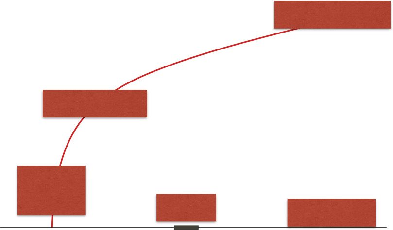
012107-7SCALLIET, BERTHIER, AND ZAMPONI PHYSICAL REVIEW E 99, 012107 (2019)
100 100
Unstable (a) (b)
10−1
10−1 Simple Glass
g2
−2
10
T
T
g1
10−2 Marginal
Glass 10−3
10−3 10−4
-1 0 1 2 3 -1 0 ηJ 1 2 3
ηJ η η
100 100
(c) (d)
10−1 g4
10−1
g3
10−2
T
T
10−2
10−3
10−3 10−4
-1 0 1 2 3 4 -1 ηJ 0 1 2 3 4
ηJ η η
FIG. 5. Mean-field state-following phase diagrams for four different starting harmonic glasses (a) g1 , (b) g2 , (c) g3 , and (d) g4 , whose
location in the equilibrium phase diagram is shown Fig. 1. The region of stability of the simple glass phase is delimited by the spinodal (dashed
gray line) and Gardner transition line (solid blue line). Above the spinodal, the glass melts into the liquid. Below the Gardner transition line,
the glass is marginally stable (shaded blue region). The jamming transition of the glasses takes place at T = 0 and ηJ indicated by an arrow.
range of state points. Finally, all these glasses also become limit of the WCA model, where only the repulsive part of the
marginal when compressed to large packing fractions far Lennard-Jones interaction is physically relevant. We follow
above jamming. the strategy and representation adopted in Sec. IV B for the
The phase diagrams found in Fig. 5 suggest the existence harmonic spheres.
of two types of behaviors. Some glasses undergo a Gardner The thermodynamic state of IPL glasses only depends on
transition as they are cooled, while some glasses do not. This the combination = ϕ̂/T 1/4 . The complete phase diagram
distinction depends both on the initial temperature Tg of the for the IPL model can therefore be completely understood
glass and on its initial density ϕ̂g . To distinguish between these
two types of glasses, we define a line TX (ϕ̂g ) which delimits
in the (Tg , ϕ̂g ) phase diagram. Our results for TX are reported
in Fig. 6. Glasses prepared in the shaded part of this phase
diagram, like g2 and g3 , undergo a Gardner transition to a
marginally stable phase upon cooling at constant density. The
other glasses, like g1 and g4 , do not and remain stable glasses
down to T = 0. The corresponding phase diagram presented
in Fig. 6 is rather complex, exhibiting nonmonotonic reentrant
lines TX . The mean-field phase diagram of soft repulsive
spheres is therefore not a trivial extension of the one of hard
spheres. Figure 6 shows that a Gardner phase is relevant for
hard-sphere glasses, for soft particles prepared not too far
from either the dynamical transition Td and the temperature
TJ , which suggests two distinct possible physical origins for
the Gardner phase.
FIG. 6. Equilibrium mean-field phase diagram of harmonic
D. Dense liquid regime
spheres, as in Fig. 2. We add the transition lines TX (thin lines)
We now focus on the dense liquid regime modeled by which delimit the glasses that become unstable upon cooling (shaded
the IPL potential. This also corresponds to the high-density region), such as g2 and g3 , or not, as for g1 and g4 .
012107-8MARGINALLY STABLE PHASES IN MEAN-FIELD … PHYSICAL REVIEW E 99, 012107 (2019)
In this dense liquid regime, glasses prepared at Tg < 0.567
Td remain stable down to their ground state at T = 0, as reported
1 before [40]. The most stable glass for which we report the
Gardner transition line in Fig. 7 is Tg = 0.6. Below this
value, glasses remain stable in the entire phase diagram and
never undergo a transition to a marginally stable phase, even
T
at arbitrarily high compressions. This is consistent with the
0.5 high-density high-temperature limit found in the harmonic
phase diagram Fig. 6, where only glasses prepared in the
vicinity of the dynamical transition become marginally stable
upon cooling (shaded region). However, harmonic spheres
0 are qualitatively distinct from both the WCA model and
-1 -0.5 0 0.5 1 1.5 2 IPL potential regarding compression of very stable glasses:
η Whereas harmonic spheres always reach marginal states upon
compression at constant temperature, very stable WCA and
FIG. 7. Dense liquid regime analyzed using the IPL potential. IPL glasses do not. Note also that for harmonic spheres, the
Glasses prepared at ϕ̂g = 4.304 (Td = 1) for various Tg = 0.9, 0.8,
Gardner and spinodal lines meet at high density, so the glass
0.7, and 0.6 are followed in the (T , η) plane. For each glass, we
always melts upon high enough compression, which is not the
represent the state-following Gardner transition line TG (η) (solid
case of the WCA and IPL models.
lines) and the spinodal (dashed lines). All lines obey T ∼ e4η . The
marginal phase shifts to high density and lower temperatures as Tg
decreases, and disappears altogether for Tg < 0.567.
V. DISCUSSION AND PERSPECTIVES
In this work we have obtained the complete mean-field
phase diagrams of several glass-forming models. In particular,
by fixing, for instance, the packing fraction and changing the we provided detailed information regarding the location of the
temperature of the glass. For convenience, we choose ϕ̂g = marginally stable glass phases for a variety of pair interac-
4.304, for which the dynamical transition takes place at Td = tions and physical conditions, extensively exploring physical
1. We consider glasses with different stabilities, prepared at regimes relevant to granular materials, foams, emulsions, hard
Tg < Td . Despite the one-dimensional nature of the phase and soft colloids, and molecular glasses. We find that all
diagram, we show results for IPL glasses using the same types of glasses may become marginally stable upon cooling
representation as for harmonic spheres, using both T and η, or compression, but the extent of marginal phases strongly
to allow for a more direct comparison of the two types of depends on the preparation protocol and the chosen model. We
models. By definition, all lines in this diagram exactly obey find that increasing the glass stability systematically reduces
the relation T ∝ e4η . the extent of marginality. For well-annealed glasses, we find
†
We find that glasses prepared at Tg < Tg 0.92 transform that marginality emerges in two distinct regions, either around
into a marginally stable glass when cooled. Instead, glasses the jamming transition or at high compression. Our results
†
prepared in the range Tg < Tg < Td first transform into a suggest that marginal phases should be easily observable for
1RSB glass. As for harmonic spheres, the slope (λ) ˙ is colloidal and non-Brownian particles near jamming or for
† †
negative for Tg < Tg , diverges upon approaching Tg from poorly annealed glasses.
below, and is formally positive above it. The Gardner tran- Our study unifies previous results on marginal stability
sition lines for glasses prepared at Tg = 0.9, 0.8, 0.7, and in mean-field models [25,26,39,40]. Already in mean-field
0.6 are presented in Fig. 7. They have the form TG (η) = theory, marginal stability emerges under distinct physical
TG (η = 0)e4η , where TG (η = 0) is the Gardner transition conditions in different microscopic models. This provides
temperature obtained for a simple cooling of the glass. The a way to reconcile apparently contradictory numerical and
breaking point λ at the Gardner transition is equal to λ = experimental studies aimed at detecting Gardner phases in
0.407, 0.283, 0.168, and 0.042 for Tg = 0.9, 0.8, 0.7, and finite-dimensional glasses, where its existence is still debated
0.6, respectively. As for harmonic spheres, λ → 0 when TG [70,71]. In particular, the evidence for marginally stable
vanishes. The marginally stable phase is pushed to higher phases reported for two- and three-dimensional hard-sphere
densities and lower temperatures (in fact, to larger ) as the glasses under compression contrasts with its absence in two-
glass stability increases. In this model, however, particles do and three-dimensional numerical models of dense liquids
not possess a physical size (the potential has no cutoff at a upon cooling. Our analysis shows that already at the mean-
finite distance) and hence the jamming transition cannot be field level these two types of systems behave differently. In
observed. As a consequence, the domes of marginal stability addition, while the critical properties around the jamming
found around the jamming transition in Figs. 4 and 5 for transition remain unchanged from d = ∞ down to d = 2
harmonic spheres are absent for the IPL model. The behavior [72,73], the nature of the mean-field dynamical transition
of the Gardner transition lines at high η with decreasing Tg is highly altered by finite-dimensional fluctuations [74]. For
is similar in the IPL and WCA models. The WCA potential instance, our results predict that highly compressed dense
instead behaves as harmonic spheres near jamming and is thus liquids should be marginally stable (see also [41]), a protocol
characterized by domes around jamming. that was never tested in finite-dimensional studies.
012107-9SCALLIET, BERTHIER, AND ZAMPONI PHYSICAL REVIEW E 99, 012107 (2019)
Our results will be useful to guide future numerical simu- length would also develop in the contact network [75]. The
lations and experiments aimed at detecting marginally stable absence of thermal fluctuations should make the study of this
phases in finite-dimensional glasses. We find that mean-field transition much easier than in the thermal case.
Gardner phases are not restricted to exist in the immediate While the nature of the mean-field Gardner transition is
vicinity of jamming and could be more broadly relevant to a certainly affected in finite dimensions [70], the existence
wide class of materials. We are currently numerically investi- of extended marginally stable phases should give rise to
gating, along the lines of this theoretical work, the evolution interesting new physics in structural glasses. As happens in
of the Gardner transition while continuously interpolating spin glasses, even if the Gardner phase transition is avoided
between regimes relevant to dense hard-sphere glasses and in physical dimensions [48], it may still be the case that
dense liquids, using a WCA potential [49]. interesting physical phenomena, such as aging and nonlinear
Our results open a number of additional perspectives for fu- dynamics, remain relevant to describe the behavior of struc-
ture work. One finding is that soft-sphere glasses can undergo tural glasses.
a zero-temperature Gardner transition, as reported in Fig. 5. A
convenient protocol to observe this transition is suggested in
ACKNOWLEDGMENTS
Fig. 5(d) for the glass g4 . It can be quenched at T = 0, where it
is jammed and in the simple glass phase. It is therefore a stable We thank G. Biroli and P. Urbani for useful exchanges.
harmonic energy minimum. Under decompression at T = 0, F.Z. and L.B. thank the ICTS, Bangalore for kind hospital-
this state undergoes a Gardner transition before unjamming. ity during the last stages of writing the paper. This work
The signature of this zero-temperature Gardner transition, if was supported by the Simons Foundation through Grants
it exists in two or three dimensions, would be particularly No. 454933 (L.B.) and No. 454955 (F.Z.). This project has
dramatic: The Hessian would develop delocalized soft modes received funding from the European Research Council under
[32] and the system would start responding by intermittent the European Union’s Horizon 2020 research and innovation
avalanches [35] to an applied strain. A divergent correlation program (Grant Agreement No. 723955, GlassUniversality).
[1] A. J. Liu and S. R. Nagel, Nature (London) 396, 21 (1998). [19] M. Wyart, L. E. Silbert, S. R. Nagel, and T. A. Witten,
[2] A. J. Liu and S. R. Nagel, Jamming and Rheology: Constrained Phys. Rev. E 72, 051306 (2005).
Dynamics on Microscopic and Macroscopic Scales (Taylor & [20] M. Müller and M. Wyart, Annu. Rev. Condens. Matter Phys. 6,
Francis, London, 2001). 177 (2015).
[3] A. Cavagna, Phys. Rep. 476, 51 (2009). [21] T. R. Kirkpatrick and P. G. Wolynes, Phys. Rev. A 35, 3072
[4] L. Berthier and G. Biroli, Rev. Mod. Phys. 83, 587 (2011). (1987).
[5] A. J. Liu and S. R. Nagel, Annu. Rev. Condens. Matter Phys. 1, [22] T. R. Kirkpatrick and D. Thirumalai, Phys. Rev. Lett. 58, 2091
347 (2010). (1987).
[6] A. J. Liu, S. R. Nagel, W. Van Saarloos, and M. Wyart, in [23] M. Mezard and G. Parisi, in Structural Glasses and Supercooled
Dynamical Heterogeneities and Glasses, edited by L. Berthier, Liquids: Theory, Experiment and Applications, edited by P. G.
G. Biroli, J.-P. Bouchaud, L. Cipelletti, and W. van Saarloos Wolynes and V. Lubchenko (Wiley, New York, 2012).
(Oxford University Press, Oxford, 2011). [24] Structural Glasses and Supercooled Liquids: Theory, Exper-
[7] L. Berthier and T. A. Witten, Phys. Rev. E 80, 021502 (2009). iment, and Applications, edited by V. Lubchenko and P. G.
[8] A. Ikeda, L. Berthier, and P. Sollich, Phys. Rev. Lett. 109, Wolynes (Wiley, New York, 2012).
018301 (2012). [25] J. Kurchan, G. Parisi, P. Urbani, and F. Zamponi, J. Phys. Chem.
[9] R. Mari, F. Krzakala, and J. Kurchan, Phys. Rev. Lett. 103, B 117, 12979 (2013).
025701 (2009). [26] P. Charbonneau, J. Kurchan, G. Parisi, P. Urbani, and F.
[10] P. Chaudhuri, L. Berthier, and S. Sastry, Phys. Rev. Lett. 104, Zamponi, Annu. Rev. Condens. Matter Phys. 8, 265 (2017).
165701 (2010). [27] D. J. Gross, I. Kanter, and H. Sompolinsky, Phys. Rev. Lett. 55,
[11] G. Parisi and F. Zamponi, Rev. Mod. Phys. 82, 789 (2010). 304 (1985).
[12] M. Ozawa, T. Kuroiwa, A. Ikeda, and K. Miyazaki, Phys. Rev. [28] E. Gardner, Nucl. Phys. B 257, 747 (1985).
Lett. 109, 205701 (2012). [29] M. Mézard, G. Parisi, and M. A. Virasoro, Spin Glass Theory
[13] R. C. Zeller and R. O. Pohl, Phys. Rev. B 4, 2029 (1971). and Beyond (World Scientific, Singapore, 1987).
[14] D. G. Cahill and R. O. Pohl, Annu. Rev. Phys. Chem. 39, 93 [30] L. Berthier, P. Charbonneau, Y. Jin, G. Parisi, B. Seoane, and
(1988). F. Zamponi, Proc. Natl. Acad. Sci. USA 113, 8397 (2016).
[15] L. E. Silbert, A. J. Liu, and S. R. Nagel, Phys. Rev. Lett. 95, [31] A. Ikeda, L. Berthier, and G. Biroli, J. Chem. Phys. 138,
098301 (2005). 12A507 (2013).
[16] E. Lerner, E. DeGiuli, G. Düring, and M. Wyart, Soft Matter [32] S. Franz, G. Parisi, P. Urbani, and F. Zamponi, Proc. Natl. Acad.
10, 5085 (2014). Sci. USA 112, 14539 (2015).
[17] P. Charbonneau, E. I. Corwin, G. Parisi, A. Poncet, and F. [33] S. Franz, T. Maimbourg, G. Parisi, and A. Scardicchio,
Zamponi, Phys. Rev. Lett. 117, 045503 (2016). arXiv:1811.11719.
[18] M. Wyart, S. R. Nagel, and T. A. Witten, Europhys. Lett. 72, [34] G. Biroli and P. Urbani, Nat. Phys. 12, 1130 (2016).
486 (2005). [35] S. Franz and S. Spigler, Phys. Rev. E 95, 022139 (2017).
012107-10MARGINALLY STABLE PHASES IN MEAN-FIELD … PHYSICAL REVIEW E 99, 012107 (2019)
[36] Y. Jin and H. Yoshino, Nat. Commun. 8, 14935 (2017). [57] C. Rainone, P. Urbani, H. Yoshino, and F. Zamponi, Phys. Rev.
[37] H. G. E. Hentschel, S. Karmakar, E. Lerner, and I. Procaccia, Lett. 114, 015701 (2015).
Phys. Rev. E 83, 061101 (2011). [58] W. Götze, Complex Dynamics of Glass-Forming Liquids: A
[38] I. Procaccia, C. Rainone, C. A. B. Z. Shor, and M. Singh, Mode-Coupling Theory (Oxford University Press, New York,
Phys. Rev. E 93, 063003 (2016). 2009), Vol. 143.
[39] G. Biroli and P. Urbani, SciPost Phys. 4, 20 (2018). [59] T. Maimbourg, J. Kurchan, and F. Zamponi, Phys. Rev. Lett.
[40] C. Scalliet, L. Berthier, and F. Zamponi, Phys. Rev. Lett. 119, 116, 015902 (2016).
205501 (2017). [60] C. Rainone and P. Urbani, J. Stat. Mech. (2016) 053302.
[41] V. Lubchenko and P. G. Wolynes, J. Phys. Chem. B 122, 3280 [61] H.-J. Sommers, J. Phys. Lett. 46, 779 (1985).
(2017). [62] S. Franz, G. Parisi, M. Sevelev, P. Urbani, F. Zamponi, and
[42] P. Charbonneau, E. I. Corwin, L. Fu, G. Tsekenis, and M. van M. Sevelev, SciPost Phys. 2, 019 (2017).
der Naald, arXiv:1802.07391. [63] F. Caltagirone, U. Ferrari, L. Leuzzi, G. Parisi, F. Ricci-
[43] B. Seoane and F. Zamponi, Soft Matter 14, 5222 (2018). Tersenghi, and T. Rizzo, Phys. Rev. Lett. 108, 085702 (2012).
[44] A. Seguin and O. Dauchot, Phys. Rev. Lett. 117, 228001 [64] S. Franz, H. Jacquin, G. Parisi, P. Urbani, and F. Zamponi, Proc.
(2016). Natl. Acad. Sci. USA 109, 18725 (2012).
[45] Q. Liao and L. Berthier, arXiv:1810.10256. [65] G. Parisi and T. Rizzo, Phys. Rev. E 87, 012101 (2013).
[46] B. Seoane, D. R. Reid, J. J. de Pablo, and F. Zamponi, [66] G. Parisi, F. Ricci-Tersenghi, and T. Rizzo, J. Stat. Mech. (2014)
Phys. Rev. Mater. 2, 015602 (2018). P04013.
[47] K. Geirhos, P. Lunkenheimer, and A. Loidl, Phys. Rev. Lett. [67] S. S. Dalal and M. D. Ediger, J. Phys. Chem. Lett. 3, 1229
120, 085705 (2018). (2012).
[48] C. L. Hicks, M. J. Wheatley, M. J. Godfrey, and M. A. Moore, [68] M. D. Ediger, J. Chem. Phys. 147, 210901 (2017).
Phys. Rev. Lett. 120, 225501 (2018). [69] C. J. Fullerton and L. Berthier, Europhys. Lett. 119, 36003
[49] C. Scalliet, L. Berthier, and F. Zamponi (unpublished). (2017).
[50] D. J. Durian, Phys. Rev. Lett. 75, 4780 (1995). [70] P. Urbani and G. Biroli, Phys. Rev. B 91, 100202 (2015).
[51] D. Ruelle, Statistical Mechanics: Rigorous Results (World [71] P. Charbonneau and S. Yaida, Phys. Rev. Lett. 118, 215701
Scientific, Singapore, 1999). (2017).
[52] M. Skoge, A. Donev, F. H. Stillinger, and S. Torquato, [72] C. P. Goodrich, A. J. Liu, and S. R. Nagel, Phys. Rev. Lett. 109,
Phys. Rev. E 74, 041127 (2006). 095704 (2012).
[53] J. A. van Meel, B. Charbonneau, A. Fortini, and P. [73] P. Charbonneau, E. I. Corwin, G. Parisi, and F. Zamponi,
Charbonneau, Phys. Rev. E 80, 061110 (2009). Phys. Rev. Lett. 114, 125504 (2015).
[54] S. Franz and G. Parisi, J. Phys. (France) I 5, 1401 (1995). [74] T. R. Kirkpatrick, D. Thirumalai, and P. G. Wolynes, Phys. Rev.
[55] L. Zdeborová and F. Krzakala, Phys. Rev. B 81, 224205 (2010). A 40, 1045 (1989).
[56] F. Krzakala and L. Zdeborová, Europhys. Lett. 90, 66002 [75] D. Hexner, A. J. Liu, and S. R. Nagel, Phys. Rev. Lett. 121,
(2010). 115501 (2018).
012107-11You can also read