A Landau-de Gennes theory for twist-bend and splay-bend nematic phases of colloidal suspensions of bent rods
←
→
Page content transcription
If your browser does not render page correctly, please read the page content below
A Landau–de Gennes theory for twist-bend
and splay-bend nematic phases of colloidal
suspensions of bent rods
Cite as: J. Chem. Phys. 152, 224502 (2020); https://doi.org/10.1063/5.0008936
Submitted: 26 March 2020 . Accepted: 17 May 2020 . Published Online: 08 June 2020

Carmine Anzivino      , René van Roij     , and Marjolein Dijkstra

ARTICLES YOU MAY BE INTERESTED IN

Inverse methods for design of soft materials
The Journal of Chemical Physics 152, 140902 (2020); https://doi.org/10.1063/1.5145177

Dynamics of poly[n]catenane melts
The Journal of Chemical Physics 152, 214901 (2020); https://doi.org/10.1063/5.0007573

Surveying the free energy landscape of clusters of attractive colloidal spheres
The Journal of Chemical Physics 152, 134901 (2020); https://doi.org/10.1063/1.5144984

J. Chem. Phys. 152, 224502 (2020); https://doi.org/10.1063/5.0008936                152, 224502

© 2020 Author(s).

The Journal
                                                                                                  ARTICLE            scitation.org/journal/jcp
 of Chemical Physics

    A Landau–de Gennes theory for twist-bend
    and splay-bend nematic phases of colloidal
    suspensions of bent rods
    Cite as: J. Chem. Phys. 152, 224502 (2020); doi: 10.1063/5.0008936
    Submitted: 26 March 2020 • Accepted: 17 May 2020 •
    Published Online: 8 June 2020

    Carmine Anzivino,1,a)                   René van Roij,2   and Marjolein Dijkstra1,b)

    AFFILIATIONS
    1
      Soft Condensed Matter, Debye Institute for Nanomaterial Science, Utrecht University, Princetonplein 1, Utrecht 3584 CC, The
      Netherlands
    2
      Institute for Theoretical Physics, Center for Extreme Matter and Emergent Phenomena, Utrecht University, Princetonplein 5,
      Utrecht 3584 CC, The Netherlands

    a)
         Author to whom correspondence should be addressed: c.anzivino@uu.nl
    b)
         Electronic mail: m.dijkstra@uu.nl

    ABSTRACT
    We develop a phenomenological Landau–de Gennes (LdG) theory for lyotropic colloidal suspensions of bent rods using a Q-tensor expansion
    of the chemical-potential dependent grand potential. In addition, we introduce a bend flexoelectric term, coupling the polarization and the
    divergence of the Q-tensor, to study the stability of uniaxial (N), twist-bend (N TB ), and splay-bend (N SB ) nematic phases of colloidal bent
    rods. We first show that a mapping can be found between the LdG theory and the Oseen–Frank theory. By breaking the degeneracy between
    the splay and bend elastic constants, we find that the LdG theory predicts either an N–N TB –N SB or an N–N SB –N TB phase sequence upon
    increasing the particle concentration. Finally, we employ our theory to study the first-order N–N TB phase transition, for which we find that
                                              eff                                             eff
    K 33 as well as its renormalized version K33  remain positive at the transition, whereas K33  vanishes at the nematic spinodal. We connect these
    findings to recent simulation results.
    Published under license by AIP Publishing. https://doi.org/10.1063/5.0008936., s

    I. INTRODUCTION                                                           bent-core molecules in the absence of electric fields. As a result, it is
                                                                              particularly easy to induce bend deformations in the nematic direc-
           Bent-core liquid crystals are mesophases formed by molecules       tor field of bent-core liquid crystals. Many years later, Dozov3 noted
    with a “banana-like” shape.1 In the simplest liquid-crystal phase,        that the bend elastic constant K 33 can be very small for bent-core
    i.e., the uniaxial nematic (N) phase, the long axes of the bent-core      liquid crystals, yielding a low energy cost for bend deformations. In
    molecules are preferentially aligned along a common direction, the        addition, Dozov speculated that K 33 could also become negative in
    so-called nematic director n̂, and the transverse orientations of the     certain bent-core liquid crystals. In this case, higher-order terms in
    molecules are randomly oriented in the plane perpendicular to n̂.         the derivatives of the nematic director field (beyond linear elastic-
    In addition to the N phase with an orientational order of the main        ity) should be included in the free energy in order to stabilize the
    molecular axis, the molecular shape can stabilize a nematic phase         system. The competition between the putative negative K 33 term
    with polar order, in which the transverse orientations exhibit a net      and the positive higher-order terms would favor spontaneous bend
    alignment in a direction perpendicular to n̂. In 1969, Meyer2 argued      deformations. Interestingly, however, the theoretical work of Dozov
    that the polar order of the transverse directions couples to the bend     did not consider any polar order. Since it is impossible to extend a
    deformations of the nematic director n̂ through a mechanism called        pure bend deformation in three-dimensional space, Meyer as well
    the bend flexoelectric effect. The polar order and the bend flexoelec-    as Dozov predicted that the uniaxial N phase can become unsta-
    tric effect may occur in liquid crystals due to electrostatic polariza-   ble with respect to either a spatially modulated twist-bend nematic
    tion and may also arise due to the molecular shape in systems of          (N TB ) phase, characterized by a heliconical variation with bend and

J. Chem. Phys. 152, 224502 (2020); doi: 10.1063/5.0008936                                                                                  152, 224502-1
Published under license by AIP Publishing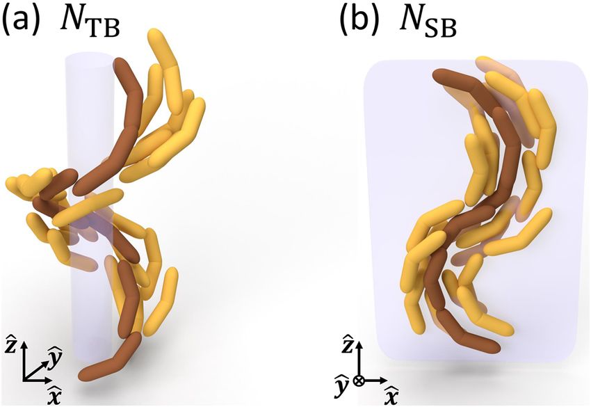
The Journal
                                                                                                                  ARTICLE              scitation.org/journal/jcp
 of Chemical Physics

    twist deformations in the molecular orientation [see Fig. 1(a)], or a                    bend elastic constant before the onset of the polar order in bent-core
    modulated splay-bend nematic (N SB ) phase, characterized by alter-                      liquid crystals, in agreement with Selinger et al.5–7
    nating domains of splay and bend3,4 [see Fig. 1(b)]. Quantitatively,                           Much research in recent years has been focused on ther-
    Dozov’s theory, based on the Oseen–Frank elastic theory, predicts                        motropic bent-core mesogens that become liquid crystalline upon
    that the uniaxial N phase becomes unstable to the formation of N TB                      lowering the temperature. Very recently, various routes have been
    or N SB phases at a critical point corresponding to K 33 = 0, where                      developed to synthesize lyotropic colloidal model systems of bent-
    the system either stabilizes an N TB phase if K 11 > 2K 22 or an N SB                    core molecules, e.g., silica rods with a sharp kink31–33 or smoothly
    phase if K 11 < 2K 22 , with K 11 and K 22 being the splay and twist elastic             curved SU-8 rods.34 The liquid crystalline behavior of these colloidal
    constants, respectively.3                                                                systems is driven by concentration and has been studied by simula-
          Recently, Selinger and collaborators5–7 suggested that the pres-                   tions and microscopic theories. Using Onsager theory,35 a first-order
    ence of polar order could provide the simplest explanation not only                      uniaxial N to N TB phase transition has been predicted recently in a
    for the formation of spatially modulated phases, in agreement with                       system of hard curved particles at sufficiently high particle concen-
    Meyer, but also for the negative bend elastic constant K 33 proposed                     trations,19 which has been confirmed in computer simulations19,36
    by Dozov. These authors introduced a Landau theory that com-                             on systems of hard bent spherocylinders. In addition, this simu-
    bines the Oseen–Frank free energy for the nematic director n̂, the                       lation study showed that the N–N TB phase transition is followed
    polar order P perpendicular to n̂, and the coupling between the                          by a second-order N TB –N SB phase transition in a polydisperse sys-
    polar order and bend deformations. By minimizing the free energy                         tem of hard bent spherocylinders and in a system of hard curved
    with respect to the polar order, they obtained Dozov’s effective free                    particles.
    energy in terms of only the nematic director field n̂ with renormal-                           In this paper, we extend the existing LdG theories of ther-
    ized elastic constants. In this picture, K 33 remains always positive,                   motropic bent-core liquid crystals to lyotropic liquid crystals in
                                         eff                                                 order to develop a framework to describe the recent findings of Refs.
    while its renormalized version K33       decreases in magnitude and van-
    ishes at a critical point where the uniaxial N phase becomes unstable                    19 and 36. To this end, we introduce a chemical-potential dependent
    with respect to the N TB or N SB phase. Interestingly, they also found                   grand potential based on a Q-tensor expansion and a bend flexo-
    the same criterion for the relative stability of the spatially modu-                     electric term coupling the polarization and the divergence of the
    lated phases calculated by Dozov,6 i.e., K 11 < 2K 22 for an N SB phase                  Q-tensor.8–12 We first show that a mapping can be found between
    and K 11 > 2K 22 for an N TB phase. Finally, Selinger’s theory has                       the LdG theory and the Oseen–Frank theory of Selinger and co-
    been extended8–12 to a mesoscopic Landau–de Gennes (LdG) the-                            workers.6,7 We then show, by breaking the degeneracy between the
    ory where the director n̂ is replaced by a second rank, symmetric,                       splay and bend elastic constants, that the LdG theory predicts a series
    and traceless tensor Q(r) with components Qαβ (r), where α, β = 1, 2,                    of second-order phase transitions between periodically modulated
    3 represent the Cartesian coordinates.                                                   nematic phases, reproducing what was found in Ref. 36. Finally, we
          For completeness, we also mention that theories have been                          employ our theory to study the first-order N–N TB phase transition
    developed for bent-core liquid crystals that do not involve spon-                        observed in simulations. We find that while the LdG theory predicts
                                                                                                                  eff
    taneous polar order or a negative bend elastic constant.13–18 Addi-                      that K 33 > 0 and K33    = 0 at a second-order N–N TB phase transition,
    tionally, molecular field approaches19–30 for bent-core liquid crystals                  it also predicts that K 33 as well as K33eff
                                                                                                                                          remains positive at a first-order
    exist, of which several20,26,28–30 support the idea of softening of the                                                     eff
                                                                                             N–N TB transition, whereas K33 vanishes at the nematic spinodal.
                                                                                                   As a final introductory remark, it is worth mentioning that the
                                                                                             splay-bend nematic phase considered in this paper differs from the
                                                                                             so-called splay nematic (N S ) phase considered in Refs. 12, 37, and
                                                                                             38. This N S phase is characterized by a modulation perpendicular to
                                                                                             the average director, while the N SB phase is characterized by a spa-
                                                                                             tial modulation parallel to the global nematic director. Moreover,
                                                                                             the onset of the N S phase is driven by softening of the renormal-
                                                                                                                              eff
                                                                                             ized splay elastic constant K11      rather than of the renormalized bend
                                                                                                                 eff
                                                                                             elastic constant K33 .
                                                                                                   The outline of this paper is as follows: Sec. II describes our LdG
                                                                                             theory. In Sec. III, we briefly review the isotropic-nematic phase
                                                                                             transition of hard rods within this framework, which will be used
                                                                                             as a reference system throughout this paper. In Sec. IV, we investi-
                                                                                             gate possible phase sequences of the spatially modulated phases. The
                                                                                             first-order N–N TB transition is studied in Sec. V, and the renormal-
                                                                                             ized elastic constants are derived in Sec. VI. Finally, we present our
                                                                                             conclusions and a discussion in Sec. VII.

      FIG. 1. (a) Twist-bend nematic (NTB ) phase characterized by a heliconical variation   II. LANDAU–de GENNES THEORY
      of the particle orientation along the z-axis. (b) Splay-bend nematic (NSB ) phase            LdG theory is based on the hypothesis that equilibrium prop-
      characterized by alternating domains of splay and bend in the x-z plane.
                                                                                             erties of a thermodynamic system can be found from a variational

J. Chem. Phys. 152, 224502 (2020); doi: 10.1063/5.0008936                                                                                                      152, 224502-2
Published under license by AIP Publishing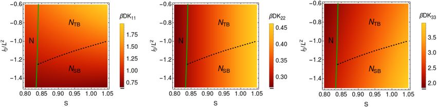
The Journal
                                                                                                  ARTICLE            scitation.org/journal/jcp
 of Chemical Physics

    Helmholtz (or Gibbs) free energy F, constructed as an expansion in        where Δωb ≡ Δωb (Q; μ) is the excess bulk grand potential density
    powers of a suitable order parameter. A restriction on the expan-         with respect to the I state, ωe ≡ ωe (Q, ∇Q) describes elastic defor-
    sion is that it must be stable against an unlimited growth of the         mations and surface tension effects, and ωP ≡ ωP (Q, P, ∇Q, ∇P)
    order parameter. It is well known39 that the orientational order          contains additionally lowest order couplings between Q and the
    of three-dimensional nematic liquid crystals can be described by a        polarization field P and its derivatives ∂ α Pβ .
    second-rank, symmetric, traceless tensor field, Q(r), with cartesian           We expand the bulk contribution in units of β−1 = kB T with kB
    components Qαβ (r) for α, β = 1, 2, 3, which vanishes in the isotropic    being the Boltzmann constant, until fourth order in Q, which gives
    (I) phase and thus serves as an order parameter for the N phase. The      us
    eigenvector of Q corresponding to the maximum modulus of a non-
    degenerate eigenvalue defines the nematic director n̂ of the system.                            2                     4
                                                                                    βB2 Δωb (Q; μ) = aβ(μ∗ − μ)Qαβ Qβα − b Qαβ Qβλ Qλα
    The variational LdG free energy F for ordinary, non-chiral nematics                             3                     3
    is constructed from frame-invariant contractions of Qαβ and spatial                               4
                                                                                                    + d Qαβ Qβα Qλρ Qρλ ,                          (2)
    derivatives ∂ λ Qαβ such as Qαβ Qβα , Qαβ Qβλ Qλα , with phenomeno-                               9
    logical coefficients that contain the dependence on the thermody-
    namic state (pressure and temperature). Usually for thermotropic          where we use Einstein’s summation convention for repeated indices
    liquid crystals, only the quadratic term of the Landau expansion          throughout this paper. The second virial coefficient in the isotropic
    changes sign as a function of temperature, which drives the phase         fluid phase is given by B2 = πL2 D/4 in the limit L ≫ D and is included
    transition.40–42                                                          in our definition to render the Landau coefficients a, b, and d con-
          In contrast to “ordinary” nematics, a proper characterization       veniently dimensionless. For simplicity, we assume them to be inde-
    of orientational order exhibited by bent-core liquid-crystal phases       pendent of μ. We also introduce μ∗ , the chemical potential at which
    requires additional order parameters. In the case of theories based       the quadratic term changes sign, i.e., it defines the spinodal of the
    on the flexoelectric effect, not only the tensor field Q(r) is required   I–N transition. A stable I phase at μ < μ∗ requires a > 0, the stability
    but also a vector field P(r) with cartesian components Pα (r) that        of expansion (2) with respect to an unlimited growth of Q requires
    describes the polar order in a direction perpendicular to n̂. In the      that d > 0, while b > 0 allows us to describe a first-order I–N transi-
    I phase, Q = 0 and P = 0; in the uniaxial N phase, Q ≠ 0 and P = 0;       tion to a state with Q≠0. Throughout, we will satisfy these stability
    and in the spatially modulated nematic phases, Q ≠ 0 and P ≠ 0.           criteria.
    General O(3)-symmetric extensions of the free energy F that con-                For the terms in gradients of Q, we only retain terms up to
    tain additionally lowest order couplings with P and its derivatives       the square gradients in Q, and we consider only one of the possi-
    ∂ α Pβ have been developed in Refs. 8–12. However, these expan-           ble invariants that involve the coupling between the order parameter
    sions are only suitable for thermotropic systems that become liquid       Q and quadratic gradient in Q to break the degeneracy between the
    crystalline as a function of temperature. In contrast, lyotropic sys-     splay and bend elastic constants K 11 and K 33 .46 We thus write
    tems become ordered as a function of density and are not conve-                              2                       2
    niently described by the Helmholtz free energy F. A naive remedy             βB2 ωe (Q, ∇Q) = l1 (∂α Qβλ )(∂α Qβλ ) + l2 (∂α Qαλ )(∂β Qβλ )
    for this problem would be to replace the temperature in F by the                             9                       9
                                                                                                    2
    density ρ, but this cannot capture the density jumps that are found                          − l3 Qαβ (∂γ Qαγ )(∂ξ Qβξ ),                   (3)
    at first-order transitions, which for the I–N phase transition can                              9
    be as large as 25%.43 The density discontinuity at the I–N transi-        where we omitted another second-order term in ∇Q, which scales
    tion is instead exhibited by microscopic theories, such as Onsager        with (∂ α Qβλ )(∂ λ Qβα ) because it can be written as a linear combina-
    theory.                                                                   tion of a surface term and the elastic terms already included in the
          Here, we follow Ref. 44 and set up a Landau expansion for           expansion (3). We express the expansion parameters l1 , l2 , and l3
    lyotropics for which we will use the grand potential Ω rather than        in units of L2 throughout this paper. We note again that we have
    the Helmholtz (or Gibbs) free energy F. By using Ω, the expansion         chosen only one of the possible couplings between Q and ∇Q to
    parameters will depend on the chemical potential μ, and the density       break the degeneracy between K 11 and K 33 .46 This choice is arbi-
    jumps will naturally be encoded through the relation ∂(Ω/V)/∂μ|V ,T       trary; in addition, other terms could have been considered or even
    = −ρ, with V being the volume of the system and ρ being the average       more terms could have been included. Since all couplings add a con-
    density. Only the quadratic term Qαβ Qβα has a μ-dependent prefac-        tribution proportional to S3 to the elastic constants, the predictions
    tor that changes sign to drive the phase transition. This procedure       of the theory are not affected by this choice.
    is easier to use than, for example, the phase-field-crystal method of          Expressing Q(r) in terms of a scalar order parameter S(r) and a
    Ref. 45, which produces terms that also explicitly depend on density,     nematic director field n(r),
    for which also an Euler–Lagrange equation for ρ needs to be solved,
    in addition to the one for Q.                                                                     3                   1
          We consider a system of hard bent rods modeled as curved or                        Qαβ (r) = S(r)(nα (r)nβ (r) − δαβ ),                  (4)
                                                                                                      2                   3
    kinked rods of contour length L and diameter D, at chemical poten-
    tial μ in a macroscopic volume V at fixed temperature T. We write         we can relate the parameters l1 , l2 , and l3 to the Oseen–Frank elas-
    the LdG grand potential as                                                tic constants through βDK11 = 4S2 (2l1 + l2 − Sl3 )/(πL2 ), βDK22
                                                                              = 8S2 l1 /(πL2 ), and βDK33 = 4S2 (2l1 + l2 + (S/2)l3 )/(πL2 ), respec-
                        ΔΩ(Q, P) = ∫ dr[Δωb + ωe + ωP ],               (1)    tively. These relations can be found by comparing the elastic
                                            V                                 expansion (3) using expression (4) with the Oseen–Frank elastic

J. Chem. Phys. 152, 224502 (2020); doi: 10.1063/5.0008936                                                                                  152, 224502-3
Published under license by AIP Publishing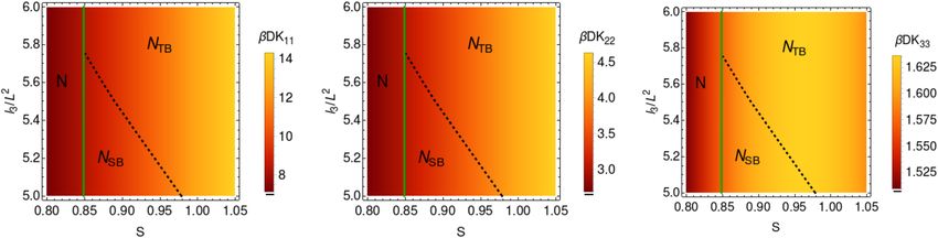
The Journal
                                                                                                            ARTICLE               scitation.org/journal/jcp
 of Chemical Physics

    energy,47,48                                                                       and unstable phases. We find the solutions
                         1                                                                           SI (μ) = 0;
                    F=          dr[K11 (∇ ⋅ n̂)2 + K22 (n̂ ⋅ ∇ × n̂)2
                         2∫                                                     (5)                                       √
                                                                                                                 3b ⎛             32adβ(μ∗ − μ) ⎞               (7)
                         + K33 ∣n̂ × (∇ × n̂)∣2 ],                                                   S±N (μ)   =     1±      1−                   ,
                                                                                                                 8d ⎝                  9b2      ⎠
    where K 11 , K 22 , and K 33 are the splay, twist, and bend elastic con-
    stants, respectively. We assume l1 , l2 , and l3 to be independent of              whose stability can be investigated by analyzing the sign of
    μ.                                                                                 ∂ 2 Δωb /∂S2 . We first note that from the conditions ∂ 2 Δωb /∂S2 ∣S=SI
         Finally, we expand ωP up to sixth order in P and write                        = 0, ∂ 2 Δωb /∂S2 ∣S=S+N = 0 and Δωb (SI ) = Δωb (S+N ), we can find
                                                                                       the chemical potential μ∗ corresponding to the spinodal of the I
                                                  2                                    phase with respect to the N phase, the chemical potential βμ+ = βμ∗
      βB2 ωP (Q, P, ∇Q, ∇P) = e2 Pα (δαβ +          Qαβ )Pβ
                                                 S0                                    − 9b/(32ad) corresponding to the spinodal of the N phase with
                                    + e4 Pα Pα Pβ Pβ − λPα (∂β Qαβ )                   respect to the I phase, and the chemical potential βμIN = βμ∗
                                    + κ(∂α Pβ )(∂α Pβ ) + e6 Pα Pα Pβ Pβ Pγ Pγ , (6)   − b2 /(4ad) corresponding to the I–N transition, respectively. We
                                                                                       then find that (i) for μ < μ+ , the I phase (SI ) is the stable configu-
    with coefficients e2 , e4 , e6 , κ, λ, and S0 . Throughout this paper, we          ration; (ii) for μ+ < μ < μIN , the I phase is stable, S−N is unstable, and
    will express λ and κ in terms of L and L2 , respectively. Stability in             S+N is metastable; (iii) for μIN < μ < μ∗ , the S+N solution is stable, the
    the dilute limit requires e2 > 0, while stability with respect to an               I phase is metastable, and S−N is unstable; and (iv) for μ > μ∗ , the S+N
    unlimited growth of P requires e6 > 0. The coefficients 2/S0 , λ, and              solution is stable, S−N is metastable, and the I phase is unstable. The
    κ represent the strength of the coupling between Q and P fields, the               solution S+N represents the N phase, and for the sake of simplicity, we
    flexoelectric coupling between P and gradients in Q, and a polar elas-             will use SN (μ) ≡ S+N (μ) throughout this paper.
    tic constant, respectively. In order to describe a favored polarization                  In order to describe the I–N transition of hard rods, we first
    perpendicular to the nematic director, leading to bend flexoelec-                  convert the chemical potential μ to the particle concentration c = B2 ρ
    tricity, we set S0 > 0.8 Finally, we allow e4 to be positive as well as            and then fit the phenomenological coefficients a, b, and d to results
    negative.                                                                          from Onsager theory.44 Concerning the first, we introduce the grand
          Our LdG expansion is very similar to those of Refs. 8 and 11.                potential density of the I state ωI and define ω ≡ ωI + Δωb . From the
    Nevertheless, in contrast to their work, and following the suggestion              condition ∂(B2 ω)/∂μ = −c, we then find
    of Ref. 7, we consider terms up to sixth order in P and simultane-
    ously allow the coefficient e4 of the fourth-order term in P to be                                           c(μ) = cI (μ) + aS2 (μ),                       (8)
    either positive or negative. This choice allows us to describe first-
                                                                                       where the particle concentration of the I phase cI (μ) = −∂(B2 ωI )/∂μ
    order as well as second-order transitions to the spatially modulated
                                                                                       can be calculated within Onsager theory, by using an isotropic dis-
    phases.49 In particular, if e4 < 0, we expect first-order phase transi-
                                                                                       tribution function, such that βμ(cI ) = log(cI /4π) + 2cI .50 By inverting
    tions, while if e4 ≥ 0, we expect second-order phase transitions. Our
                                                                                       this relation, we obtain cI (μ). For the fit of the phenomenological
    expansion includes the additional elastic term Qαβ (∂ γ Qαγ )(∂ ξ Qβξ ) to
                                                                                       coefficients a, b, and d, we exploit the thermodynamic quantities
    break the degeneracy between the splay and bend elastic constants
                                                                                       of the system at the I–N phase coexistence. Using Onsager theory
    K 11 and K 33 in agreement with Ref. 37. However, we note that Ref.
                                                                                       for a system of hard rods in the limit L/D → ∞,50,51 we find cI (μIN )
    37 lacks the term (∂ α Qαλ )(∂ β Qβλ ) and only considers terms up to
                                                                                       = 3.290, c(μIN ) = 4.191, βμ∗ = 6.855, βμIN = 5.241, and SIN = 0.7992.
    second-order in P. We also remark that our additional elastic term
                                                                                       Inserting these values into the following expressions:
    not only allows us to break the degeneracy between the splay and
    bend elastic constants but also enables us to change the ratio between                                      c(μIN ) = cI (μIN ) + aS2IN ,
    the splay and twist elastic constants K 11 /K 22 by varying the particle
    concentration. As will become clear in Sec. IV, this latter condition                                       βμIN = βμ∗ − b2 /(4ad),                         (9)
    is important for investigating the possibility of concentration-driven                                      SIN = b/(2d),
    phase transitions between the periodically modulated phases, as was
    recently found in simulations of hard particles.36                                 we obtain a = 1.436, b = 5.851, and d = 3.693. With this set of coef-
                                                                                       ficients, a plot of SI and SN as a function of the concentration c as
                                                                                       defined by Eq. (8) allows one to observe that the concentration jump
    III. I –N TRANSITION
                                                                                       associated with the I–N transition is correctly captured, as shown
          Here, we briefly review the LdG theory to describe the I–N tran-             in Ref. 44. Unless stated otherwise, we will use these values of a, b,
    sition of uniaxial hard rods as derived in Ref. 44. As stated in Sec. II,          d, and μ∗ in the following. We will also follow Ref. 44 in fitting the
    the uniaxial N phase is characterized by Q ≠ 0 and P = 0, and hence,               square-gradient coefficients l1 and l2 by using the surface tension of
    the ωP term in the grand potential (1) vanishes. We describe the bulk              a planar I–N interface of a system of hard rods with a parallel and
    uniaxial N phase by taking n̂ parallel to the z-axis. In this case, the            perpendicular anchoring, yielding l1 = 0.165L2 and l2 = 1.708L2 . We
    elastic expansion ωe = 0 and ΔΩ/V reduces to Δωb . Inserting the ten-              thus take a system of hard rods with L/D → ∞ as a reference sys-
    sor order parameter (4) with n̂ = (0, 0, 1) in (2), we obtain βB2 Δωb              tem for our study. Alternative reference systems are straightforward
    = aβ(μ∗ − μ)S2 − bS3 + dS4 . The Euler–Lagrange equation ∂Δωb /∂S                  to implement, provided that a sufficient number of quantities are
    = 0 can be solved analytically, in order to find the stable, metastable,           known at the bulk I–N transition.

J. Chem. Phys. 152, 224502 (2020); doi: 10.1063/5.0008936                                                                                               152, 224502-4
Published under license by AIP Publishing
The Journal
ARTICLE scitation.org/journal/jcp
of Chemical Physics
IV. SPATIALLY MODULATED PHASES Inserting Eqs. (12) and (13) back into Eq. (1) and approximating for
In this section, we study the phase behavior of lyotropic sus- small P, we find the grand potential density of the N TB phase,
pensions of bent rods by employing the LdG theory introduced in ΔΩTB ΔΩ ΔΩN
Sec. II with e6 = 0 and e4 > 0 in Eq. (6), i.e., using the formalism = −
V V V
for second-order phase transitions. We show that if l3 ≠ 0 in Eq. (3), e2 (S0 − S) 9λ2
the LdG theory predicts that an N–N TB –N SB and an N–N SB –N TB =[ − ]P2
S0 8(2l1 + l2 )
phase sequence can be stabilized in this system upon increasing the √
nematic order, in addition to the N–N TB and N–N SB transitions 9λ2 κS2 l1
+ 2 ∣P∣3 + e4 P4 + O(P5 ), (14)
already predicted by the same theory in the case of l3 = 0. 2S (2l1 + l2 )2
To this end, we describe the N TB phase by a nematic director
n̂TB (z) precessing around the z-axis with a conical angle θ, a pitch where ΔΩN /V = aS2 (μ∗ − μ) − bS3 + dS4 is the grand potential
p = 2π/q, and a polarization vector PTB (z) perpendicular to n̂TB (z), density of the N phase.
given by3,6 Analogously, in order to compute the grand potential density of
the N SB phase, we insert the nematic director n̂SB (z) into the tensor
n̂TB (z) = (sin θ cos(qz), sin θ sin(qz), cos θ), order parameter [Eq. (4)] and the resulting Q(z) together with PSB (z)
(10)
PTB (z) = P(sin(qz), − cos(qz), 0). into the grand potential [Eq. (1)]. In contrast to the case of the N TB
phase, the resulting grand potential density varies periodically as a
We describe the N SB phase by a nematic director n̂SB (z) and polar- function of z, and hence, we average it over a full period 2π/q to find
ization vector PSB (z) given by3,6
2π
ΔΩ q q
n̂SB (z) = (sin ϕ(z), 0, cos ϕ(z)), = dzΔω(z). (15)
V 2π ∫0
1 (11)
PSB (z) = Pψ(z)(− cos ϕ(z), 0, sin 2ϕ(z)), We then minimize the obtained grand potential with respect to the
2 wave number q and the tilt angle θ, respectively, and find
where ψ(z) = cos(qz) and ϕ(z) = θ sin qz. Observe that n̂SB describes 2
alternating domains of splay and bend. 3λθSB (θSB − 8)PS
qSB = 2 2
(16)
In order to study the stability of these phases, we first find the 8(4 + 3θSB )κP + 16S2 (2l1
2 + l2 )θSB
equilibrium values of q and θ, which can then be inserted into Eq. (1).
and
Subsequently, we minimize the obtained Ω with respect to S and P at 16κP2
2
fixed μ, i.e., we solve the Euler–Lagrange equations ∂ΔΩ/∂S = 0 and θSB = √ . (17)
∂ΔΩ/∂P = 0. However, since we are considering second-order tran- 3κP2 + κP2 (57κP2 + 32S2 (2l1 + l2 ))
sitions from the uniaxial N phase, the dependence of S on μ is known Inserting Eqs. (16) and (17) back into Eq. (1) and approximating for
analytically, given by the SN (μ) solution of Eq. (7). As a consequence, small P, we find for the grand potential density of the N SB phase,
we can perform the stability analysis by minimizing Ω with respect
to P at fixed S, i.e., by solving the Euler–Lagrange equation ∂ΔΩ/∂P ΔΩSB ΔΩ ΔΩN
= −
= 0. The dependence of P and S on the particle concentration can V V V
finally be obtained from the dependence on μ using the procedure e2 (S0 − S) 9λ2
=[ − ]P2
described in Sec. III. 2S0 16(2l1 + l2 )
√
A. Comparison with the Oseen–Frank theory 9λ2 κS2 (2l1 + l2 ) 3 3e4 4
+ √ ∣P∣ + P + O(P5 ). (18)
8 2S2 (2l1 + l2 )2 8
As already mentioned in the Introduction, the Oseen–Frank
theory of Dozov3 and Selinger and co-workers6,7 predicts a phase We observe that for small P, both ΔΩTB and ΔΩSB vanish at the
transition from a uniaxial N phase to either an N TB or an N SB critical scalar nematic order parameter
phase. In this subsection, we show that a complete mapping exists
between the LdG theory with l3 = 0, i.e., with a degenerate bend and 9λ2
Sc = S0 (1 − ). (19)
splay elastic constant, and the Oseen–Frank theory of Selinger and 8e2 (2l1 + l2 )
co-workers.6,7 √
Close to this point, we can assume PTB ≪ 9λ2 κS2 l1 /(2e4 S2 (2l1
To compute the grand potential density of the N TB phase, we √ √
insert n̂TB (z) in the tensor order parameter [Eq. (4)] and the result- + l2 )2 ) and PSB ≪ 3λ2 κS2 (2l1 + l2 )/( 2e4 S2 (2l1 + l2 )2 ) such that
ing Q(z) together with PTB (z) in the grand potential [Eq. (1)]. We the cubic terms dominate over the quartic terms in Eqs. (14) and
minimize the obtained grand potential with respect to the wave (18). Solving the Euler–Lagrange equations ∂(ΔΩTB /V)/∂P = 0 and
number q and the tilt angle θ, respectively, and find ∂(ΔΩSB /V)/∂P = 0, we find
3λ sin(2θTB )SP 4e2 S2 (2l1 + l2 )2 (S − Sc )
qTB = (12) PTB = √ (20)
8κP2 + 4S2 (2l1 + l2 ) sin2 θTB − 4S2 l2 sin4 θTB 27S0 λ2 κS2 l1
and and √
√
κP2 κP2 (κP2 + S2 l1 ) 8 2e2 S2 (2l1 + l2 )2 (S − Sc )
2
sin θTB = 2 + . (13) PSB = √ , (21)
S l1 S2 l1 27S0 λ2 κS2 (2l1 + l2 )
J. Chem. Phys. 152, 224502 (2020); doi: 10.1063/5.0008936 152, 224502-5
Published under license by AIP PublishingThe Journal
ARTICLE scitation.org/journal/jcp
of Chemical Physics
respectively. Inserting Eqs. (20) and (21) back in Eqs. (14) and (18) but also allows the ratio K 11 /K 22 to vary with particle concentration.
yields Extending the computation of Subsection IV A (for details, see the
ΔΩTB 16e3 S2 (2l1 + l2 )4 (S − Sc )3 Appendix), we find that if l3 ≠ 0, the ratio of the (negative) grand
=− 2 (22) potential densities of the N TB and N SB phases close to the transition
V 729S30 κλ4 l1
and point is given by
ΔΩSB 64e3 S2 (2l1 + l2 )3 (S − Sc )3
=− 2 . (23) ΔΩTB 2l1 + l2 l3
V 729S30 κλ4 = + S
ΔΩSB 4l1 8l1
The ratio between the grand potential densities (22) and (23) is then K11 3l3
given by = + S, (25)
2K22 8l1
ΔΩTB 2l1 + l2 K11
= = , (24) where we have used that K11 = S2 (2l1 + l2 − Sl3 ) and K22 = S2 (2l1 ).
ΔΩSB 4l1 2K22
The critical scalar nematic order parameter at which ΔΩTB , ΔΩSB ,
where we have used that K11 = S2 (2l1 + l2 ) and K22 = S2 (2l1 ). From eff
and K33 vanish reads
Eq. (24) and the overall minus signs in Eqs. (22) and (23), it is clear ¿
that at S = Sc , a second-order N–N TB occurs if K 11 > 2K 22 , while 2 2
Sc = À −9S0 λ + (4l1 + 2l2 + S0 l3 ) .
−4l1 − 2l2 + S0 l3 Á
+Á (26)
a second-order N–N SB occurs if K 11 < 2K 22 , in perfect agreement
2l3 4e2 l3 4l32
with the findings of Selinger and co-workers as well as of Dozov.3,6
As will be shown in Sec. VI, at Sc , the renormalized elastic constant From the linear S-dependence of Eq. (25), one can deduce that,
eff
K33 vanishes, while K 33 remains positive. A complete mapping of depending on the values of l1 , l2 , and l3 , either a second-order N–N TB
our LdG theory with the Oseen–Frank theory of Selinger follows. phase transition occurs at Sc followed by a second-order N TB –N SB
In particular, it can be observed that Eqs. (20)–(23) strongly phase transition at S > Sc or a second-order N–N SB transition occurs
resemble the expressions for the free-energy differences given in at Sc succeeded by a second-order N SB –N TB transition at S > Sc . To
Refs. 6 and 7. illustrate this, we map out the phase diagram as a function of the
scalar nematic order parameter S and coefficient l3 , for the coeffi-
B. Phase transitions between spatially modulated cients e2 = 1, S0 = 0.85, κ = 0.1L2 , and λ = 0.1L. In Fig. 2, we display
nematic phases the resulting phase diagram three times with the background color
The Oseen–Frank theories of Selinger and Dozov cannot denoting the values of the splay, twist, and bend elastic constants as
describe phase transitions between periodically modulated nematic indicated by the color bar. The I–N transition occurs at a nematic
phases, since in these theories, the elastic constants do not explicitly order parameter value of SIN = 0.7922. The green line in Fig. 2 cor-
eff
depend on control parameters, in contrast with the LdG framework. responds to the set of points where the renormalized K33 vanishes
However, for l3 = 0 in the case of the LdG theory described in Sub- and hence the uniaxial N phase becomes unstable with respect to the
section IV A, the elastic constants K 11 , K 22 , and K 33 depend on S, spatially modulated phases. For l3 > −1.0L2 and l3 < −1.25L2 , only a
but the ratio K 11 /K 22 is independent of S, and consequently, the the- second-order N–N TB phase transition and a N–N SB phase transition
ory predicts only either an N–N TB or an N–N SB phase transition. In occur, respectively, as a function of S. For −1.25L2 ≤ l3 ≤ −1.0L2 ,
order to overcome this limitation, we consider l3 ≠ 0 in Eq. (3). This instead, the N–N TB phase transition is followed by a second-order
procedure not only removes the degeneracy between K 11 and K 33 N TB –N SB phase transition.
FIG. 2. Phase diagram as a function of the scalar nematic order parameter S and the coefficient l 3 for the coefficients e2 = 1, S0 = 0.85, κ = 0.1L2 , and λ = 0.1L, replicated
three times with the background color denoting the value of the splay (K 11 ), twist (K 22 ), and bend (K 33 ) elastic constants as indicated by the color bar. The I–N phase
eff
transition occurs at SIN = 0.7922. The green line corresponds to the set of points where the renormalized bend elastic constant K33 vanishes and hence the uniaxial N phase
becomes unstable with respect to the spatially modulated nematic phases. For l 3 > −1.0L2 and l 3 < −1.25L2 , only second-order N–NTB and N–NSB phase transitions occur
as a function of S. For −1.25L2 < l 3 < −1.0L2 , the N–NTB phase transition is followed by a second-order NTB –NSB phase transition.
J. Chem. Phys. 152, 224502 (2020); doi: 10.1063/5.0008936 152, 224502-6
Published under license by AIP PublishingThe Journal
ARTICLE scitation.org/journal/jcp
of Chemical Physics
FIG. 3. Same as Fig. 2, but now for l 1 = 1.65L2 and l 2 = 0.854L2 . For l 3 < 5.75L2 , the second-order N–NSB transition is followed by a second-order NSB –NTB transition.
To map out the phase diagram of Fig. 2, we have used the coef- uniaxial N phase with respect to N TB and for the spinodal of the N TB
ficients l1 = 0.165L2 and l2 = 1.708L2 , obtained from a fit to the phase with respect to the uniaxial N phase. Hence, the limits of sta-
results from Onsager theory of hard rods, as stated in Sec. III. For bility of the N and N TB phases are analytically known. For small P,
a different choice, l1 = 1.65L2 and l2 = 0.854L2 , the phase sequence the solutions of the Euler–Lagrange equation ∂ΔΩ/∂P = 0 are given
of N–N TB –N SB can be replaced by a N–N SB –N TB phase sequence, by
as shown in Fig. 3. Again, the I–N phase transition occurs at P0 (S) = 0,
SIN = 0.7922, the green line corresponds to the set of points where the ¿ √
uniaxial N phase becomes unstable with respect to the spatially mod- Á −16e4 − γ(S)
± Á
À
ulated phases, and the background color denotes the values of K 11 , P1 (S) = ± ,
48e6 (27)
K 22 , and K 33 . We clearly observe from Fig. 3 that for l3 < 5.75L2 , the ¿ √
second-order N–N SB phase transition is followed by a second-order Á −16e4 + γ(S)
Á
À
N SB –N TB transition. P2± (S) = ± ,
48e6
with γ(S) = 256e24 − 96e6 (8e2 − 8Se2 /S0 − 9λ2 /(2l1 + l2 )). The solu-
V. FIRST-ORDER N –N TB PHASE TRANSITION tion P0 (S) corresponds to the uniaxial N phase. If e4 < 0, we find for
an increase in S, a jump from the uniaxial N phase corresponding
We now consider the LdG theory of Sec. II with e6 > 0 and allow to P0 (S) to the two (equivalent) solutions P2± (S), while the solutions
e4 to change sign in order to describe the first-order N–N TB phase P1± (S) are always metastable. The solutions P2± (S) represent the N TB
transition recently found in Onsager theory and simulations.19,36 phase with the equilibrium wave vector q and equilibrium angle θ
For the sake of simplicity, we set l3 = 0 corresponding to a degen- given by Eqs. (12) and (13), respectively. The spinodal of the N TB
erate splay and bend elastic constant. We again start by inserting phase with respect to the uniaxial N phase, given by the condition
the nematic director n̂TB (z) into the nematic tensor order parameter ∂ 2 ΔΩ/∂ 2 P∣P=P2± = 0, is at
[Eq. (4)] and by inserting the resulting Q(z) together with PTB (z) in
the grand potential [Eq. (1)]. Minimizing the obtained grand poten- 9λ2 e2
tial with respect to the wave number q and the tilt angle θ, we find S+ = S0 (1 − − 4 ), (28)
8e2 (2l1 + l2 ) 4e2 e6
expressions (12) and (13) already found in Sec. IV. We perform a
stability analysis inserting these expressions into the grand poten-
while the spinodal of the uniaxial N phase with respect to the N TB
tial [Eq. (1)] and minimize the resulting Ω with respect to S and P
phase, given by the condition ∂ 2 ΔΩ/∂ 2 P∣P=P0 = 0, is at
at fixed μ, i.e., we solve the Euler–Lagrange equations ∂ΔΩ/∂S = 0
and ∂ΔΩ/∂P = 0. Analytically solving this system is cumbersome 9λ2
since the two equations take the form of polynomials of third and S∗ = S0 (1 − ). (29)
8e2 (2l1 + l2 )
fifth orders, respectively, with a nonzero constant term. For this rea-
son, we directly minimize the grand potential Ω using a simulated If instead e4 ≥ 0, we find a second-order phase transition from
annealing algorithm.52 In this way, we obtain S and P as a function of the N phase with P0 (S) = 0 to the N TB phase with P2± (S) at
μ. Note that in contrast to the situation discussed in Sec. IV, we can- Sc = S0 (1 − 9λ2 /(8e2 (2l1 + l2 ))), while the solutions P1± (S) are
not perform a stability analysis by minimizing Ω with respect to P at imaginary and hence unphysical. Note that the nematic spinodal
fixed S, i.e., by solving the Euler–Lagrange equation ∂ΔΩ/∂P = 0. of the first-order N–N TB phase transition coincides with the transi-
A jump in S is expected at a first-order N–N TB phase transition, tion point of the second-order N–N TB transition. Furthermore, the
and while we know the expression of SN as a function of μ, we do transition point of the second-order N–N TB transition found in this
not know SNTB as a function of μ analytically. Nevertheless, valuable section coincides with the one found in Sec. IV.
insight can yet be obtained from the expression for P as a function Exemplarily, we show the analytical solutions for the amplitude
of S. For example, expressions can be derived for the spinodal of the of the polar vector P (27) and the equilibrium wave vector q denoted
J. Chem. Phys. 152, 224502 (2020); doi: 10.1063/5.0008936 152, 224502-7
Published under license by AIP PublishingThe Journal
ARTICLE scitation.org/journal/jcp
of Chemical Physics
in orange and tilt angle θ denoted in violet as given by Eqs. (12) and S+ = 0.826, while the spinodal of the uniaxial N phase with respect
(13) in Fig. 4 as a function of the scalar nematic order parameter S to the N TB phase is at S∗ = 0.847. In (b), the second-order N–N TB
for the coefficients e2 = 1, S0 = 0.85, λ = 0.08L, κ = 0.1L2 , e6 = 10, transition occurs at Sc = 0.847. We note that S∗ = Sc , i.e., the nematic
and e4 = −1 [Fig. 4(a)] and e4 = 1 [Fig. 4(b)]. The uniaxial N solu- spinodal of a first-order N–N TB phase transition becomes the tran-
tion P0 (S) = 0 is represented by a red full line when it is stable and sition point if the N–N TB transition is second-order. In addition, we
by a red dashed line when it is metastable. The N TB solution P2± (S) find that in the case of a second-order N–N TB phase transition, the
is represented by a black full line, while the metastable solutions equilibrium q and θ tend to zero at the transition, in agreement with
P1± (S) are represented by black dashed lines. We find that in (a), the Refs. 6 and 20.
spinodal of the N TB phase with respect to the uniaxial N phase is at The solutions S(μ) and P(μ) as obtained by directly minimiz-
ing Ω are plotted in Fig. 5. In addition, we plot θ, q, and S cos θ as a
function of μ. The dependence on chemical potential in Fig. 5 is then
converted to concentration in Fig. 6. If e4 = −1, upon increasing μ, we
find the “Onsager”-type first-order I–N phase transition described
FIG. 4. Amplitude of the polar vector P and the equilibrium wave number q, and
tilt angle θ as given by Eqs. (27), (12), and (13), respectively, as a function of
the scalar order parameter S for the coefficients e2 = 1, S0 = 0.85, λ = 0.08L,
κ = 0.1L2 , e6 = 10, and e4 = −1 (a) or e4 = 1 (b). The uniaxial N solution P0 (S)
= 0 is represented by a red full line when it is stable and by a red dashed line
when it is metastable. The NTB solution P2± (S) is represented by a black full line, FIG. 5. Scalar nematic order parameter (brown and blue) and amplitude of the
while the metastable solutions P1± (S) are represented by black dashed lines. The polarity P (black) as a function of the chemical potential βμ for the coefficients
equilibrium q and θ are represented in orange and violet, respectively. In (a), the e2 = 1, λ = 0.08L, κ = 0.1L2 , e6 = 10, S0 = 0.85, and e4 = −1 (a) or e4 = 1
spinodal of the NTB phase with respect to the uniaxial N phase is at S+ = 0.826, (b). The equilibrium q and θ are represented in orange and violet, respectively. In
while the spinodal of the uniaxial N phase with respect to the NTB phase is at (a), the “Onsager”-type first-order I–N transition at βμIN = 5.241 is followed by a
S∗ = 0.847. In (b), the second-order N–NTB transition occurs at Sc = 0.847. We weakly first-order N–NTB transition at βμNNTB = 5.293. In (b), the “Onsager”-type
observe that S∗ = Sc , i.e., the nematic spinodal of a first-order N–NTB phase first-order I–N transition is instead followed by a continuous second-order N–NTB
transition becomes the transition point if the N–NTB transition is second-order. transition at βμNNTB = 5.36.
J. Chem. Phys. 152, 224502 (2020); doi: 10.1063/5.0008936 152, 224502-8
Published under license by AIP PublishingThe Journal
ARTICLE scitation.org/journal/jcp
of Chemical Physics
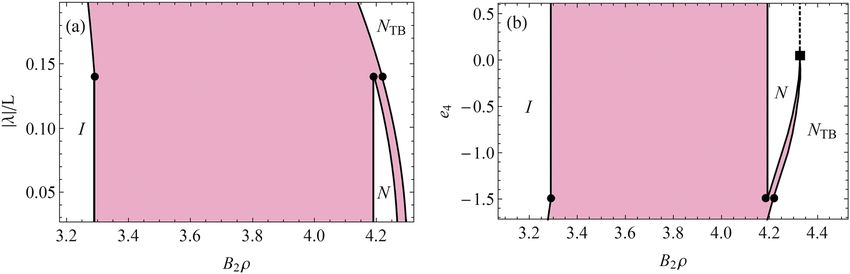
Finally, we map out two phase diagrams of Figs. 7(a) and 7(b).
In Fig. 7(a), we plot the phase diagram as a function of the particle
concentration c = B2 ρ and the modulus of the flexoelectric coupling
coefficient |λ| for the same coefficients as above, i.e., e2 = 1, S0 = 0.85,
e4 = −1, κ = 0.1L2 , and e6 = 10. The pink regions represent two-phase
coexistence regions. At |λ| < 0.14L, the phase diagram features the
“Onsager”-type first-order I–N transition followed by a weakly first-
order N–N TB transition at higher densities. At |λ| > 0.14L, however,
we find a direct first-order I–N TB transition of which the coexist-
ing densities decrease with an increase in |λ|. The two regimes are
separated by an I–N–N TB triple point at |λ| = 0.14L. It is important
to observe that the I–N TB transition remains always first-order such
that we never find a second-order I–N TB transition. Moreover, at λ
= 0, a first-order phase transition is found from a uniaxial N phase
to an N TB phase with an infinite pitch, i.e., a polar nematic phase. In
Fig. 7(b), instead, we build a phase diagram as a function of parti-
cle concentration c = B2 ρ and coefficient e4 of the |P|4 term that we
allow to be negative because of the presence of a stabilizing (positive)
|P|6 term in the grand potential. We fix the other coefficients to the
values as employed above, i.e., e2 = 1, λ = 0.08L, κ = 0.1L2 , e6 = 10,
and S0 = 0.85. Again, the pink regions represent bulk coexistence
regions. We note that we have chosen a value of λ such that the I–N
transition is followed by an N–N TB transition at e4 = −1 according
to Fig. 7(a). For −1.5 < e4 < 0, we find the “Onsager”-type first-order
I–N transition followed by a weakly first-order N–N TB transition.
We observe, however, a direct strongly first-order I–N TB transition
for e4 < −1.5 and an I–N–N TB triple point at e4 = −1.5. Furthermore,
we find that the line of first-order N–N TB transitions ends in a tri-
critical point at (c = 4.3, e4 = 0). At e4 > 0, the N–N TB transition
ceases to be first-order and becomes second-order as illustrated by
the dashed line.
As a final observation, we mention that the formalism intro-
duced in this section should also hold for the N SB phase. Despite
reasonable efforts, but not exhaustive, we did not find a set of coef-
ficients for which the N SB phase is more stable than the N TB one.
FIG. 6. Scalar nematic order parameter (brown and blue) and amplitude of the However, since in simulations and Onsager theory only an N–N TB
polarity P (black) as a function of the particle concentration c = B2 ρ for the coeffi-
phase transition was found, we focused on the latter one. Very inter-
cients e2 = 1, λ = 0.08L, κ = 0.1L2 , e6 = 10, S0 = 0.85, and e4 = −1 (a) or e4 = 1
(b). The equilibrium q and θ are represented in orange and violet, respectively. In
estingly, the nematic spinodal of such a putative N–N SB transition
(a), the “Onsager”-type first-order I–N transition with coexisting concentrations cI would coincide with the nematic spinodal of the N–N TB phase found
= 3.290 and cN = 4.191 is followed by a weakly first-order N–NTB transition with here. Furthermore, by breaking the degeneracy between K 11 and
coexisting concentrations cN = 4.265 and cNTB = 4.295, i.e., a density jump on K 33 , i.e., by setting l3 ≠ 0 in Eq. (3), the first-order N–N TB phase
the order of 1%. The inset shows a zoomed-in view of the discontinuous jump transition described in this section could be followed by a first-order
in the scalar order parameter at the N–NTB transition. In (b), the “Onsager”-type N TB –N SB phase transition.
first-order I–N transition is instead followed by a continuous second-order N–NTB
transition at cN = cNTB = 4.36.
VI. RENORMALIZED ELASTIC CONSTANTS
The flexoelectric coupling term −λPα ∂ β Qβα of Eq. (6) affects
in Sec. III, followed by a weakly first-order N–N TB phase transition the elastic response of polar nematic phases, which translates into
at βμNNTB = 5.293, where the nematic order parameter jumps from renormalized elastic constants. In order to quantify the renormaliza-
SN = 0.814 to SNTB = 0.836. The coexisting densities are cN = 4.265 tion of the elastic constants, we follow the procedure of Refs. 1 and
and cNTB = 4.295, i.e., a density jump on the order of 1%. Interest- 6. First, we solve the Euler–Lagrange equation ∂(βB2 ωP )/∂Pρ = 0.
ingly, we also find jumps in P, θ, q, and SN cos θ, which is to be con- By using Eq. (4) for the tensor order parameter Q, the fact that P
trasted with a second-order N–N TB phase transition. For instance, and n̂ are perpendicular, i.e., Pα nα = 0, and the fact that Pα Pα = 0 in
upon increasing the chemical potential μ for the parameter e4 = 1, the uniaxial N phase, we find
we find an “Onsager”-type I–N phase transition and subsequently a
second-order N–N TB transition at βμNNTB = 5.36, where SN (μNNTB )
= SNTB (μNNTB ) = 0.847, cN = cNTB = 4.36, and P = θ = q = 0, λS0
Pρ = ∂γ Qργ , (30)
so no jumps at all. 2e2 (S0 − S)
J. Chem. Phys. 152, 224502 (2020); doi: 10.1063/5.0008936 152, 224502-9
Published under license by AIP PublishingThe Journal
ARTICLE scitation.org/journal/jcp
of Chemical Physics
FIG. 7. (a) Phase diagram as a function of the particle concentration c = B2 ρ and the modulus of the flexoelectric coupling coefficient |λ|/L for the coefficients e2 = 1, S0 = 0.85,
e4 = −1, κ = 0.1L2 , and e6 = 10. For a weak flexoelectric coupling (|λ| < 0.14L), an “Onsager”-type first-order I–N transition is followed by a weakly first-order N–NTB transition,
while for strong coupling (|λ| > 0.14L), a direct strongly first-order I–NTB transition occurs. A I–N–NTB triple point stabilizes at |λ| = 0.14L. (b) Phase diagram as a function
of the particle concentration c = B2 ρ and the coefficient e4 for the coefficients e2 = 1, λ = 0.08L, κ = 0.1L2 , e6 = 10, and S0 = 0.85. For −1.5 < e4 < 0, the “Onsager”-type
first-order I–N transition is followed by a weakly first-order N–NTB phase transition, while a strongly first-order I–NTB transition occurs for e4 < −1.5. A I–N–NTB triple point
stabilizes at e4 = −1.5. The line of first-order N–NTB transitions ends in a tricritical point (c = 4.3, e4 = 0), from where it continues as a second-order N–NTB transition. In (a)
and (b), the circles indicate triple points, the square indicates the tricritical point, the pink regions represent coexistence regions, and the dashed line indicates a second-order
transition.
eff eff eff
which upon insertion into Eq. (6), with l3 = 0 for convenience, yields (K11 ), twist (K22 ), and bend (K33 ) elastic constants
λ2 S0 (S0 − 2S) eff 8S2 S0 − 4S
βB2 ωP = − (∂γ Qγα )(∂β Qβα ) βDK11 = βDK11 − ξ(S),
4e2 (S0 − S)2 πL2 S0 − S
eff
λ2 S0 βDK22 = βDK22 , (34)
+ (∂γ Qγα )Qαβ (∂ξ Qξβ ). (31) 2
2e2 (S0 − S)2 eff 8S
βDK33 = βDK33 − ξ(S),
πL2
In the final step, we neglected the terms e4 Pα Pα Pβ Pβ , κ(∂ α Pβ )(∂ α Pβ )
and e6 Pα Pα Pβ Pβ Pγ Pγ in Eq. (6) because they do not contribute to the where K 11 , K 22 , and K 33 are the bare splay, twist, and bend elas-
linear elasticity as they contain derivatives of the nematic director tic constants discussed in Sec. II. Equation (34) directly reveals the
of order higher than two. It follows that the form of the renormal- flexoelectric coupling as the source of the renormalization, since
ized elastic constant is the same for second-order transitions (e4 > 0, λ = 0 gives ξ(S) = 0 and hence no renormalization at all. For λ ≠ 0,
e6 ≥ 0) as well as for first-order ones (e4 < 0, e6 > 0). Using that we observe, however, that the renormalization procedure breaks
ni (∂ j ni ) = (∂ j ni )ni = 0 and that the degeneracy between the renormalized splay and bend elastic
constants, so even though K 11 = K 33 , we have nevertheless that
eff eff
(∂α nβ )(∂α nβ ) = (∇ ⋅ n̂)2 + [n̂ ⋅ (∇ × n̂)]2 + ∣n̂ × (∇ × n̂)∣2 K11 ≠ K33 . The renormalization does not affect the twist elastic con-
eff eff eff
stant, for which K22 = K22 . The elastic constants K11 , K22 = K22 and
− ∇ ⋅ [n̂(∇ ⋅ n̂) + n̂ × (∇ × n̂)], (32)
K 11 = K 33 increase monotonically with S, while the renormalized
eff
we find bend elastic constant K33 starts to decrease beyond a certain value
of S until it becomes zero at Sc = S0 (1 − 9λ2 /(8e2 (2l1 + l2 ))). As dis-
1 S0 − 4S cussed in Secs. IV and V, the second-order N–N TB phase transition
βB2 (ωe + ωP ) = [l1 + l2 − ξ(S)]S2 (∇ ⋅ n̂)2
2 S0 − S occurs at a nematic order parameter value Sc , whereas in the case
1 of a first-order transition, the spinodal of the N phase with respect
+ [l1 + l2 − ξ(S)]S2 ∣n̂ × (∇ × n̂)∣2
2 to the N SB phase is located at Sc . As a consequence, our result is in
1 10S − 3S0 agreement with Selinger’s one in the case of a second-order N–N TB
+ [2l2 + ξ(S)]S(∇ ⋅ n̂)(∇S ⋅ n̂) transition, while in the case of a first-order transition, we find that
3 S0 − S eff
1 S0 − 3S 1 at the transition point, both K 33 > 0 and K33 > 0. In the latter case,
+ [ l2 − ξ(S)](∇S ⋅ n̂)2 + [ l2 − ξ(S)]∣∇S∣2 eff
K33 becomes zero at the nematic spinodal. The bare and the renor-
6 S0 − S 3
malized elastic constants are plotted as a function of the scalar order
+ l1 S2 {[n̂ ⋅ (∇ × n̂)]2 − ∇ ⋅ [n̂(∇ ⋅ n̂) + n̂ × (∇ × n̂)]}, parameter S in Fig. 8 for the coefficients e2 = 1, S0 = 1, λ = 0.08L, and
eff eff
(33) e6 = 10. The monotonic increase in K11 , K22 = K22 and K 11 = K 33
eff
with S, together with the simultaneous softening of K33 , can be
with ξ(S) = 9λ2 S0 /(16e2 (S0 − S)). Comparing Eq. (33) with the observed in Fig. 8. The picture is qualitatively the same for l3 ≠ 0,
eff
Oseen–Frank elastic energy (5) gives us the renormalized splay with K33 vanishing at Sc as given by Eq. (26).
J. Chem. Phys. 152, 224502 (2020); doi: 10.1063/5.0008936 152, 224502-10
Published under license by AIP PublishingThe Journal
ARTICLE scitation.org/journal/jcp
of Chemical Physics
that can be used as guidelines for experiments, simulations, and
microscopic theories. In addition, we have focused on the first-order
N–N TB phase transition. Our model is able to reproduce the discon-
tinuous jumps associated with this transition, including the density
jump and the discontinuities in the polarization and nematic order.
Moreover, in contrast to the case of a second-order N–N TB phase
transition where the bend elastic constant K 33 is positive while its
eff eff
renormalized version K33 vanishes, we have found that K33 vanishes
at the nematic spinodal in the case of a first-order N–N TB transi-
eff
tion so that K 33 and K33 remain positive at the actual transition
point. This finding appears to be general and could help in under-
standing the problem of the softening of the elastic constants in
systems with spontaneous polar order and of the mechanism driv-
ing the onset of the spatially modulated phases in bent-core liquid
crystals.
Finally, it is interesting to employ the LdG theory to study con-
FIG. 8. Bare (K11 , K22 , K33 ) and renormalized (K11 eff eff
, K22 eff
, K33 ) splay, twist, and
bend elastic constants as a function of the scalar nematic order parameter S
finement effects of these spatially modulated nematic phases and to
for the fixed values of the coefficients e2 = 1, S0 = 1, λ = 0.08L, and e6 = 10. investigate the structure of the interface between a coexisting N TB
While K11 eff
, K11 = K33 , and K22 eff
= K22 increase monotonically with S, K33 eff and an N SB phase with either an isotropic, uniaxial nematic or a
starts to decrease beyond a certain value of S, until it becomes zero at S = S0 (1 substrate. We will postpone this to future work.
− 9λ2 /(8e2 (2l 1 + l 2 ))). This nematic order parameter value Sc is where the N–NTB
transition occurs if it is second-order, while it is the spinodal S∗ of the N phase with
respect to the NTB one in the case of a first-order N–NTB transition. S+ indicates
the spinodal of the NTB phase with respect to the uniaxial N one.
ACKNOWLEDGMENTS
The authors acknowledge help by S. Paliwal with the numeri-
cal calculations and by A. Grau Carbonell in the realization of Fig. 1.
They acknowledge financial support from the “Nederlandse Organ-
isatie voor Wetenschappelijk Onderzoek” (NWO) TOPPUNT. This
VII. CONCLUSIONS AND DISCUSSION work was part of the D-ITP consortium, a program of the NWO that
is funded by the Dutch Ministry of Education, Culture and Science
In this paper, we have developed a phenomenological LdG the- (OCW).
ory for lyotropic suspensions of bent hard rods, using a Q-tensor
expansion of the chemical-potential dependent grand potential. In
addition, we introduce a bend flexoelectric term that couples the
polarization and the divergence of the Q-tensor to study the stabil- APPENDIX: GRAND POTENTIAL DENSITY OF THE N TB
ity of uniaxial (N), twist-bend (N TB ), and splay-bend (N SB ) nematic AND N SB PHASES FOR l 3 ≠ 0.
phases of colloidal bent rods as a function of particle concentration. In order to compute the grand potential density of the N TB
We first showed that our LdG theory can be mapped onto an Oseen– phase, we insert n̂TB = (sin θ cos(qz), sin θ sin(qz), cos θ) in the ten-
Frank theory. Subsequently, by breaking the degeneracy between sor order parameter Qαβ (r) = 23 S(r)(nα (r)nβ (r) − 31 δαβ ) and the
the splay and bend elastic constants, we find that the LdG theory resulting Q, together with PTB = (P sin(qz), −P cos(qz), 0), in the
predicts either an N–N TB –N SB or an N–N SB –N TB phase sequence grand potential given by Eq. (1). We minimize the obtained grand
upon increasing the particle concentration. We have mapped out potential with respect to the wave number q and the tilt angle θ,
several phase diagrams as a function of the particle concentration respectively, and find
3λ sin(2θTB )SP
qTB = 2 4 2 4
(A1)
8κP2 + 4S2 (2l 2 3
1 + l2 ) sin θTB − 4l2 S sin θTB + 2S l3 (sin θTB − sin θTB )
and
√
2 κP2 κP2 (κP2 + S2 l1 )
sin θTB = 2 + . (A2)
S l1 S2 l1
J. Chem. Phys. 152, 224502 (2020); doi: 10.1063/5.0008936 152, 224502-11
Published under license by AIP PublishingYou can also read