QCD at finite temperature and chemical potential from Dyson-Schwinger equations
←
→
Page content transcription
If your browser does not render page correctly, please read the page content below
QCD at finite temperature and chemical potential from Dyson-Schwinger equations

                                                                                                    Christian S. Fischera,b,1
                                                                  a
                                                                      Institut für Theoretische Physik, Justus-Liebig–Universität Giessen, 35392 Giessen, Germany
                                                                                             b
                                                                                               HIC for FAIR Giessen, 35392 Giessen, Germany

                                          Abstract
                                          We review results for the phase diagram of QCD, the properties of quarks and gluons and the resulting proper-
                                          ties of strongly interacting matter at finite temperature and chemical potential. The interplay of two different
                                          but related transitions in QCD, chiral symmetry restoration and deconfinement, leads to a rich phenomenology
arXiv:1810.12938v2 [hep-ph] 21 Jan 2019

                                          when external parameters such as quark masses, volume, temperature and chemical potential are varied. We
                                          discuss the progress in this field from a theoretical perspective, focusing on non-perturbative QCD as encoded in
                                          the functional approach via Dyson-Schwinger and Bethe-Salpeter equations. We aim at a pedagogical overview
                                          on the physics associated with the structure of this framework and explain connections to other approaches,
                                          in particular with the functional renormalization group and lattice QCD. We discuss various aspects associated
                                          with the variation of the quark masses, assess recent results for the QCD phase diagram including the location
                                          of a putative critical end-point for Nf = 2 + 1 and Nf = 2 + 1 + 1, discuss results for quark spectral functions
                                          and summarise aspects of QCD thermodynamics and fluctuations.
                                          Keywords: QCD phase diagram, Columbia plot, quark-gluon plasma, critical end-point, Dyson-Schwinger
                                          equations

                                             1
                                                 christian.fischer@physik.uni-giessen.de

                                          Preprint submitted to Progress in Particle and Nuclear Physics                                                            January 23, 2019
Contents

1 Introduction                                                                                                                                    3

2 Generalities                                                                                                                                    5
  2.1 QCD phase diagram . . . . . . . . . . . . . . . . . . . . . . . . . .      .   .   .   .   .   .   .   .   .   .   .   .   .   .   .   .    5
      2.1.1 A sketch . . . . . . . . . . . . . . . . . . . . . . . . . . . . .   .   .   .   .   .   .   .   .   .   .   .   .   .   .   .   .    5
      2.1.2 More structure and additional axis’ . . . . . . . . . . . . . .      .   .   .   .   .   .   .   .   .   .   .   .   .   .   .   .    6
      2.1.3 Curvature of the phase boundary . . . . . . . . . . . . . . .        .   .   .   .   .   .   .   .   .   .   .   .   .   .   .   .    8
      2.1.4 Detecting the critical end point by observables: fluctuations        .   .   .   .   .   .   .   .   .   .   .   .   .   .   .   .    9
  2.2 The Columbia plot . . . . . . . . . . . . . . . . . . . . . . . . . . .    .   .   .   .   .   .   .   .   .   .   .   .   .   .   .   .   11
      2.2.1 A sketch . . . . . . . . . . . . . . . . . . . . . . . . . . . . .   .   .   .   .   .   .   .   .   .   .   .   .   .   .   .   .   11
      2.2.2 Extension to real and imaginary chemical potential . . . . .         .   .   .   .   .   .   .   .   .   .   .   .   .   .   .   .   12

3 Non-perturbative quark and glue                                                                                                                15
  3.1 Functional equations . . . . . . . . . . . . . . . . . . . . . . . . . . . . . . . . . . . . . . . .                               .   .   15
  3.2 Quarks, gluons and order parameters . . . . . . . . . . . . . . . . . . . . . . . . . . . . . . .                                  .   .   17
      3.2.1 Chiral transition . . . . . . . . . . . . . . . . . . . . . . . . . . . . . . . . . . . . . .                                .   .   18
      3.2.2 Deconfinement transition . . . . . . . . . . . . . . . . . . . . . . . . . . . . . . . . .                                   .   .   19
      3.2.3 Positivity and spectral functions . . . . . . . . . . . . . . . . . . . . . . . . . . . . . .                                .   .   22
  3.3 Truncation strategies . . . . . . . . . . . . . . . . . . . . . . . . . . . . . . . . . . . . . . . .                              .   .   24
      3.3.1 General considerations . . . . . . . . . . . . . . . . . . . . . . . . . . . . . . . . . . .                                 .   .   24
      3.3.2 Exploring the Columbia plot: a truncation including the Yang-Mills sector explicitly .                                       .   .   27
      3.3.3 Rainbow-ladder and beyond rainbow-ladder truncations using a model for the gluon                                             .   .   29
  3.4 Brief overview on selected vacuum results: gluons and quarks . . . . . . . . . . . . . . . . .                                     .   .   30
      3.4.1 The gluon . . . . . . . . . . . . . . . . . . . . . . . . . . . . . . . . . . . . . . . . . .                                .   .   30
      3.4.2 The quark . . . . . . . . . . . . . . . . . . . . . . . . . . . . . . . . . . . . . . . . . .                                .   .   33
  3.5 Brief overview on selected vacuum results: mesons and baryons . . . . . . . . . . . . . . . .                                      .   .   35
      3.5.1 Mesons . . . . . . . . . . . . . . . . . . . . . . . . . . . . . . . . . . . . . . . . . . .                                 .   .   35
      3.5.2 Baryons . . . . . . . . . . . . . . . . . . . . . . . . . . . . . . . . . . . . . . . . . . .                                .   .   37

4 Results under variation of the number and masses of quarks, temperature and chemical potential                                                 39
  4.1 Heavy quark limit: (De-)confinement and the Roberge-Weiss transition . . . . . . . . . . . . . .                                           39
      4.1.1 Pure gauge gluon propagator at finite temperature . . . . . . . . . . . . . . . . . . . . .                                          39
      4.1.2 Phase structure of QCD for heavy quarks . . . . . . . . . . . . . . . . . . . . . . . . . . .                                        42
  4.2 Nf = 2: Critical scaling in the chiral limit and temperature dependence of meson masses . . . .                                            44
  4.3 Physical quark masses: The critical end point for Nf = 2 + 1 and Nf = 2 + 1 + 1 . . . . . . . . .                                          48
      4.3.1 The QCD phase diagram for Nf = 2 + 1 . . . . . . . . . . . . . . . . . . . . . . . . . . .                                           48
      4.3.2 The QCD phase diagram for Nf = 2 + 1 + 1 . . . . . . . . . . . . . . . . . . . . . . . . .                                           51
      4.3.3 Baryon effects on the CEP . . . . . . . . . . . . . . . . . . . . . . . . . . . . . . . . . . .                                      52
  4.4 Thermodynamics and quark number susceptibilities . . . . . . . . . . . . . . . . . . . . . . . . .                                         54
  4.5 Quark spectral functions and positivity restoration . . . . . . . . . . . . . . . . . . . . . . . . .                                      56
  4.6 Colour superconductivity . . . . . . . . . . . . . . . . . . . . . . . . . . . . . . . . . . . . . . . .                                   59

5 Outlook                                                                                                                                        62

 A                  Multiplicative renormalizability in the DSEs for the propagators                                                             63
1   Introduction
Exploring the structure of the phase diagram of QCD, unravelling the potential existence of a critical end point
(CEP) and mapping out the region of a first order transition at large chemical potential are major goals of
current and future experimental programs at the Relativistic Heavy Ion Collider (RHIC) at the Brookhaven
National Laboratory (BNL) and future experiments at the FAIR facility in Darmstadt and NICA in Dubna. These
experiments seek to probe the chiral as well as the deconfinement transition from the hadronic state of mat-
ter to the quark-gluon plasma phase. The experimental verification of a CEP would be a major step in our
understanding of QCD and an important cornerstone in the further exploration of the QCD phase diagram.
    Non-perturbative methods are mandatory in this endeavour. Lattice QCD has firmly established the notion
of an analytic crossover at zero chemical potential [1–6]. However, the situation is much less clear at (real)
chemical potential, where lattice calculations are hampered by the notorious fermion sign problem. Although
much progress has been made in the past years it seems fair to say that a satisfactory solution of this problem
is yet to be found. Various extrapolation methods from zero or imaginary chemical potential into the real
chemical potential region have been explored and agree with each other for chemical potentials µB /T < 2.
Then errors accumulate rapidly and solid predictions are not yet possible.
    Larger chemical potentials are accessible by continuum methods, i.e. effective models and the functional
approach. The Polyakov-loop enhanced effective models such as the Polyakov-loop Nambu–Jona-Lasinio model
(PNJL) [7–9] and the Polyakov-loop quark-meson model (PQM) [10–12] are excellent tools to study a range of
fundamental and phenomenological questions related to the QCD phase diagram, see e.g. [13, 14] for recent
review articles and comprehensive guides to the literature. These models rely on a chiral effective action
augmented by the Polyakov loop potential which serves as a background that couples the physics of the Yang-
Mills theory (in particular its confining aspects) to the chiral dynamics. However, gluons are no active degrees
of freedom and their reaction to the medium can neither be studied nor directly taken into account.
    This is possible within functional approaches to QCD. Dyson-Schwinger equations, the functional renormal-
isation group, the Hamilton variational approach and the Gribov-Zwanziger formalism work with the quark
and gluon degrees of freedom and determine the phase structure of QCD from order parameters extracted
from Green’s functions. In general, the functional approach is restricted by the need to truncate an infinite
system of equations to a level which can be dealt with numerically. The truncation assumptions, however, are
not arbitrary and can be systematically assessed. Consequently, in the past decade functional methods have
contributed substantially to our understanding of the phase diagram, the properties of quarks and gluons and
observable consequences related to thermodynamics, transport and fluctuations.
    Certainly, a review of this size cannot be complete and we selected the material reflecting our personal
interest. We focus a choice of topics that has been addressed via the framework of Dyson-Schwinger (DSE)
and Bethe-Salpeter (BSE) equations and reflect the progress that has been made in the almost twenty years
since the renowned review of Roberts and Schmidt [15]. Whenever appropriate, we will also make contact
with results obtained using other functional approaches and provide links to results from lattice gauge theory.
Nevertheless, it is clear that many equally interesting topics cannot be properly done justice to the given amount
of space and time.
    We start the discussion in section 2 with general remarks on the QCD phase diagram, possible phases in the
temperature and real chemical potential plane and comments on interesting extensions into several directions
such as imaginary chemical potential, isospin chemical potential or non-zero magnetic field. We focus in some
detail on the physics of the Columbia plot of non-physical quark masses and highlight the interesting interplay
of chiral and deconfinement transitions in various limits. In section 3 we summarise the DSE approach and
discuss truncation strategies. A brief overview on selected results in the vacuum serves as a basis for the
subsequent presentation of results at finite temperature and chemical potential in section 4. We walk through
the Columbia plot starting with the pure gauge corner and the region of first and second order deconfinement
transitions in section 4.1, spend some time in the upper left corner of a potential second order chiral transition
in section 4.2 and then concentrate on results for physical quark masses in section 4.3. In section 4.4 we
summarise results on observable quantities related to thermodynamics and fluctuations and discuss the issue
of quark spectral functions and positivity in section 4.5. We then conclude the section with a brief overview on
DSE-results for the color superconducting region of the QCD phase diagram 4.6. A general outlook is given in

                                                        3
section 5. Some technical details are relegated to an appendix.
    Readers mostly interested in the context of the research field and the results and solutions offered by the
functional approach are encouraged to skip section 3 in a first reading and directly progress from section 2 to
section 4. In a second reading the technical details and general considerations on DSEs offered in section 3
may then be beneficial.

                                                      4
200

                                                   Crossover
                                         150
                                                                              ?

                     Temperature [MeV]
                                                      Critical Endpoint
                                                                                      First Order Phase Transition
                                         100

                                          50
                                                                                              ?
                                                                                                    Color Superconducting
                                                           Nuclear Liquid-Gas Transition            Phases

                                           0
                                               0     200       400      600           800    1000        1200      1400
                                                                 Baryon chemical potential [MeV]

             Figure 2.1: Sketch of the QCD phase diagram in the temperature and baryon chemical potential plane.

2     Generalities
2.1     QCD phase diagram
2.1.1    A sketch
Even after decades of theoretical and experimental exploration, the sketch of the QCD phase diagram given
in Fig. 2.1 is largely driven by (more or less well-grounded) speculation. There is widespread agreement
that results from lattice QCD [1–6] demonstrate an analytic cross-over at zero chemical potential from a
low-temperature phase characterised by confinement and chiral symmetry breaking to a high-temperature
deconfined and (partially) chirally restored phase where the quark-gluon plasma (QGP) is realized. The cor-
responding pseudo-critical temperature for the chiral transition has been localized at Tc ≈ 155 MeV with an
error margin below ten MeV [3, 4]. Furthermore, the thermodynamic properties of the hot matter in a broad
temperature range around Tc have been pinned down with great accuracy [6, 16–19] and serve as input and
benchmark for a large number of phenomenological applications. Thus the emerging standard picture of the
situation at zero baryon chemical potential µB and physical quark masses is that of a continuous cross-over
characterized by narrow but finite peaks in various susceptibilities.
    Many model calculations suggest, that this continuous cross-over becomes steeper with increasing chemical
potential and finally merges into a second-order order critical end-point (CEP) followed by a region of first-
order phase transition at large chemical potential [20–22]. In Ref. [23] one of the main arguments for the
existence of such a critical end-point has been formulated accordingly: (i) we know that there is an analytic
cross-over at finite temperature and zero chemical potential; (ii) we believe (from model studies) that the
chiral phase-transition along the zero temperature and finite chemical potential axis is first-order. It is then
highly suggestive (if not thermodynamically unavoidable) that there has to be a critical end-point somewhere
in the QCD phase diagram. Another argument along similar lines even suggests the universality class of the CEP
[21, 24, 25]: From symmetry arguments (cf. the discussion in section 2.2 below) one is led to believe that the
T -µB -phase diagram of the two-flavour theory in the chiral limit features a line of second order phase transition
points that merges into a tricritical point followed by a region of first order transition at large chemical potential
- similar to the sketch of Fig. 2.1 but with cross-over replaced by second order and critical endpoint replaced by
tricritical point. This second order line is expected to be in the universality class of O(4) spin models in three
dimensions [26] with three pseudoscalar pion fields and one scalar sigma field as massless degrees of freedom.
In the theory with massive quarks (Fig. 2.1) the second order line collapses into a single second order point (the

                                                                                  5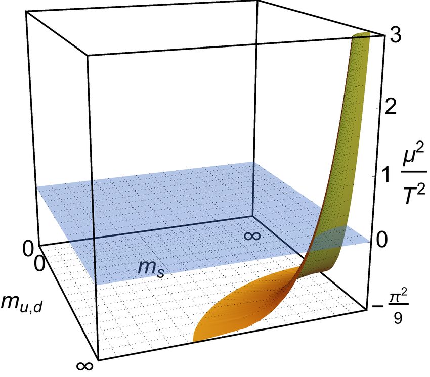
CEP), and the pion fields are no longer Goldstone bosons but become massive. The remaining massless sigma
field at the CEP places the theory then in the Z(2) universality class of the Ising model in three dimensions2 .
    In principle, there are at least two obvious strategies to make these suggestions more rigorous: first, one
could follow the cross-over line into the phase diagram until one hits the critical end-point and second, one
could aim to nail down the first-order nature of the phase-transition at zero temperature and large chemical
potential. The first strategy has been followed by lattice QCD and functional methods. In general, lattice
calculations suffer from the notorious sign-problem at finite chemical potential and therefore need to involve
extrapolations from zero to positive real chemical potential. Methods like Taylor expansion, re-weighting
schemes or extrapolation from imaginary chemical potential (where the sign problem is not present) thus
allow for indirect access to quantities at moderate chemical potential [28–31]. These methods have been
refined over the years and work well up to the region of µB /T . 2 [19, 32], after which errors accumulate
rapidly. In contrast to early lattice studies [33–35] which indicated the presence of a critical end-point at rather
small chemical potentials, there seems to be agreement from recent studies that a potential CEP may only be
located in the region µB /T > 2 [19, 32]. As we will see in the course of this review, this finding is in agreement
with the ones from Dyson-Schwinger studies [36, 37].
    The second strategy, aiming at clarifying the situation at zero (or small) temperature and large chemical
potential is hampered by the potentially rich physics in this region of the QCD phase diagram. It is probably fair
to say, that there is currently no approach that captures all features of this physics and therefore to quite some
degree this is the realm of speculation, based on more or less rigorous studies. For zero temperature and small
chemical potential, a well-founded expectation is the silver-blaze property of QCD: unless the baryon chemical
potential is larger than the lowest baryon mass in medium (i.e. roughly the mass of the nucleon minus 16 MeV
binding energy), the system must stay in the vacuum ground state and all observable quantities are similar to
the vacuum. In the QCD path integral formulation, this property can be shown analytically for the case of finite
isospin chemical potential, but on physical grounds it is at least extremely plausible also for the case of finite
baryon chemical potential [38, 39]. In a lattice calculation with heavy but dynamical quarks the silver blaze
property of QCD has been demonstrated in Ref. [40]. In the Dyson-Schwinger framework suitable truncations
that respect the silver blaze problem are discussed in [41].
    As soon as the chemical potential reaches values beyond the silver blaze region the system is able to produce
baryonic matter. In model calculations (see e.g. [13, 42] for overviews) this is associated with a first-order
phase transition which can be identified with the liquid-gas transition of infinite nuclear matter. The associated
order parameter is the baryon density, which jumps from zero to ρ0 = 0.17/fm3 . Signals for this transition have
again been observed in an effective lattice theory [43] and are also visible in contemporary chiral mirror meson-
baryon models [44]. At even larger chemical potential, model studies find the above mentioned first-order
chiral transition, which in sufficiently rich models progresses directly into a (number of) color superconducting
phase(s), see e.g. [25, 45–52]. In the Dyson-Schwinger approach, superconducting phases have been studied
in [41, 53–57] with the aim to clarify the interplay between the superconducting 2SC phase (only up- and
down-quarks form Cooper pairs) and the color-flavor-locked (CFL) phase (up- down- and strange-quarks are
paired symmetrically). We will discuss this topic in more detail in section 4.6. It is probably worth mentioning,
that in principle there could be a gap between the phases with broken chiral symmetry and the one with colour
superconductivity. There has been some debate about this possibility in the context of QED3 as an effective
model for high temperature superconductors, see e.g. Refs. [58–61]. In this context the gap is generated by a
region with chirally restored but non-superconducting matter. There are, however, other possibilities as will be
summarised in the next subsection.

2.1.2    More structure and additional axis’
So far we discussed the sketch in Fig. 2.1, but there is much more. An important possibility, well-known in
solid state physics, has been suggested for QCD in [62–65] and reviewed in [66]. It is the appearance of an
inhomogeneous phase, where the quark condensate is spatially modulated at moderate temperatures and high

   2
     This picture including the O(4) and Z(2) scaling behaviour has been confirmed in renormalization group studies of the PQM model
[27].

                                                                 6
densities. In the sketch of 2.1 this corresponds to the region where the putative first order chiral transition
between the hadronic and the quark-gluon plasma or color superconducting phases takes place. Investigations
using Ginzburg-Landau theory, effective models (NJL, QM, PQM), large Nc expansions or Dyson-Schwinger
techniques indicate, that this possibility has to be taken seriously. However, most of these studies are only
performed on the mean field level. Since it is known that fluctuations may have a significant influence on the
phase structure of a theory, no firm conclusions can be made so far. A beyond mean field treatment has been
performed within the framework of Dyson-Schwinger equations in Ref. [67], with a chiral-density-wave like
modulation of the condensate taken into account in the quark-sector of QCD (but not in closed quark loops).
One of the striking results of this calculation (in agreement with effective model approaches; see however [68]
for counterexamples) is the appearance of the inhomogeneous phase precisely at and around the first order
transition with a so called Lifshitz point3 at the location of the critical end point. We will briefly come back to
this result in section 4.3. It is an important task for the future to corroborate (or reject) the existence of such
inhomogeneous phases in more stringent approaches, in particular with respect to their potential significance
for signals in heavy ion experiments.
    Another possibility, introduced in Ref. [69] and reviewed in Ref. [42] is the appearance of a phase of
’quarkyonic matter’ in the same region of the phase diagram as for the inhomogeneous phase(s). Based on
large-Nc considerations, quarkyonic matter has been described as a state of dense, strongly interacting baryons
that has similar thermodynamic properties as quark matter. Its chiral properties are often associated with
inhomogeneous condensates. Within this review, however, we will not cover this topic in any detail and we
refer the interested reader to the literature, see e.g. [42, 69–71] and references therein.
    There are also a number of possibilities to add more axis’ to the sketch in Fig. 2.1. A huge amount of
literature is available that deals with the effects of non-zero magnetic field onto the various transitions discussed
above. Magnetic fields are interesting in connection with important physics applications: (i) in heavy ion-
collisions huge (but short-lived) magnetic fields are created by the nuclei moving rapidly in opposite directions;
(ii) some compact stars, so called magnetars, are characterized by extremely high magnetic fields that may
have a profound impact on the equation of state; (iii) magnetic fields may have played an important role in the
electroweak phase transition of the early universe. Comprehensive reviews on the effects of magnetic field are
e.g. Refs. [72, 73]. From a fundamental point of view, one of the most interesting effects of a non-vanishing
magnetic field is the generation of magnetic catalysis, i.e. the fact that an external magnetic field initiates (or
enhances) the dynamical generation of fermion masses even in theories with only weak interaction [74, 75].
This effect has been studied in detail over the years and similarities and discrepancies with Cooper pairing
effects have been worked out, see [73] for an overview. Perhaps surprisingly, results from lattice QCD also
demonstrate that the opposite effect happens for large enough temperatures: the dynamical mass generation
is reduced and consequently the transition temperatures for the crossover to the chirally restored phase is
decreased [76–80]. This effect, not present in simple models, can be traced back on the back-reaction of the
quarks onto the Yang-Mills sector, and has been seen also in the Dyson-Schwinger framework [81]. A further
interesting consequence of non-vanishing magnetic fields, discussed extensively in the literature, is the chiral
magnetic effect of generated electric currents in heavy ion collisions, see e.g. [82] for a recent review. In this
context the introduction of finite chiral chemical potential µ5 has been considered within lattice QCD [83–86],
effective models [87–90] and the Dyson-Schwinger framework [91–93].
    Another axis that can be added to the sketch in Fig. 2.1 is one of finite isospin chemical potential µI ,
which creates an imbalance between up- and down-quarks [94]. This axis is by no means academic, since this
imbalance is present in heavy ion collisions (due to different numbers of protons and neutron in the colliding
nuclei), as well as in compact stars due to β-equilibrium and charge neutrality. The study of the QCD phase
diagram with zero baryon chemical potential but non-zero µI is furthermore of systematic interest since it
allows comparisons of the results of lattice QCD (which can be simulated at finite µI [95–98]) with studies in
other approaches, see e.g. [99–104] and references therein. The physics of finite isospin chemical potential
is related to several phase transitions. For µI < µπ /2 the silver-blaze phenomenon takes place, similar to the
situation at finite baryon chemical potential. One then finds a second order transition to a phase with pion

   3
     I.e. the point where the inhomogeneous phase, the chirally symmetric and the chirally broken phase meet, c.f. [66] p.20 for a
discussion of the precise terminology.

                                                                7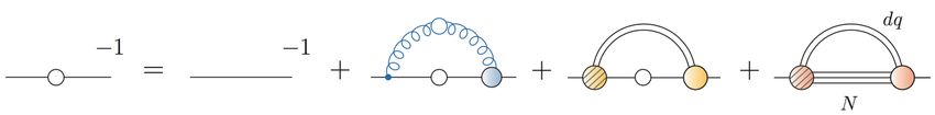
κ
                            200                                                                  Lattice [108]             0.0180 (40)
                                                                                                 Lattice [109]             0.0130 (30)
                            150                                                                  Lattice [110]             0.0135 (20)
        Temperature [MeV]

                                                                                                 Lattice [32]              0.0149 (21)
                            100                                                                  Lattice [111]             0.0145 (25)
                                                                                     QM-model (Nf = 2) [112]                0.0155 (7)
                            50                                                       QM-model (Nf = 2) [113]                0.0157 (1)
                                                                                                                            0.0160 (1)
                                                                                                                            0.0089 (1)
                             0
                              0   200    400 600 800 1000 1200 1400
                                        Baryon chemical potential [MeV]                           DSE [36]                0.0238 (100)

       Figure 2.2: Sketch of the QCD phase diagram - visualisation of the          Table 2.1: Results for the curvature κ of the transi-
       extrapolated curvature range 0.0120 < κ < 0.0141 explained in               tion line from different approaches. The error budget
       the main text.                                                              of the QM-model contains errors from the fitting proce-
                                                                                   dure only; the error of the DSE-result is based on an esti-
                                                                                   mate according to the systematic corrections introduced
                                                                                   in [37]. If not indicated otherwise, all calculations are
                                                                                   performed with Nf = 2 + 1 quark flavours.

condensation, which may even play a role in compact stars, see e.g. [105] and references therein. The pion
condensation phase extends to finite temperature and may show another first order transition accompanied
with a CEP inside [94, 100]. More interesting phenomena (like the appearance of a Fulde-Ferrell-Larkin-
Ovchinnikov (FFLO) phase [94, 106, 107]) occur when both the baryon chemical potential and the isospin
chemical potential are considered.

2.1.3                       Curvature of the phase boundary
Let us now come back to the sketch of Fig. 2.1 and consider again the boundary of the chiral transition in
the region close to vanishing chemical potential. As has been mentioned in the introduction, lattice gauge
theory at non-zero chemical potential is hindered by the sign problem. However, various methods like Taylor
expansion, re-weighting schemes or extrapolation from imaginary chemical potential have been developed
and refined over the years, such that reliable results in the region µB /T . 2 are available. One of the most
interesting issues from an experimental point of view may be the determination of the pseudo-critical line
separating the low-temperature phase from the high-temperature one. At small chemical potential, this line
can be parametrised by an expansion quadratic in the dimensionless ratio of chemical potential to temperature:
                                                                             2                4
                                                     Tc (µB )            µB                 µB
                                                              =1−κ                 −λ                 ··· ,                                 (2.1)
                                                        Tc               Tc                 Tc
with baryon chemical potential µB , pseudo-critical temperature Tc (µB ) and Tc = Tc (0)4 . The expansion is
quadratic, since the grand canonical QCD partition function Z is symmetric with respect to a change of sign in
µB /T [114]                                   µ         µ
                                                 B            B
                                           Z        =Z −          ,                                      (2.2)
                                                T            T
and therefore all odd powers of µB /T in the expansion have to vanish.

   4
    A word of caution is in order here: this expansion has been used in the literature in different forms, sometimes it is formulated
not in baryon but in quark chemical potential and sometimes factors of π 2 are included, resulting in trivial changes of the values of the
expansion coefficients κ and λ. Sometimes on the right hand side Tc (µB ) is used instead of Tc (0). The latter change is immaterial for
small chemical potential but has some impact on extrapolations at larger µB . In this review we will stick to the formulation Eq. (2.1).

                                                                          8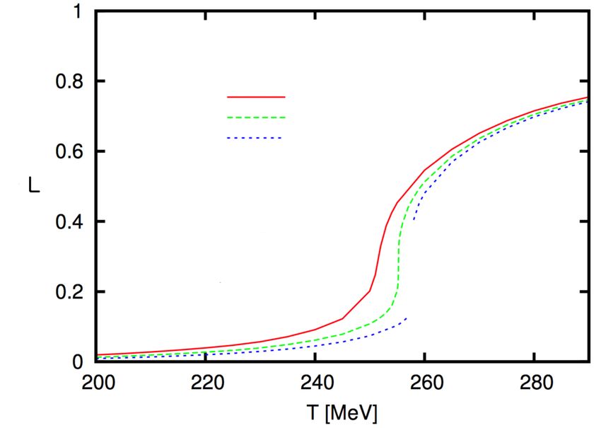
Which values for the curvature κ of the critical transition line can we expect in Eq. (2.1)? Suppose for the
sake of the argument that the sketch of Fig. 2.1 represents the qualitative aspects of the QCD phase diagram
accurately and the chiral transition line is not affected by additional physics in the low-temperature and high
chemical potential region such as inhomogeneous condensates or other phenomena. A naive estimate of κ
can then be based on the following consideration: Because of Eq. (2.2) and analyticity at µB = 0 and T = 0,
the transition lines cross the temperature and chemical potential axis’ perpendicularly.5 A suitable functional
form for the entire transition line including the cross-over and first-order sections that reproduces both, the
quadratic expansion (2.1) around zero chemical potential but also its counterpart for the first order line around
zero temperature is elliptic, i.e.
                                            Tc (µB ) 2
                                                               2
                                                                  µB
                                                       = 1 − 2κ          .                                   (2.3)
                                               Tc                  Tc
The two free parameters are the transition temperature at zero chemical potential Tc ≡ Tc (µB = 0) and the
curvature κ of the transition line. The former is well determined from lattice QCD, Tc ≈ 155 MeV [3, 4]. Using
this value and the safe assumption that the chiral transition at T = 0 cannot happen for chemical potentials
smaller than the liquid-gas transition at µlg
                                           B ≈ 922 MeV we immediately obtain an estimate for the lower bound
of the curvature
                                                   κ ≤ 0.0141 .                                          (2.4)
It is interesting to compare this naive estimate with the results from lattice calculations and continuum ap-
proaches displayed in table 2.1. While earlier lattice studies obtained lower values for the curvature [30, 31,
115], the recent continuum extrapolated results now indicate convergence between different methods (Tay-
lor expansion techniques and analytical continuation from imaginary chemical potential) [32, 108–111]. The
naive estimate of Eq. (2.4) agrees very well with the lattice results. It is also not too far from the results for
the quark-meson model (although this comparison is not rigorous due to differences in Nf ). The DSE-result of
[36] is somewhat larger, although the results of [37] indicate that there is a systematic error that can account
for this discrepancy; this is discussed in detail in sections 4.3.1 and 4.3.3.
     Thus it seems as if our naive estimate is not so bad at all. Indeed, expanding Eq. (2.3) and comparing with
Eq. (2.1) we can also predict the size of the coefficient λ in Eq. (2.1) to be given by
                                                         1
                                                      λ = κ2 ≤ 0.0001 .                                                     (2.5)
                                                         2
This value is very small. Recent lattice estimates indeed confirm that λ may be orders of magnitude smaller
than κ [116, 117], although the error bars are still large.
    Taking the error band of the lattice result in Ref. [111] as a lower limit we arrive at the spread of tran-
sition lines show in Fig. 2.2 representing the range 0.0120 < κ < 0.0141. This construction establishes a
connection between rigorous results at finite temperature and zero chemical potential and the zero tempera-
ture large chemical potential region, and predicts a chiral transition at 922 . µB . 1000 MeV. Of course, this
naive construction may very well be modified by dynamical effects at large chemical potential including the
potential appearance of additional phases such as the inhomogeneous one discussed in the previous section.
Nevertheless, it is amusing to see that this simple procedure leads to intuitive and interesting predictions.

2.1.4    Detecting the critical end point by observables: fluctuations
As mentioned in the introduction, it is one of the main goals of contemporary (Beam Energy Scan program
at RHIC) and future (CBM/FAIR and NICA) experimental programs to study the existence and the location of
the critical end point in the QCD phase diagram. To this end it is vital to identify observables that connect the
theoretical properties of the CEP with experimental data. This endeavour is reviewed extensively in Ref. [118]
and we therefore give only a brief overview here. Provided the chemical freeze-out in heavy ion collisions is
sufficiently close to the chiral critical line and the CEP, it has been suggested [21, 22, 119–123] that fluctuations

   5
    At zero temperature and finite chemical potential this is also guaranteed thermodynamically by the Clausius-Clapeyron relation,
provided the transition is first order.

                                                                9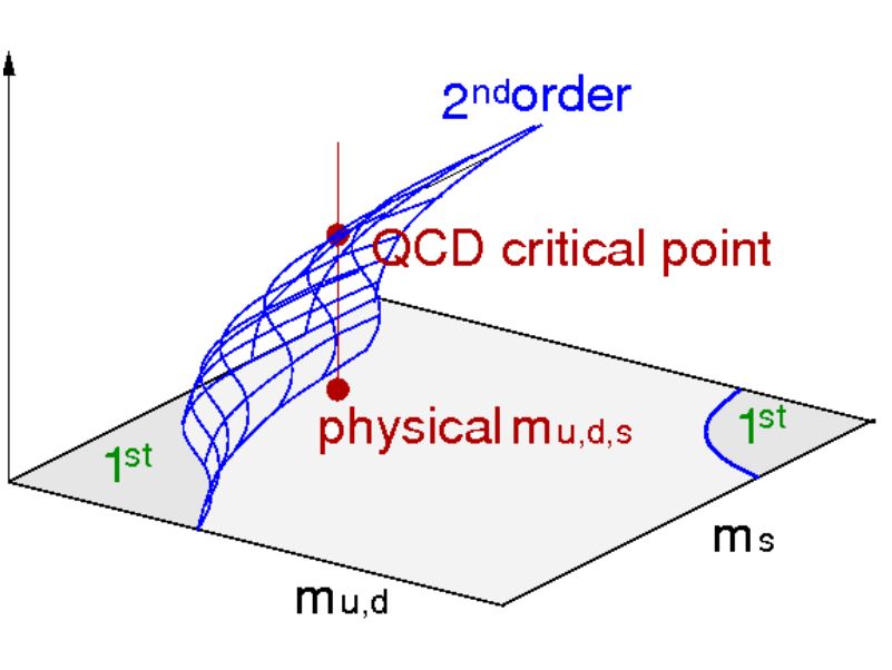
of conserved charges provide important information on the location of the CEP. In the experiments these appear
as event-by-event fluctuations of the net baryon number B, the electric charge Q or the strangeness S of the
heavy ion system. In particular, ratios of susceptibilities are expected to provide clean signals.
    In order to analyse these quantities theoretically one starts from the dimensionless pressure P/T 4 extracted
from the QCD partition function via
                                      P      1
                                         =      ln[Z(V, T, µB , µQ , µS )] ,                               (2.6)
                                      T4   V T3
with Lagrange multipliers for the baryon chemical potential µB , the charge µQ and the strangeness chemical
potential µS . The normalized generalised susceptibilities are defined via

                                                     ∂ l+m+n (p/T 4 )
                                    χBSQ
                                     lmn =                                    .                            (2.7)
                                             ∂(µB /T )l ∂(µS /T )m ∂(µQ /T )n

Experimentally, ratios of cumulants
                                               BSQ
                                              Clmn = V T 3 χBSQ
                                                            lmn                                            (2.8)
are extracted that do not depend explicitly on the volume (though there may be implicit dependencies) and
can be directly compared with ratios of theoretical susceptibilities, see [118] for details. They are related to
statistical quantities via

                                         mean:        MB = C1B ,
                                                        2
                                       variance:       σB = C2B ,
                                      skewness:        SB = C3B /(C2B )3/2 ,
                                       kurtosis:       κB = C4B /(C2B )2 ,                                 (2.9)

for the example of baryon number and analogous expressions for charge and strangeness.
    In terms of quark degrees of freedom, the chemical potentials for baryon number, strangeness and charge
can be related to the chemical potentials of the up, down and strange quarks via

                                           µu = µB /3 + 2µQ /3 ,
                                           µd = µB /3 − µQ /3 ,                                           (2.10)
                                           µs = µB /3 − µQ /3 − µS .

In order to take into account the situation of heavy-ion collisions, these need to be adjusted appropriately.
Strangeness conservation in the colliding nuclei implies that the mean density of strange quarks vanishes,
i.e. hns i = χS1 = 0. On the other hand, typical ratios of the number of baryons to protons in Au-Au and
Pb-Pb collisions imply that hnQ i = Z/A hnB i with Z/A ≈ 0.4. Thus the dependence of µQ and µS on µB
or alternatively µu , µd and µs need to be defined such that these conditions are satisfied. This has been
studied in lattice simulations at small chemical potentials [124, 125]. Within errors both groups agree that for
temperatures around T = 150 MeV the leading order result is µQ ≈ −0.02 µB , while µS ≈ 0.2 µB . Thus to a
good approximation one can choose µu = µd and µs = 0 to explore the QCD phase diagram. For the location
of the CEP this has been checked in the DSE approach [126], cf. also section 4.3.
    Ratios of generalised susceptibilities have been used to extract the freeze-out points from experimental
data from first principles lattice calculations [124, 125] that can be compared with those obtained from the
Hadron Resonance Gas model [127]. Furthermore various higher order fluctuations have been determined
as functions of temperature and chemical potential [128–134]. In model calculations, it has been shown
that these fluctuations are sensitive to the critical end-point, see e.g. [27, 135–137] and references therein.
Important results include the discovery of the smallness of the critical region around the CEP in calculations
using the renormalization group approach [27] and the appearance of different critical exponents depending
on the path across the CEP [135]. Detailed comparisons between the model results and experimental data have
been performed e.g. in [136, 137].

                                                       10
Figure 2.3: Left: Columbia plot of phase transition lines as functions of quark masses including UA (1) anomaly.
Right: Same plot with UA (1) anomaly restored.
2.2 The Columbia plot
2.2.1 A sketch
The sketch of the QCD phase diagram discussed in the last section is, if at all, only valid for ’physical quark
masses’, i.e. quark masses that lead to a physical hadron spectrum in agreement with experiment. From
a theoretical point of view it is also highly interesting to consider situations with unphysical values for the
up-, down- and strange-quark masses. The variation of these reveals the intricate interplay of chiral and
deconfinement transitions, sketched in Fig.(2.3), the ’Columbia plot’ [138]. Each of these transitions is related
to an underlying symmetry of QCD: chiral symmetry and center symmetry. Their explicit breaking due to
non-vanishing (chiral) or non-infinite (center) quark masses generates the pattern displayed in Fig.(2.3).
Let us briefly discuss the various regions in the plot starting from the pure gauge theory limit of infinitely
heavy masses in the upper right corner. In this limit the theory is symmetric with respect to center trans-
formations associated with the center of the gauge group, i.e. Z(3) for SU(3). Whereas center symmetry is
maintained in the low temperature phase, it is broken dynamically at large temperatures. The transition tem-
perature of the associated first-order deconfinement transition [139] is much larger than the pseudo-critical
one at the physical point: for SU(3) it is around Tc ≈ 270 MeV, see e.g. [28], whereas other gauge groups
result in different values [140]. The transition can be traced by center sensitive order parameters such as the
Polyakov-loop (cf. section 3.2). Finite-mass quarks in the fundamental representation of the gauge group fur-
thermore break center symmetry explicitly and turn the first-order transition into a cross-over at light enough
masses. The second order separation line in the upper right corner of the Columbia plot is in the Z(2) univer-
sality class [114, 141] and its location in the u/d-s-quark mass plane has been mapped out by lattice gauge
theory [142–144], effective models [145, 146], the Dyson-Schwinger approach [147] and background field
techniques [148, 149]. We come back to this issue in much more detail in section 4.1.
The low-mass corners of the Columbia plot are governed by the chiral transition. Massless QCD with Nf
quark flavours is invariant under a global flavour symmetry UV (1) × UA (1) × SUV (Nf ) × SUA (Nf ). Whereas
UV (1) is conserved and related to the baryon number, SUV (Nf ) is explicitly broken by differences in the finite
quark masses of the QCD-Lagrangian. The most important properties of the chiral transitions of QCD are
governed by the two axial symmetries UA (1) × SUA (Nf ). Whereas the latter one is broken dynamically at
low temperatures (and always explicitly by finite quark masses), the former one is broken anomalously. The
corresponding current Jµ5 = Ψ̄γµ γ5 Ψ with quark fields Ψ is not conserved,
g 2 Nf
∂ µ Jµ5 = tr F̃µν F µν
, (2.11)
16π 2
due to the appearance of the topological charge density on the right hand side. Both, the dynamical and
11anomalous breaking can be restored at large temperatures, albeit the corresponding transition temperatures
may very well differ from each other, since the underlying physics is different: any temperature effect that
significantly reduces the interaction strength of QCD will lead to the restoration of SUA (Nf ); in order to
restore the chiral UA (1), however, one needs an effect that reduces the topological charge density. Although
both restoration mechanisms may be related, they are not necessarily so.
The fate of the UA (1)-symmetry is expected to affect the order of the chiral SUA (Nf ) transition as shown in
the two versions of the Columbia plot given in Fig. 2.3. With an anomalously broken UA (1) at all temperatures
it has been conjectured that the chiral transition for the two flavour theory (upper left corner of the plot) is
second order and in the universality class of the O(4) theory, whereas with restored UA (1) the transition may
remain first order [26] (right diagram). In both scenarios the chiral three-flavour theory (lower left corner
in both diagrams) is expected to be first order[26], since no three-dimensional SU (Nf ≤ 3) second order
universality class is known [150, 151]. With restored UA (1) the two first order corners are expected to be
connected as shown in the right diagram of Fig. 2.3. The corresponding scenario with broken UA (1) in the left
diagram, however, features a tricritical strange quark mass mtri s where the first order region around the chiral
three-flavour point merges into the second order line connected to the chiral two-flavour point.
It is currently an open question which of these scenarios is realised in QCD. For the theory with three
degenerate flavours, lattice studies seem to support the existence of a first order region in the lower left corner
of the Columbia plot [152–158]. However, the size of the first order region depends strongly on the formulation
of the lattice action and the temporal extend of the lattice and has not yet been determined unambiguously.
Even the possibility that the first order region vanishes in the lattice continuum limit is not yet excluded [151].
The situation in the upper left corner and, related, in the chiral limit of the Nf = 2 + 1-theory with strange
quark mass fixed is also not clear and indications from lattice simulations vary between favouring either of the
two scenarios of Fig. 2.3 [109, 159–166].
Both scenarios of Fig. 2.3 can be also realised in effective low energy QCD models such as the PQM or
PNJL model, see e.g. [167–172] and Refs. therein. In Ref. [172] it has been demonstrated that results
on the Columbia plot from mean field approaches are substantially modified once fluctuations have been in-
cluded using the functional renormalisation group (FRG). Depending on the strength of the t’Hooft interaction
parametrizing the effects of the UA (1)-anomaly one then ends up with a chiral phase structure precisely along
the lines of Fig. 2.3 with small first order regions in both scenarios. First results on the chiral two-flavour
theory are also available for functional FRG and DSE approaches to QCD: while the FRG-approach suggests a
second order transition in the chiral limit [173], it has also been shown how O(4)-scaling might emerge in the
DSE-approach [174]. We will come back to this point in much more detail in section 4.2.
2.2.2 Extension to real and imaginary chemical potential
The Columbia plot sketches the variation of the order of the QCD transitions at zero chemical potential. Possible
scenarios for the extension of the plot by a third axis denoting real or imaginary chemical potential are shown
in Figs. 2.4a and 2.4b. Let us first briefly discuss the extension to real chemical potential. In Fig. 2.4a we
show the ’default’ scenario encountered in many model calculations. The second order chiral critical line
discussed above extends into the region of positive real chemical potential and bends to the right, i.e. the
first order region increases with chemical potential. At suitably large values of µ this surface then covers the
point of physical quark masses leading to the appearance of the QCD critical end point discussed above. This
situation corresponds to the one sketched in Fig. 2.1. That this behaviour of the critical surface is by no means
trivial and actually might not be realised has been argued by de Forcrand and Phillipsen from the results of
lattice simulations with three degenerate quark flavours [29, 114, 141, 142]. They used an extrapolation
procedure from imaginary chemical potential to determine the curvature of the critical surface at µ = 0 and
found that it bends towards smaller quark masses, i.e. in the other direction. This corresponds to a weakening
of the chiral transition with increasing chemical potential instead of the strengthening shown in Fig. 2.4a.
Whether this observation survives the continuum limit is an open question that needs to be explored further.
Furthermore, if the chiral first order region of the three-flavour theory is indeed small, as discussed above, then
the corresponding behaviour of the critical surface at the three-flavour degenerate point might have nothing to
do with the behaviour of the critical surface in the region of physical quark masses [158]. Again, this needs to
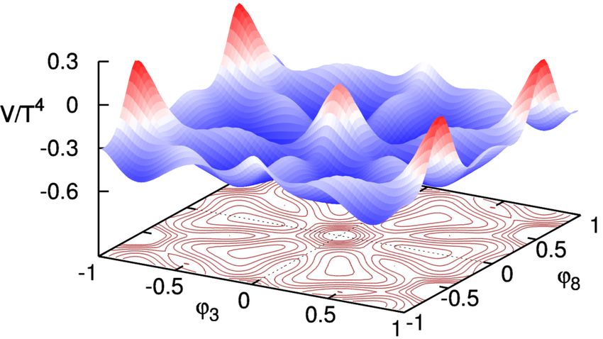
12μ
(a) Real chemical potential (chiral transition only). (b) Imaginary chemical potential.
A B C D
TRW TRW TRW TRW
Tc Tc Tc Tc
RW-transition RW-transition RW-transition RW-transition
1st order 1st order crossover 1st order
2nd order 1st order tricritical
2nd order
0 π/3 π 00 π/3 π 00 π/3 π 00 π/3 π
i µ/T i µ/T i µ/T i µ/T
(c) Left to right: phase diagrams in the temperature imaginary chemical potential plane at points A-D of Fig. 2.4b
(Nc = 3).
Figure 2.4: Extensions of Columbia plot to finite chemical potential and resulting phase diagrams.
be explored further.
The extension of the Columbia plot to imaginary chemical potential, at least for heavy quark masses, stands
on firmer ground. First, lattice calculations for imaginary chemical potential do not suffer from the sign prob-
lem. Second, effective theories for heavy quarks are available that can be simulated with low CPU costs
even at real chemical potential [144, 175]. Third, much can be learned from symmetry considerations alone.
Introducing the dimensionless variable θq ≡ Im(µq )/T with quark chemical potential µq and taking center
symmetry into account, Roberge and Weiss found that the physics of the theory is invariant under changes of
θ → θ + 2π/Nc with Nc the number of colours [176]. This symmetry is smoothly realised at low temperatures,
but occurs via a first order phase transition at large temperatures beyond TRW . The situation in the temperature
imaginary chemical potential plane is sketched in Fig. 2.4c. Above TRW the regions [0, π/Nc [, ]π/Nc , 3π/Nc [,
and ]3π/Nc , 5π/Nc [ are distinguished by the Polyakov loop L = |L|e−iφ , whose phase φ changes by 2π/Nc at
every first order RW-transition line. The point where the first order RW-transition lines end are touched by
the confinement/chiral transition lines with temperature. Depending on the values of the quark masses, i.e.
on the location in the Columbia plot, these transitions are of different order, as visualised in Fig. 2.4c for the
locations A (1st order region), B (second order critical line), C (slightly in the cross-over region) and D at
µ = 0 displayed in Fig. 2.4b. The point D is defined to be on the line in the mass plane where the second order
critical surface of the deconfinement transition intersects the plane with iµq /T = π/3. For points further out in
the crossover region the deconfinement transition is a crossover everywhere, regardless of the value of iµq /T .
It has been shown [144] that the tricritical point occurring at the intersection of the RW-transition with the
deconfinement transition for D strongly influences the whole second order critical surface in the sense that it
can be parametrised by tricritical scaling relations. We will came back to this issue in section 4.1, where we
discuss results from the DSE-framework for the critical surface.
The critical surfaces for the chiral transition, also sketched in Fig. 2.4b are much harder to evaluate on
the lattice, since the corresponding quark masses are small and therefore simulations very cost intensive.
Nevertheless it is very interesting to map these out, since this may give vital clues on the issue of the order of
the transition in the two-flavour theory, discussed above. The situation sketched in Fig. 2.4b corresponds to the
scenario with broken UA (1)-anomaly, i.e. the left plot of Fig. 2.3. If it were established that the critical surface
13intersects the left backplane of Fig. 2.4b above the µ = 0 plane for all quark masses, then the other scenario
of Fig. 2.3 is realised. Again, simulations have been performed indicating that this may very well be the case
[109, 164, 165], with the (important) caveat that a continuum extrapolation has not yet been done.
143 Non-perturbative quark and glue
In the previous section we discussed general aspects of the QCD phase diagram at finite temperature and
baryon chemical potential, highlighted the merits of theoretical studies at unphysical external parameters such
as quark masses or imaginary chemical potential and summarised briefly the connection to heavy ion collision
experiments via fluctuations of conserved charges. In this section we focus on the technical aspects of the
functional approach to QCD via Dyson-Schwinger equations (DSEs). We deal with the derivation of the DSEs,
explain the extraction of order parameters from the correlation functions of the theory and discuss strategies
for devising truncations that can be systematically tested and improved.
Readers interested in the available results at finite T and µ but not in the technical details of the framework
are encouraged to skip this section in a first reading and proceed to section 4. In order to appreciate the details
of the calculations and to understand the level of the rigorousness of the results, revisiting section 3 afterwards,
however, may be beneficial.
3.1 Functional equations
We work with the Euclidean version of the QCD generating functional that describes strongly interacting matter
in thermodynamical equilibrium as a grand-canonical ensemble. The gauge fixed partition function Z[T, µ] is
given by6 ˆ
Z[T, µ] = N D[AΨ̄Ψcc̄] exp − SQCD [A, Ψ, Ψ̄] − Sgf [A, c, c̄] , (3.1)
with the QCD gauge invariant action
ˆ ˆ
1/T X 1 a a
SQCD = − dx4 d3 x / + mq − µq γ4 ) Ψq + Fµν
Ψ̄q (−D Fµν , (3.2)
0 4
q=u,d,s,...
and the gauge fixing part
ˆ ˆ !
1/T
3 (∂µ Aµ )2
Sgf = dx4 d x − i∂µ c̄Dµ c . (3.3)
0 2ζ
Quarks with flavour q and bare masses mq are represented by the Dirac fields Ψq and Ψ̄q . Local gauge symmetry
of the quark fields demands the introduction of a vector field Aaµ , which represents gluons. The gluon field
a is given by
strength Fµν
a
Fµν = ∂µ Aaν − ∂ν Aaµ − gf abc Abµ Acν , (3.4)
with the coupling constant g and the structure constants f abc of the gauge group SU (Nc ), where Nc is the
number of colours. The covariant derivative in the fundamental representation of the gauge group is given by
Dµ = ∂µ + igAµ , (3.5)
with Aµ = Aaµ ta and the ta are the generators of the gauge group. We work with fixed gauge using the
Faddeev-Popov procedure [179] (see [180, 181] for pedagogical treatments of the subject) which introduces
the Grassmann valued Faddeev-Popov ghost fields c and c̄. The integral over the gauge group is absorbed in the
normalisation N . The gauge parameter is denoted by ζ. Below we always use Landau gauge, which is defined
by the gauge condition ∂µ Aµ = 0 and gauge parameter ζ = 0. 7
6
An introduction into path integral methods in quantum field theories is given e.g. in [177]. In the following we adhere to the
conventions of the review article [178].
7
Gauge fixing via the Faddeev-Popov procedure is well-known not to be complete and leaves one to deal with the problem of
Gribov-copies, i.e. multivalued instances of ∂µ Aµ = 0 for gauge field configurations related by gauge transformations (see the reviews
[182, 183] for a detailed account of the problem). This problem has been studied intensively on the lattice [184–188] and found to be
relevant for the behaviour of ghost and gluon propagators at very small momenta much below the temperature scales we are interested
in. Thus for the topic of this review we can safely ignore this problem.
15Renormalization of the QCD action entails the introduction of suitable counterterms. The correspondence
between the bare Lagrangian (3.2,3.3) and its renormalised version is given by the following rescaling trans-
formations
p
Aaµ → Z3 Aaµ , c̄a cb → Z̃3 c̄a cb , Ψ̄Ψ → Z2 Ψ̄Ψ, (3.6)
g → Zg g, ζ → Zζ ζ, (3.7)
where five independent renormalisation constants Z3 , Z̃3 , Z2 , Zg and Zζ have been introduced. Furthermore
five additional (vertex-) renormalisation constants are related to these via Slavnov–Taylor identities,
3/2 1/2 1/2
Z1 = Zg Z3 , Z̃1 = Zg Z̃3 Z3 , Z1F = Zg Z3 Z2 , Z4 = Zg2 Z32 , Z̃4 = Zg2 Z̃32 . (3.8)
In general, these renormalisation constants depend on the renormalisation scheme, the renormalisation scale µ
and the regularisation procedure. In the numerical treatment of Dyson-Schwinger equations, further detailed
below, it is common to use either a hard cut-off or a Pauli-Villars type regulator, resulting in a generic depen-
dence of the renormalisation constants on a regularisation scale Λ, i.e. Zi = Zi (µ, Λ). Provided multiplicative
renormalisability is not violated in the process of truncating the DSEs, all Green’s functions extracted from
the renormalised DSEs are independent of Λ and therefore do not suffer from divergences when Λ is sent to
infinity8 . This technical issue is well under control and further detailed in appendix A.
The generating functional (3.1) depends on temperature via the restriction of the x4 -integration from zero
to 1/T := β. In the imaginary time Matsubara formalism, which we adopt throughout this review, all fields
obey (anti-)periodic boundary conditions such that φ(x4 ) = ±φ(x4 +1/T ) for a generic field φ. Due to the Kubo-
Martin-Schwinger condition bosons (i.e. gluons) need to have periodic boundary conditions, while fermions
(quarks) have anti-periodic boundary conditions. The Faddeev-Popov ghosts are the exception from this rule
with periodic boundary conditions despite their Grassmann nature due to their origin from the gauge fixing
procedure [191]. In momentum space, this translates into momentum vectors p = (p, ωn ) with Matsubara
frequencies ωn = πT (2n + 1) for fields with antiperiodic boundary conditions and ωn = πT 2n for those with
periodic boundary conditions with integers n running from minus to plus infinity.
The quark chemical potential µq is added to the QCD action via a Lagrange multiplier −nq µq for the net
quark density
ˆ 1/T ˆ
nq = dx4 d3 x Ψ† Ψ (3.9)
0
with Ψ† = Ψ̄γ4 and is subsequently absorbed into the quark part of the QCD Lagrangian, cf. Eq (3.2). For
non-zero chemical potential the Matsubara frequencies for fermions are modified into ω̃n = ωn − iµ.
Starting from the generating functional (3.1) one can derive the Dyson-Schwinger equations for the Green’s
functions of the theory. In the following we outline the formalism in a very dense, symbolic notation. Readers
interested in more details are referred to the textbooks [177, 192] or the reviews [178, 193]. Dyson-Schwinger
equations follow from the generating functional (3.1) and the fact that the integral of a total derivative van-
ishes, i.e.
ˆ ( ˆ 1/T ˆ )
δ 3
0 = D[AΨ̄Ψcc̄] exp −SQCD − Sgf + dx4 d x AJ + η̄Ψ + Ψ̄η + σ̄c + c̄σ
δφ 0
δ(SQCD + Sgf )
= − +j (3.10)
δφ
for any field φ ∈ {A, Ψ, Ψ̄, c, c̄} and its corresponding source j ∈ {J, η, η̄, σ̄, σ}. Equation (3.10) is correct pro-
vided that the functional integral (3.1) is well-defined and the measure D[AΨ̄Ψcc̄] is translational invariant.
Acting onto (3.10) with a suitable number of further functional derivatives and setting all sources to zero after-
wards leads to the Dyson-Schwinger equation (DSE) for any desired full n-point function. A similar procedure
8
Within quenched QED, the independence of the resulting Green’s functions from the employed regularisation scheme has been
studied and shown to hold in Ref.[189, 190]
16applied to the generating functional W = ln(Z) or the effective action Γ = W + hφij leads to the DSEs for
connected Green’s functions and the ones for one-particle irreducible Green’s functions. The expression (3.1)
and its functional derivatives constitute an infinite tower of coupled integral equations. Provided QCD is a local
quantum field theory, this infinite tower contains all physics of the original path integral, cf. the review article
Ref. [178]. Below we will analyse some of these equations in more detail.
Closely related to the formalism of Dyson-Schwinger equations is the one for the functional renormalization
group (FRG), see [194, 195] and the reviews [196–199]. The basic idea of this approach is to endow the gen-
erating functional with an (infrared) cut-off scale k which suppresses all quantum fluctuations with momenta
<
q 2 ∼ k 2 smaller than this scale. The resulting effective action Γk depends on the cut-off scale and satisfies a
functional differential equation which controls this dependence. Lowering k takes into account more and more
quantum fluctuations characteristic for the scale k in question. In this way one can explore the relevant physics
in a systematic way. Finally, sending k → 0 recovers the full effective action of the theory. By taking functional
derivatives of the functional differential equation one obtains an infinite tower of coupled integro-differential
equations for the Green’s functions of the theory, which are not too dissimilar in structure to the tower of
Dyson-Schwinger equations. Thus, in principle it is possible to explore the physics content of the Green’s func-
tions of QCD from both frameworks, the DSE and the FRG tower of equations. Interestingly, the combination
of both methods sometimes leads to unique results, see [200, 201] for an example. In this review article we
focus primarily on results for QCD at finite temperature and density obtained in the DSE approach, but we
make connections to corresponding or complementary results from the FRG-framework wherever possible.
A third functional framework that has been employed for QCD at finite temperature and chemical potential
is the variational Hamilton approach in various formulations [202–208]. For all technical details we refer the
interested reader to the original literature and the review article Ref. [209]. Similar to other functional methods
one ends up with a coupled set of integral equations for the Green’s functions of the theory which have to be
solved using numerical methods. Again, in the following we do not review the corresponding results in any
detail but make connections to the DSE results discussed in this review wherever appropriate.
Finally, there is growing interest in a fourth framework based on functional methods, the Gribov-Zwanziger
approach. This approach is based on studies of the effects of gauge fixing on the theory and the desire to
eliminate the effects of Gribov copies [210, 211]. As a result one arrives at an effective action which contains a
new scale, the Gribov parameter, which affects the gluon dispersion relation and changes its infrared behaviour,
see [183] for a review on the technical details. This approach was generalized to finite temperature in [212].
Somewhat related to the Gribov-Zwanziger approach is the one of [213, 214] based on the Curci-Ferrari model.
Both, the Gribov-Zwanziger framework and the Curci-Ferrari model have been used at finite temperature and
chemical potential, and heavy quark physics and transport properties of the quark-gluon plasma have been
explored [148, 149, 215–219]. Again, we will not discuss these results in detail but point the interested reader
to the literature wherever appropriate.
3.2 Quarks, gluons and order parameters
The DSEs for the ghost, gluon and quark propagators are given diagrammatically in figure 3.1. They form
a coupled system of equations which demand dressed ghost-gluon, three-gluon, four-gluon and quark-gluon
vertices as input.9 These three- and four-point functions satisfy their own DSEs, which in turn contain four-
and five-point functions and so on. In order to solve the tower of DSEs one has to choose a truncation scheme,
i.e. a strategy to break down the infinite tower into a closed system of equations. We will come back to ponder
on strategies to make this procedure systematic in subsection 3.3 below. Here we wish to focus first on the
relation of the propagators of QCD to suitable order parameters for the phase transitions at finite temperature
9
The corresponding equations in the framework of the functional renormalization group display a number of interesting structural
differences. First, they do not feature two-loop diagrams, as are present in the DSE for the gluon propagator. From the point of view of
the practitioner aiming at numerical solutions for these equations, this is clearly an advantage. On the other hand, however, the FRG
equations contain more unknown four-point functions (such as a fully dressed ghost-gluon scattering kernel and others), which need
to be specified in order to close the equations. Also, besides being integral equations, the FRGs contain derivatives with respect to the
FRG-scale k. Thus, both formulations of functional equations present their own challenges which more or less balance out and it is
often only a matter of personal taste and experience which ones to choose.
17You can also read