Heavy-flavor hadro-production with heavy-quark masses renormalized in the MS, MSR and on-shell schemes
←
→
Page content transcription
If your browser does not render page correctly, please read the page content below
Published for SISSA by      Springer
                                                                      Received: October 8,   2020
                                                                      Revised: January 27,   2021
                                                                    Accepted: February 22,   2021
                                                                       Published: April 6,   2021

Heavy-flavor hadro-production with heavy-quark

                                                                                                    JHEP04(2021)043
masses renormalized in the MS, MSR and on-shell
schemes

M.V. Garzelli,a L. Kemmler,a S. Mocha,b and O. Zenaievc
a
  II. Institute for Theoretical Physics, Hamburg University,
  Luruper Chaussee 149, D-22761 Hamburg, Germany
b
  MTA-DE Particle Physics Research Group,
  PO Box 105, HU-4010 Debrecen, Hungary
c
  CERN,
  CH-1211, Geneva 23, Switzerland
    E-mail: maria.vittoria.garzelli@desy.de,
    lkemmler@physnet.uni-hamburg.de, sven-olaf.moch@desy.de,
    oleksandr.zenaiev@cern.ch

Abstract: We present predictions for heavy-quark production at the Large Hadron Col-
lider making use of the MS and MSR renormalization schemes for the heavy-quark mass
as alternatives to the widely used on-shell renormalization scheme. We compute single and
double differential distributions including QCD corrections at next-to-leading order and
investigate the renormalization and factorization scale dependence as well as the perturba-
tive convergence in these mass renormalization schemes. The implementation is based on
publicly available programs, MCFM and xFitter, extending their capabilities. Our results
are applied to extract the top-quark mass using measurements of the total and differential
tt̄ production cross-sections and to investigate constraints on parton distribution functions,
especially on the gluon distribution at low x values, from available LHC data on heavy-
flavor hadro-production.

Keywords: NLO Computations, QCD Phenomenology

ArXiv ePrint: 2009.07763

Open Access, c The Authors.
                                                        https://doi.org/10.1007/JHEP04(2021)043
Article funded by SCOAP3 .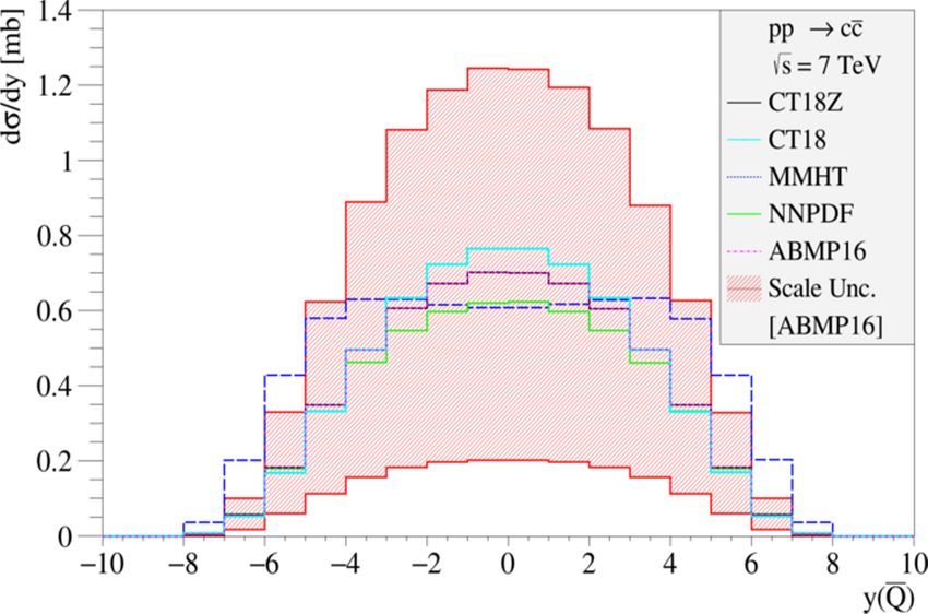
Contents

1 Introduction                                                                               1

2 Implementation of heavy-quark mass renormalization schemes                                 3

3 Predictions for differential cross-sections                                                8

4 Phenomenological applications                                                             31

                                                                                                  JHEP04(2021)043
  4.1 Extraction of mt (mt ) and mMSR
                                  t    + αS (MZ ) from differential tt̄
      cross-sections at NLO                                                                 31
  4.2 NLO PDF fits with differential charm hadro-production cross-sections                  35
  4.3 NNLO PDF fits with total charm hadro-production cross-section                         36

5 Conclusions                                                                               42

1   Introduction

Charm-anticharm and bottom-antibottom pair-production are among the most frequent
inelastic processes occurring in hadronic collisions at the Large Hadron Collider (LHC),
with cross-sections smaller than for the dijet case but well above those for the top-antitop
case, as follows from the hierarchy of the heavy-quark masses, the available phase-space,
and the structure of the Standard Model (SM) Lagrangian.
     Heavy quarks are not observable as free asymptotic states. Charm- and bottom-quarks
hadronize, due to confinement, whereas the top-quark decays before hadronizing, due to
its large decay width. Collider experiments implement procedures for reconstructing top-
quarks from their decay products and are able to detect the products of the hadronization
/ fragmentation of intermediate-mass quarks, i.e. heavy mesons and baryons, as well as the
jets associated to them, i.e. b-jets and c-jets. B-hadrons and D-hadrons are reconstructed
by their decay products, with decay vertices displaced with respect to the primary vertex.
This operation requires good tracking, vertexing and particle identification capabilities.
The measurements are indeed easier to perform in case of B-hadrons than for D-hadrons,
because the proper lifetimes of the first ones are longer than those of the latter.
     On the theory side, analytical formulae for the hadro-production of massive quark pairs
are known since many years in quantum chromodynamics (QCD) perturbation theory at
the next-to-leading order (NLO) accuracy, both for the total cross-sections as well as for
one-particle inclusive differential distributions [1–5]. More recently, next-to-next-to-leading
order (NNLO) QCD predictions have been computed for the total cross-sections of heavy-
quark pair-production [6–9]. On the other hand, differential predictions at NNLO are
available for top-quark pair production [10, 11], but not yet for the case of charm-quark

                                            –1–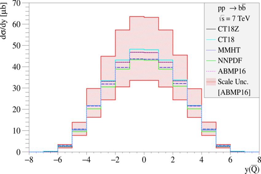
pair. Very recently, a first computation of differential cross-sections for bottom-quark pair
production including NNLO QCD corrections has appeared [12].
      Beyond fixed-order perturbation theory, the resummation of logarithms in the ratio
pT /m, relevant when the transverse momentum of the heavy-quark pT is much larger than
its mass m, up to the next-to-leading-logarithmic accuracy, performed through the frag-
mentation function approach [13], has been combined with NLO predictions [14–16]. The
resummation of recoil logarithms related to soft gluon radiation from initial state partons,
as well as the one of threshold logarithms and high-energy logarithms, have also been
worked out (up to various degrees of accuracy) and presented in a number of papers (see
e.g. [17–22]). The transition from quarks to hadrons is described either by fragmenta-

                                                                                                  JHEP04(2021)043
tion functions (FFs) [23–25], or by matching NLO matrix elements to parton shower and
hadronization approaches [26–30].
      One of the inputs of all aforementioned calculations are the values of the heavy-quark
masses. The SM by itself does not predict the values of the quark masses, which are thus
fundamental parameters and subject to renormalization. The ultraviolet divergences ap-
pearing in the heavy-quark self-energies, to be eliminated by renormalization, require to
fix a specific renormalization scheme for relating the bare masses to the renormalized ones.
The most common choice is the mass in the on-shell scheme, defining the pole mass by
the relation that the inverse heavy-quark propagator with momentum p vanishes on-shell,
i.e. for p2 = (mpole )2 , and it is known at four loops in QCD [31, 32]. Another option, also
known at four loops [33, 34], is the MS prescription. In complete analogy to the renormal-
ization of the strong coupling constant αS , only divergent terms are absorbed such that the
quark propagator becomes finite after wave-function and mass renormalization. Finally, the
MSR scheme [35] defines a scale-dependent short-distance mass, that interpolates smoothly
between a valid mass definition at low scales much below the mass and the MS mass for
scales larger than the mass, using infrared renormalization group flow. Thus, predictions
for physical observables in perturbation theory carry scheme dependence through the choice
of a particular mass renormalization scheme. For a given observable, the behavior of the
truncated expansion in perturbative QCD, including the apparent convergence and the
residual scale dependence, can vary significantly between different schemes employed.
      In this paper we describe the phenomenological effects of the use of the MS and MSR
schemes for the renormalization of the heavy-quark masses in charm, bottom and top pro-
duction at hadron colliders. We investigate the perturbative convergence in these schemes,
by providing comparisons between physical quantities calculated at various levels of ac-
curacy, and we discuss applications concerning the extraction of mass values and parton
distribution functions (PDFs) from collider data.
      Various phenomenological and experimental investigations on top quark hadro-pro-
duction with top mass renormalized in the MS scheme already exist in the literature (see
e.g. [36–42]). On the other hand, the MSR mass is discussed in various theory papers,
mainly focusing on its definition and properties (see e.g. [43–45]). As for the top quark case,
the main novelties of our work are the phenomenological predictions for NLO differential
cross-sections in pp collisions using the MSR mass, which we compare to those with the MS
and pole masses in a consistent framework, the implementation of a dynamical mass renor-

                                            –2–
malization scale in the computation of transverse momentum distributions of the heavy-
quarks, as an alternative to the static m(m) case, and the extraction of a top MSR mass
value from the analysis of state-of-the-art LHC triple-differential cross-section data, previ-
ously used for extracting m(m) [46]. The extraction is done preserving correlations with the
strong coupling constant αS and the PDFs, fitted simultaneously to the heavy-quark mass.
     Total cross-sections for charm and bottom production at hadron colliders with the mass
renormalized in the MS scheme are available since a while [47]. The MS scheme has also
been used for heavy-quark production in deep-inelastic scattering (DIS), which has allowed
extractions of the charm mass mc (mc ) and bottom mass mb (mb ) (see e.g. [48–50]). On the
other hand, differential cross-sections for charm and bottom production at hadron colliders

                                                                                                 JHEP04(2021)043
with MS and MSR masses have never been presented in a dedicated phenomenological
paper before this one, to the best of our knowledge. We show examples of them here for
the first time and discuss the relative uncertainties due to scale and mass variation, working
at NLO accuracy. In case of MS cross-sections we also show the role of variations of the
heavy-quark mass renormalization scales, comparing their effects to those induced by the
variation of other scales appearing in fixed-order computations, i.e. the factorization and
αS renormalization scales.
     In recent years heavy-flavor hadro-production data at the LHC have been used to con-
strain gluon and sea quark distributions at small x in PDF fits at NLO, working in the
on-shell mass renormalization scheme [51–54]. In this work we comment on the simulta-
neous extraction of proton PDFs and the charm mass in the MS scheme, as an alternative
to the pole scheme, using LHCb and HERA data and a fitting procedure were everything
else is the same, except the charm mass renormalization scheme. Our findings at NLO
support the use of masses renormalized in the MS scheme for further fits of this kind (see
e.g. [55, 56]). We also show for the first time how LHC charm production data extrapolated
to the full phase-space can be used to constrain NNLO PDF fits, suggesting a reduction of
the uncertainties in the gluon distributions of various widely used global PDF fits [57–59].
     The implementation of the MS and MSR schemes for renormalizing the heavy quark
masses, as an alternative to the on-shell scheme, is described in section 2. The obtained
theoretical predictions for differential distributions including NLO QCD corrections and
mass renormalization in these three schemes, are presented in section 3, together with
considerations on the convergence of the perturbative expansion in the strong coupling
constant. The results are applied in section 4 to investigate the impact of LHC data
on possible extractions of PDFs from collider data and on determinations of the heavy-
quark mass values in different mass renormalization schemes. In section 4.3, we also use
predictions for total cross-sections of charm hadro-production up to NNLO accuracy in
QCD. Finally, our conclusions are summarized in section 5.

2   Implementation of heavy-quark mass renormalization schemes

In this work light quarks are assumed to be massless. For the heavy-quark masses, on
the other hand, different renormalization schemes can be adopted and we briefly recall
the relevant relations for the above mentioned cases of the MS, MSR and on-shell schemes.

                                            –3–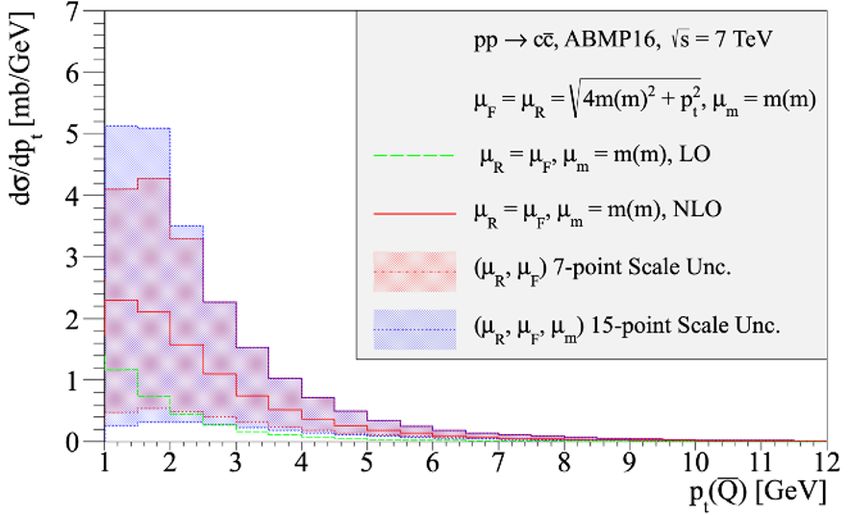
Other choices for the mass renormalization are possible. For physical observables inherently
connected to the heavy-quark production threshold, for instance, the potential subtracted
mass [60] was suggested as a possibility to produce an improved perturbative convergence at
energies slightly above the quark-pair production threshold and the 1S mass has been pre-
sented [61] as a way of stabilizing the position of the peak of the vector-current-induced total
cross-section for tt̄ production in e+ e− collisions, as a function of the center-of-mass energy
√        √
   s, for s ∼ 2m. In boosted kinematics, limited to the case of top-quarks, the top-quark
jet-mass [62], was introduced in the framework of Soft Collinear Effective Theory. Further
mass renormalization schemes are described, e.g., in refs. [44, 45] and references therein.
      The on-shell mass coincides with the pole in the propagator of the renormalized quark

                                                                                                    JHEP04(2021)043
field and is known up to four loops in QCD [31, 32]. Thus, it is the same at all scales and
infrared finite to all orders in perturbation theory. This definition of the pole mass mpole ,
although being gauge invariant, has its short-comings [63, 64]. It does not extend beyond
perturbation theory, i.e. to full QCD, since it is based on the (unphysical) concept of colored
quarks as asymptotic states. Therefore, mpole must acquire non-perturbative corrections,
which leads to an intrinsic uncertainty in its definition of the order O(ΛQCD ) related to
the renormalon ambiguity [65]. The latter manifests itself as a linear sensitivity to infrared
momenta in Feynman diagrams, leading to poorly convergent perturbative series for the
observables expressed in terms of mpole .
      On the other hand, short-distance mass definitions such as the MS or the MSR schemes
are renormalon-free. In general, such short-distance masses msd are related to the pole mass
through the relation
                            mpole = msd (R, µR ) + δmpole-sd (R, µR ) ,                     (2.1)
where the term δmpole-sd removes the renormalon and the dependence of the short-mass
definition on long-distance aspects of QCD. Here, µR denotes renormalization scale, con-
nected with the ultraviolet divergences, whereas the scale R is associated with the infrared
renormalization group equation (RGE) [35]. In many short-distance mass renormalization
schemes, R coincides with the renormalized mass itself, as for instance in the MS scheme,
where R = m(µR ). However, the possibility to consider other choices of R through the
associated RGE allows to improve the stability of the conversion between short-distance
mass schemes characterized by different values of R.
     In the MS scheme, the renormalized mass of the heavy quark evolves with the RGE in
the renormalization scale µR , governed by the mass anomalous dimensions γ(αS (µR )),
                                   dm(µR )
                             µ2R           = −γ(αS (µR )) m(µR ) ,                         (2.2)
                                    dµ2R

where the perturbative expansion of γ(αS (µR )) ≡ ∞                         i+1 is known at four
                                                      P
                                                        i=0 γi (αS (µR )/π)
loops [33]. Precise determinations of the MS masses for charm- and bottom-quarks are
summarized by the Particle Data Group (PDG) [23]. For the MS mass of the top-quark,
see, e.g., refs. [23, 40, 41, 49, 66]. The conversion to the on-shell scheme proceeds in the
standard manner
                                                   ∞           !
                                                           αS i
                                                  X
                                pole
                              m      = m(µR ) 1 +     ci            ,                      (2.3)
                                                  i=1
                                                            π

                                              –4–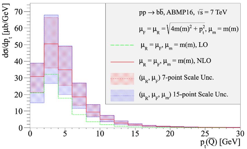
where the first numerical coefficients ci read [67–69],

                    4
               c1 =    + L,                                                                                       (2.4)
                    3
                    307           2       1     509    47
               c2 =       + 2ζ2 + ζ2 ln2 − ζ3 +     L + L2
                     32          3       6     72     24
                         71     1     13    1 2        4 X          mi

                    −        + ζ2 + L + L nlf +                ∆            .                                     (2.5)
                         144 3        36    12         3 1≤i≤n     m(µR )
                                                                             lf

Here, ζ denotes the Riemann zeta-function, L ≡ ln(µ2R /m(µR )2 ) and the function ∆ ac-
counts for all quarks with masses mi smaller than the heavy-quark one. As the light quarks

                                                                                                                          JHEP04(2021)043
are taken massless here, i.e., mi = 0, the ∆ term vanishes. The strong coupling αS is eval-
uated at the scale µR and renormalized in the MS scheme with the number of active flavors
set to nf = nlf + 1 at and above the heavy-quark threshold scale, which is assumed to be
equal to its running mass. The number of light flavors is nlf = 3, 4, 5 for charm, bottom
and top production, respectively.
     For the particular choice m(m) ≡ m(µR = m(µR )), i.e. the MS mass renormalized
at the specific scale µR = m(µR ), the logarithmic terms L cancel and eq. (2.3) evaluates
numerically (up to terms O(αS4 )) as [70]
                            "                                                              2
                                             αS                                       αS

             pole
           m        = m(m) 1 + 1.333                  + (13.44 − 1.041 nlf )
                                             π                                        π
                                                                                                          #
                                                                             α 3
                                                                                  S
                                + 190.595 − 27.0 nlf +         0.653 n2lf                  +    O(αS4 )       .   (2.6)
                                                                                  π

The infrared renormalon ambiguity in the conversion in eqs. (2.3), (2.6) manifests itself in
practice as factorially growing terms in the perturbative expansion, that spoil convergence.
The sizable coefficients in eq. (2.6) indicate the poor convergence of mpole for the case
of charm and bottom, when αS at low scales is large. For top-quarks, the convergence
is better due to the smaller value of αS at larger scales. Including the four-loop QCD
results [33, 34], the residual uncertainty in mpole for top-quarks, including renormalon
contributions, is estimated of the order of a few hundred MeV [71], i.e., of the order of
O(ΛQCD ). All available relations for scheme changes from m(µR ) to mpole and vice versa
have been summarized in the programs CRunDec [72] and RunDec [73].
     While αS in eqs. (2.3), (2.6) is renormalized in the MS scheme, the matrix elements,
as well as the PDFs and the associated αS evolution used in the fixed-order massive calcu-
lations presented in this paper are all defined with a fixed number of light flavors nlf = 3
for charm and bottom production1 and nlf = 5 for top production, even at scales well
above the heavy-quark mass value. For αS renormalization in the decoupling scheme [77],
subtractions in graphs with light-quark loops are done at zero mass, as in the MS scheme,
whereas those in graphs with heavy-quark loops are done at zero momentum. The heavy
quarks therefore do not contribute as active flavors to the running of αS in the effective
   1
    The use of nlf = 3 even for bottom production is justified for bottom-quark production at very low pT
(see e.g. the available measurements of B-meson production by the LHCb collaboration [74–76]).

                                                      –5–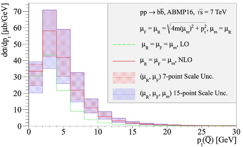
theory. Factorization is performed in the same scheme, which implies the use of non-
vanishing PDFs only for light partons, and a calculation of partonic cross-sections done
consistently. The latter is achieved by including contributions of virtual amplitudes cor-
responding to Feynman diagrams with massive heavy-quark fermionic loops. For the case
of bottom production in the 3-flavor scheme, we verify that including or not the relevant
charm-loop diagrams in our computations, assuming mc = 0, produces differences well
within 1% on the total cross-section of bb̄ hadro-production. We argue that including a
charm mass different from zero, as appropriate for a fully consistent calculation in the
3-flavor scheme, makes also a small effect, well below the uncertainties on cross-sections
due to scale variations. This effect compensates only partially the differences due to the

                                                                                                 JHEP04(2021)043
modified αs value, that, at renormalization scales of the order of the bottom quark mass,
is a few percent lower in the scheme with nf = 3 active flavors, with respect to the nf = 4
case. Possible advantages of computing bottom production in the 3-flavor scheme have also
been claimed in the framework of DIS calculations [78, 79], where the effects of including a
finite charm-mass in the fermionic loop corrections turn also out to be small. We observe
that our predictions for bottom production typically differ by some percent from those of
fully consistent calculations with matrix-elements, PDFs and αS in the 4-flavor scheme,
depending on the input.
     Using the standard decoupling relations, it is possible to relate the PDFs, αS and the
partonic cross-sections in the MS and decoupling schemes, once the matching scale is fixed.
In this way, also eqs. (2.3), (2.6) can be re-expressed in terms of αS with the heavy degrees
of freedom decoupled. If the decoupling is performed at a scale equal to the MS mass
m(m), the coefficients c1 and c2 in eqs. (2.4), (2.5) remain identical due to the fact that
                                                               (n +1)       (n )
the leading order coefficient in the decoupling relation for αS lf     to αS lf vanishes.
     In practice, although the perturbative expansion in eqs. (2.3), (2.6) is known up to four
loops [33], we truncate it in this work to two loops (order αS2 ) for computing the NNLO
cross-sections and to one loop (order αS ) for computing NLO cross-sections, respectively,
unless stated otherwise. In addition, the evolution of αS as a function of µR and the
corresponding αS values entering in eqs. (2.3), (2.6) and other parts of the fixed-order
computation are evaluated retaining three loops for producing NNLO cross-sections and
two loops for producing the NLO ones, respectively, unless stated otherwise.
     The MSR mass is a specific realization of the short-distance mass introduced in
eq. (2.1). It is obtained, e.g., by considering the difference between mpole and m(m),
see eq. (2.3), and substituting m(µR ) with R in the terms proportional to αS to determine
the difference between mpole and mMSR (R) as
                                                  ∞                       i
                                                                 αs (R)
                                                  X
                         mpole = mMSR (R) + R           ai                     ,         (2.7)
                                                  i=1
                                                                   π

where the numerical coefficients ai are given in ref. [35]. The evolution of the MSR mass
with the R scale follows the RGE

                                dmMSR (R)
                            R             = −R γ MSR (αS (R)) ,                          (2.8)
                                  dR

                                            –6–
3                                                            3
m(µ) [GeV]   10                                                        10

                                                           mMSR(R) [GeV]
                                           mc(µ)                                                             mMSR
                                                                                                              c  (R)
                                           mb(µ)                                                             mMSR
                                                                                                              b  (R)
                                           mt (µ)                                                            mMSR
                                                                                                              t  (R)

             102                                                       102

             10                                                            10

                  1                                                         1

                                                                                                                           JHEP04(2021)043
       10−1                                         3
                                                                    10−1                                               3
                   1   10            102           10                           1        10            102          10
                                              µ [GeV]                                                          R [GeV]

Figure 1. The one-loop evolution of the MS charm-, bottom- and top-masses for varying renor-
malization scales µ (left). The one-loop evolution of the MSR charm-, bottom- and top-masses for
varying scales R (right). The values of µ and R used in the subsequent calculations and figures of
this work are marked with filled dots. The value of αS (MZ ) is fixed to 0.118 and αS is evolved at
four loops, as in table 1.

which is linear in the scale R and where γ MSR (αS (R)) ≡ ∞    MSR (α (R)/π)i+1 denotes
                                                                                    P
                                                          i=0 γi     S
the R scheme anomalous dimension. In practice, the MSR mass interpolates between the
pole and the MS mass m(m). This occurs through the dependence on the scale R, because
by construction mMSR (R) → mpole for R → 0 and mMSR (R) → m(m) for R → m(m).
     In the following we use what has been called practical MSR mass in ref. [43], in con-
trast to the natural MSR mass. For our purposes the numerical differences between those
definitions are mostly negligible.
     The evolution of the MS heavy-quark masses with renormalization scale is shown in
the left panel of figure 1. It is calculated at one loop using the CRunDec program [72, 73]
(nlf = 3 for charm and bottom, nlf = 5 for top). The evolution of the MSR heavy-quark
masses with the R scale at one loop is shown in the right panel of figure 1. It is obtained
by solving the RGE in eq. (2.8):

                                                        Z ln R
                            mMSR (R) = mMSR (R0 ) −                        R γ MSR (αs (R)) d ln R ,            (2.9)
                                                         ln R0

where expressions for the first few coefficients of the anomalous dimension γ M SR can be
found in refs. [35, 43]. Here, eq. (2.9) is expanded up to the lowest non-vanishing order
of αs . As is visible in figure 1, the MS mass values are decreasing with increasing values
of the renormalization scale µR . The MSR mass values are decreasing at increasing R
values, as follows from the form of the RGE for the R evolution and the fact that the
first coefficient γ0MSR in the perturbative expansion of the anomalous dimension γ MSR is
positive, cf. eq. (2.8).

                                                    –7–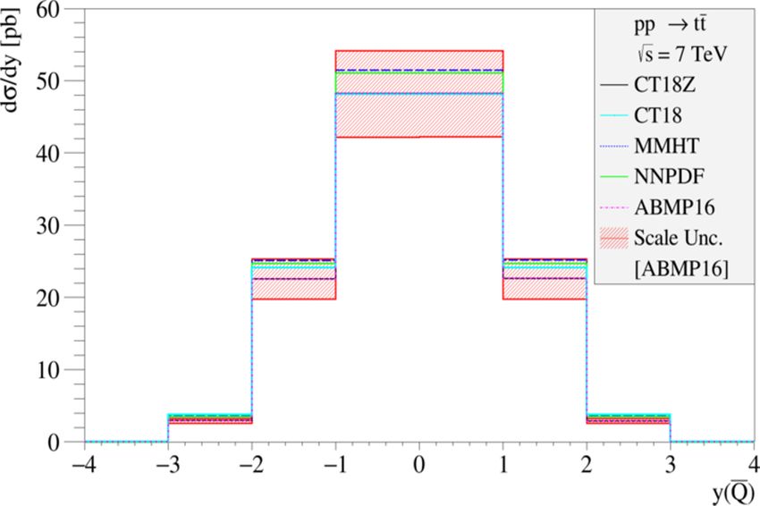
mMSR (1)       mMSR (3) mMSR (9)          m(m)    mpl
                                                        1lp   mpl
                                                                2lp mpl3lp         mpl
                                                                                    1lp   mpl
                                                                                            2lp mpl
                                                                                                  3lp
                  from m(m)                                from m(m)                  from MSR(3)
                                                 top-quark
        171.8        171.5        170.9       162.0 169.5 171.1 171.6              171.8       172.0   172.1
        172.9        172.5        171.9       163.0 170.5 172.1 172.6              172.9       173.0   173.1
        173.9        173.6        173.0       164.0 171.5 173.2 173.6              173.9       174.1   174.2
                                               bottom-quark
        4.69          4.30         3.67       4.15    4.53    4.74   4.90          4.61        4.80    4.97
        4.72          4.33         3.70       4.18    4.57    4.77   4.94          4.64        4.84    5.01

                                                                                                               JHEP04(2021)043
        4.75          4.36         3.74       4.21    4.60    4.81   4.97          4.68        4.87    5.04
                                                charm-quark
        1.33          0.94         0.31       1.25    1.46    1.68   1.98          1.25        1.44    1.61
        1.37          0.97         0.35       1.28    1.50    1.70   2.00          1.29        1.48    1.65
        1.40          1.01         0.38       1.31    1.53    1.73   2.02          1.33        1.52    1.69

Table 1. Numerical values for heavy-quark MSR, MS and pole masses. Columns 1–3 and 4 show
the MSR masses at different R scales (1, 3 and 9 GeV) and the MS mass from which they are
obtained [23, 66] using eq. (2.9) with the anomalous dimensions at three-loop for the R-evolution
of the MSR mass from the scale R0 = m(m) to R. Columns 5–7 show the one-, two- and three-loop
pole masses obtained from the conversion of the MS mass in eq. (2.3). Columns 8–10 show the
one-, two- and three-loop pole masses obtained from the conversion of the MSR mass at R = 3 GeV
using eq. (2.7). All values are given in GeV. In the conversion formulas between the expression of
masses in different renormalization schemes, we use the coupling constant αS of the effective theory
including 5 active flavors in case of top and 3 active flavors in case of charm and bottom, obtained
through decoupling from the theory including one additional quark, supposed to be massive. We
fix αs (MZ )nf =5 = 0.118 (αs (MZ )nf =3 = 0.106) and we evolve αS at four loops in all cases.

     In table 1 we compare the MS masses at the reference scale µref ≡ m(µref ), i.e. m(m),
for charm-, bottom- and top-quarks2 with the pole masses mpole , obtained from the previous
ones by retaining different numbers of terms in the conversion formula eq. (2.3), and the
MSR masses mMSR (R) at various numerical values of the R scale obtained by using eq. (2.9)
for the evolution. For top-quarks, the MSR mass value at R = 3 GeV is numerically close
to the values obtained in the on-shell scheme at two- or three loops. For bottom- or charm-
quarks on the other hand, the conversion of m(m) or mMSR (R) to the on-shell scheme
demonstrates the poor convergence of the perturbative expansion already discussed above,
cf. eq. (2.6).

3       Predictions for differential cross-sections

Predictions for cross-sections of heavy-quark production with different mass renormaliza-
tion schemes can be obtained from those in the widely used on-shell scheme by substituting
eqs. (2.3) and (2.7) in the cross-sections and performing a subsequent perturbative expan-
    2
        For the top-quark masses, such comparisons have already been presented in ref. [39].

                                                     –8–
sion in αs , see refs. [36, 38]. In particular, the cross-sections converted to the MS or MSR
mass schemes are determined to NLO accuracy as follows
                                                                                                   !
           MS                    pole    pole                                      pole     dσ 0
       σ        (m(µR )) = σ            (m      )                   +(m(µR )−m            )                       ,    (3.1)
                                                    mpole =m(µR )                           dm         m=m(µR )
                                                                                                           !
     MSR        MSR              pole    pole                               MSR            pole     dσ 0
 σ         (m         (R)) = σ          (m      )                     +(m         (R)−m           )                         .
                                                    mpole =mMSR (R)                                 dm         m=mMSR (R)

Here σ 0 is the Born contribution to the cross-section (proportional to O(αs2 )), and the
differences m(µR ) − mpole and mMSR (R) − mpole are calculated up to the lowest non-

                                                                                                                                JHEP04(2021)043
vanishing order in αs , such that all terms of order O(αs4 ) are dropped in eq. (3.1), as
appropriate for a NLO calculation at order O(αs3 ). Formulae for scheme conversions up to
NNLO haven been given in refs. [36, 38].
     We are considering theory predictions for stable heavy quarks (in case of bottom and
charm augmented by FFs to describe the final state B- and D-hadrons, as for the appli-
cations in section 4). The additional impact of parton showers and the dependence of the
quark mass parameter on their cutoff [80] as well as the study of renormalon effects in obser-
vables with cuts leading to corrections of order ΛQCD in the extracted quark masses [81]
are subject of ongoing theory research.
     We have computed double-differential cross-sections as functions of the transverse mo-
mentum pT and rapidity y of the heavy quark Q, and single-differential cross-sections as a
function of the invariant mass MQQ̄ of the heavy-quark pair in the on-shell, MS and MSR
mass renormalization schemes at NLO using both frameworks, MCFM [82, 83] with modifi-
cations [38, 84] and xFitter [85]. In both cases, the original NLO calculations are done in
the pole mass scheme [3, 4, 86]. The modified MCFM program [38] is capable of converting
the NLO calculations using a pole mass into those with the heavy-quark mass renormal-
ized in the MS mass scheme, in case of single-differential distributions in pT of the heavy
quark, y of the heavy quark and invariant mass MQQ̄ of the heavy-quark pair. On the
other hand, the developed xFitter framework implements the calculation of one-particle
inclusive cross-sections (i.e., with the other particle integrated over), i.e., it is capable to
compute the double-differential cross-sections as a function of pT and y of the heavy quark,
but not as a function of the invariant mass MQQ̄ of the heavy-quark pair. It converts the
pole-mass NLO cross-sections into the MS and MSR mass schemes for fully differential
distributions. The derivative of the Born contribution appearing in eq. (3.1) is calculated
semi-analytically in MCFM (see [38]), whereas it is computed numerically in xFitter, which
allows for cross-checks of both methods. The differential cross-sections in different schemes
which can be computed by MCFM and xFitter are summarized in table 2. For all cross-
sections calculated with both programs, MCFM and xFitter, (i.e. all those in the pole mass
scheme and the pT and y differential distributions in the MS mass scheme), agreement
within one percent accuracy is found.3 xFitter is also interfaced to other codes, like e.g.
   3
    The MCFM and xFitter differential cross-sections for the production of all heavy-quarks (the latter are
based on the program HVQMNR [86]) calculated using µR = µF agree within about 1%. In view of the large
scale uncertainties at NLO this level of agreement is satisfactory.

                                                              –9–
Cross-section pole mass scheme MS mass scheme MSR mass scheme
dσ/dpT M, X M, X X
dσ/dy M, X M, X X
dσ/dM M, X M –
d2 σ/dpT dy M, X X X
Table 2. Summary of the capabilities of the MCFM (M) and xFitter (X) frameworks to compute
differential cross-sections for heavy-quark hadro-production in different mass schemes.
JHEP04(2021)043
aMC@NLO, and thus it can be used for computing cross-sections with heavy-quark masses
renormalized in the MS scheme (instead of the pole scheme implemented in the standalone
standard version of these codes) for a wider range of processes (e.g. tt̄+j hadro-production,
see section 4.1 for the application of this interface to a phenomenological study).
In the calculations of the differential distributions presented in the following, we use
the PDG values [23] for the MS charm- and bottom-quark masses, mc (mc ) = 1.28 GeV and
mb (mb ) = 4.18 GeV, and the MS top-quark mass value mt (mt ) = 163 GeV [41]. Alterna-
tively, we use the MS charm-, bottom- and top-quark mass central values extracted from
the ABMP16 NLO simultaneous fit of PDFs, αS (MZ ) and MS heavy-quark masses [56]:
mc (mc ) = 1.18 GeV, mb (mb ) = 3.88 GeV and mt (mt ) = 162.1 GeV. Although these values
are smaller than those quoted by the PDG, they allow for fully self-consistent computa-
tions when used in association with the ABMP16 αS values and PDFs.4 The pole and
MSR mass values are obtained from the previous ones, using a procedure analogous to
that adopted for building table 1, except that the αS (MZ ) values are now those extracted
in the ABMP16 NLO fit (αs (MZ )nf =5 = 0.1191, αs (MZ )nf =3 = 0.1066), instead of those
used in table 1, and αS is evolved at two loops as in the fit. Specifically, for the MSR masses
mMSR
b and mMSRt for bottom- and top-quarks the scale R = 3 GeV is chosen, whereas for
charm-quarks R = 1 GeV, in order to avoid using the too small value of mMSR c at R = 3 GeV
(see figure 1, right panel). For the pole masses, the values from the MS mass conversion
q are chosen. The factorization and renormalization scales µR and µF are set
at one loop
to µ0 = 4m2Q + p2T and the proton is described by the PDF set ABMP16 at NLO. To
estimate the theoretical uncertainties, the pair of factorization and renormalization scales,
(µR , µF ), are varied by a factor of two up and down around the nominal value µ0 , both si-
multaneously and independently, and excluding the combinations (0.5, 2)µ0 and (2, 0.5)µ0 ,
following the conventional 7-point scale variation. All calculations are provided for pp
√
collisions at the LHC at a center-of-mass energy of s = 7 TeV.
In figure 2 the NLO differential cross-sections are shown together with their scale
uncertainties as a function of pT in different intervals of the rapidity y of the charm-quark,
and with the charm-quark mass renormalized in the pole, MS and MSR mass schemes.
These cross-sections are computed using xFitter. The changes of the cross-sections are in
4
The values of mc (mc ) and mb (mb ) extracted in the ABMP16 fit are determined from HERA data on
open heavy-flavor production in DIS, see [49]. The low value of mb (mb ) with its larger uncertainty in
particular is a consequence of using those data. See also section 4.2 and eq. (4.2).
– 10 –103 pp c, 0 < y < 1.5 103 pp c, 1.5 < y < 3
2 = 4m2 + p2 ( unc.) 2 = 4m2 + p2 ( unc.)
T T
mpole = 1.49 GeV mpole = 1.49 GeV
102 m(m) = 1.28 GeV 102 m(m) = 1.28 GeV
d /dpT [ b/GeV]
d /dpT [ b/GeV]
mMSR(1GeV) = 1.36 GeV mMSR(1GeV) = 1.36 GeV
101 101
100
100
JHEP04(2021)043
2 2
Ratio
Ratio
1 1
1.4 1.4
1.2 1.2
Ratio
Ratio
1.0 1.0
0 5 10 15 20 0 5 10 15 20
pT [GeV] pT [GeV]
103 pp c, 3 < y < 4.5 pp c, 4.5 < y < 6
2 = 4m2 + p2 ( unc.) 2 = 4m2 + p2 ( unc.)
T 102 T
102 mpole = 1.49 GeV mpole = 1.49 GeV
m(m) = 1.28 GeV 101 m(m) = 1.28 GeV
d /dpT [ b/GeV]
d /dpT [ b/GeV]
mMSR(1GeV) = 1.36 GeV mMSR(1GeV) = 1.36 GeV
101 100
100 10 1
10 2
10 1
10 3
2 2
Ratio
Ratio
1 1
1.4 1.4
1.2 1.2
Ratio
Ratio
1.0 1.0
0 5 10 15 20 0 5 10 15 20
pT [GeV] pT [GeV]
√
Figure 2. The NLO differential cross-sections for charm production at the LHC ( s = 7 TeV) with
their scale uncertainties as a function of pT in different intervals of y of the charm-quark with the
mass renormalized in the pole, MS and MSR schemes. The lower parts of each panel display the
theoretical predictions normalized to the central values obtained in the pole mass scheme, including
scale uncertainties (upper ratio plot), or just the ratio of central predictions (lower ratio plot) in
order to magnify shape differences.
– 11 –the range of a few percent to ∼ 40%, when using the MS or MSR mass scheme instead of
the pole mass scheme, and they are more evident in the bulk of the phase space. However,
this is a small effect compared to the size of scale uncertainties at NLO. The latter amount
to a factor of ∼ 2 in the bulk of the phase space, decreasing slightly towards large pT values.
It turns out that the scale uncertainties are veryq similar in all mass schemes for variations
around the chosen nominal scale µR = µF = 4m2c + p2T . Modifying the value of the
charm-quark MS mass, which is set to the PDG value in figure 2, to the value extracted in
the ABMP16 NLO fit, produce results qualitatively similar, shown in figure 3. Differences
between predictions in different mass renormalization schemes in figure 3 are smaller than
JHEP04(2021)043
in figure 2, due to the fact that the ABMP16 MS masses are smaller than the PDG ones.
In figure 4 the same comparison of NLO differential cross-sections in the various mass
renormalization schemes is presented for bottom-quark production. In this case, the im-
pact of converting the pole mass calculations into the MS or MSR schemes vary from
a few percents to 25%, which is still small compared to the NLO scale q uncertainties of
the order of 50%. With the choice for the nominal scale µR = µF = 4m2b + p2T , the
scale uncertainties are similar in the pole and MSR mass schemes, whereas they are more
asymmetric and slightly smaller at low pT in the MS mass scheme. Again, modifying the
value of the bottom-quark MS mass, which is set to the PDG value in figure 4, to the
value extracted in the ABMP16 NLO fit, leads to results qualitatively similar, shown in
figure 5, with slightly smaller differences (up to ∼ 20% among predictions in different mass
renormalization schemes.
Finally, figure 6 displays the same comparison for top-quark production. In this case,
the impact of converting the pole mass calculations into the MS mass scheme is about
20% at low pT , which is no longer small compared to the NLO scale uncertainties. It
decreases towards higher pT values. When converting the cross-sections from the pole to
the MSR mass scheme, the impact is below 10% and is qwithin the NLO scale uncertainties
for variations around the nominal scale µR = µF = 4m2t + p2T . The scale uncertainties
in the MS mass scheme are slightly smaller than in the pole mass scheme, as was already
reported previously [38], while the scale uncertainties in the MSR and pole mass schemes
are very similar. Again, modifying the value of the top-quark MS mass, which is set to
the PDG value in figure 6, to the value extracted in the ABMP16 fit, leads to predictions
qualitatively similar, shown in figure 7.
In general, the differences between predictions in different mass renormalization
schemes slightly increase with the rapidity, as can be seen in all figures 2–7.
In figures 8 and 10 we compare the theoretical uncertainties of the NLO calculations
due to variations of the quark mass values in the different mass renormalization schemes.
We use mc (mc ) = 1.28±0.03 GeV and mb (mb ) = 4.18±0.03 GeV in the MS mass scheme as
quoted by the PDG [23] and, correspondingly, mMSR c = 1.36±0.03 GeV and mMSR b = 4.33±
5 pole
0.03 GeV in the MSR scheme. In the pole mass scheme, we set mc = 1.49 ± 0.25 GeV,
mpole
b = 4.57 ± 0.25 GeV. The latter variations reflect the fact that the pole mass is
5
The heavy-quark mass uncertainties in the MSR scheme remain the same as in the MS scheme, since in
the conversion formulas between different schemes one just adds extra terms proportional to αS , for which
one does not consider any uncertainty, see eqs. (2.6), (2.7).
– 12 –103 pp c, 0 < y < 1.5 103 pp c, 1.5 < y < 3
2 = 4m2 + p2 ( unc.) 2 = 4m2 + p2 ( unc.)
T T
mpole = 1.38 GeV mpole = 1.38 GeV
m(m) = 1.18 GeV 102 m(m) = 1.18 GeV
d /dpT [ b/GeV]
d /dpT [ b/GeV]
102
mMSR(1GeV) = 1.21 GeV mMSR(1GeV) = 1.21 GeV
101 101
100
100
JHEP04(2021)043
2 2
Ratio
Ratio
1 1
1.4 1.4
1.2 1.2
Ratio
Ratio
1.0 1.0
0 5 10 15 20 0 5 10 15 20
pT [GeV] pT [GeV]
103
103 pp c, 3 < y < 4.5 pp c, 4.5 < y < 6
2 = 4m2 + p2 ( unc.) 2 = 4m2 + p2 ( unc.)
T 102 T
mpole = 1.38 GeV mpole = 1.38 GeV
102 m(m) = 1.18 GeV m(m) = 1.18 GeV
101
d /dpT [ b/GeV]
d /dpT [ b/GeV]
mMSR(1GeV) = 1.21 GeV mMSR(1GeV) = 1.21 GeV
101 100
100 10 1
10 2
10 1
2 2
Ratio
Ratio
1 1
1.4 1.4
1.2 1.2
Ratio
Ratio
1.0 1.0
0 5 10 15 20 0 5 10 15 20
pT [GeV] pT [GeV]
Figure 3. Same as figure 2, but for the charm-mass value mc (mc ) = 1.18 GeV (converted to
mMSR
c (1 GeV) = 1.21 GeV and mpole
c = 1.38 GeV), as extracted in the ABMP16 NLO fit.
– 13 –pp b, 0 < y < 1 101 pp b, 1 < y < 2
101 2 = 4m2 + p2 ( unc.) 2 = 4m2 + p2 ( unc.)
T T
mpole = 4.57 GeV mpole = 4.57 GeV
100 m(m) = 4.18 GeV 100 m(m) = 4.18 GeV
d /dpT [ b/GeV]
d /dpT [ b/GeV]
mMSR(3GeV) = 4.33 GeV mMSR(3GeV) = 4.33 GeV
10 1 10 1
10 2
JHEP04(2021)043
10 2
1.5 1.5
Ratio
Ratio
1.0 1.0
1.2 1.2
Ratio
Ratio
1.0 1.0
0 10 20 30 40 50 0 10 20 30 40 50
pT [GeV] pT [GeV]
101 pp b, 2 < y < 3 101 pp b, 3 < y < 4
2 = 4m2 + p2 ( unc.) 2 = 4m2 + p2 ( unc.)
T T
mpole = 4.57 GeV 100 mpole = 4.57 GeV
100 m(m) = 4.18 GeV m(m) = 4.18 GeV
d /dpT [ b/GeV]
d /dpT [ b/GeV]
mMSR(3GeV) = 4.33 GeV 10 1 mMSR(3GeV) = 4.33 GeV
10 1
10 2
10 2
10 3
10 3
10 4
1.5 1.5
Ratio
Ratio
1.0 1.0
1.2 1.2
Ratio
Ratio
1.0 1.0
0 10 20 30 40 50 0 10 20 30 40 50
pT [GeV] pT [GeV]
Figure 4. Same as figure 2 for bottom production.
– 14 –pp b, 0 < y < 1 pp b, 1 < y < 2
101 2 = 4m2 + p2 ( unc.)
T 101 2 = 4m2 + p2 ( unc.)
T
mpole = 4.25 GeV mpole = 4.25 GeV
m(m) = 3.88 GeV m(m) = 3.88 GeV
d /dpT [ b/GeV]
d /dpT [ b/GeV]
100 100
mMSR(3GeV) = 4.00 GeV mMSR(3GeV) = 4.00 GeV
10 1 10 1
10 2 10 2
JHEP04(2021)043
1.5 1.5
Ratio
Ratio
1.0 1.0
1.2 1.2
Ratio
Ratio
1.0 1.0
0 10 20 30 40 50 0 10 20 30 40 50
pT [GeV] pT [GeV]
101 pp b, 2 < y < 3 101 pp b, 3 < y < 4
2 = 4m2 + p2 ( unc.) 2 = 4m2 + p2 ( unc.)
T T
mpole = 4.25 GeV 100 mpole = 4.25 GeV
100 m(m) = 3.88 GeV m(m) = 3.88 GeV
d /dpT [ b/GeV]
d /dpT [ b/GeV]
mMSR(3GeV) = 4.00 GeV mMSR(3GeV) = 4.00 GeV
10 1
10 1
10 2
10 2
10 3
10 3
10 4
1.5 1.5
Ratio
Ratio
1.0 1.0
1.2 1.2
Ratio
Ratio
1.0 1.0
0 10 20 30 40 50 0 10 20 30 40 50
pT [GeV] pT [GeV]
Figure 5. Same as figure 4, but for the bottom-mass value mb (mb ) = 3.88 GeV (converted to
mMSR
b (3 GeV) = 4.00 GeV and mpole
b = 4.25 GeV), as extracted in the ABMP16 NLO fit.
– 15 –103
102
102
101
d /dpT [fb/GeV]
d /dpT [fb/GeV]
101
100
pp t, 0 < y < 1 pp t, 1 < y < 2
2 = 4m2 + p2 ( unc.) 2 = 4m2 + p2 ( unc.)
100 T
10 1
T
mpole = 170.6 GeV mpole = 170.6 GeV
JHEP04(2021)043
m(m) = 163.0 GeV m(m) = 163.0 GeV
10 1 mMSR(3GeV) = 171.7 GeV 10 2 mMSR(3GeV) = 171.7 GeV
1.2 1.2
Ratio
Ratio
1.0 1.0
0.8 0.8
1.2 1.2
Ratio
Ratio
1.0 1.0
0 200 400 600 0 200 400 600
pT [GeV] pT [GeV]
101
d /dpT [fb/GeV]
100
pp t, 2 < y < 3
2 = 4m2 + p2 ( unc.)
T
10 1 mpole = 170.6 GeV
m(m) = 163.0 GeV
mMSR(3GeV) = 171.7 GeV
1.2
Ratio
1.0
0.8
1.2
Ratio
1.0
0 100 200 300 400
pT [GeV]
Figure 6. Same as figure 2 for top production.
– 16 –103
102
102
101
d /dpT [fb/GeV]
d /dpT [fb/GeV]
101
100
pp t, 0 < y < 1 pp t, 1 < y < 2
2 = 4m2 + p2 ( unc.) 2 = 4m2 + p2 ( unc.)
100 T
10 1
T
mpole = 169.6 GeV mpole = 169.6 GeV
m(m) = 162.1 GeV m(m) = 162.1 GeV
JHEP04(2021)043
10 1 mMSR(3GeV) = 170.7 GeV 10 2 mMSR(3GeV) = 170.7 GeV
1.2 1.2
Ratio
Ratio
1.0 1.0
0.8 0.8
1.2 1.2
Ratio
Ratio
1.0 1.0
0 200 400 600 0 200 400 600
pT [GeV] pT [GeV]
101
d /dpT [fb/GeV]
100
pp t, 2 < y < 3
2 = 4m2 + p2 ( unc.)
T
10 1 mpole = 169.6 GeV
m(m) = 162.1 GeV
mMSR(3GeV) = 170.7 GeV
1.2
Ratio
1.0
0.8
1.2
Ratio
1.0
0 100 200 300 400
pT [GeV]
Figure 7. Same as figure 6, but for the top-mass value mt (mt ) = 162.1 GeV (converted to
mMSR
t (3 GeV) = 170.7 GeV and mpole
t = 169.6 GeV), as extracted in the ABMP16 NLO fit.
– 17 –affected by an intrinsic renormalon ambiguity of the order of ΛQCD , as already mentioned
in section 2. If we made a more conservative assumption for the uncertainties of charm
and bottom quark pole masses, using a value twice as large, i.e. ± 0.5 GeV, the size of
the pole mass variation uncertainty bands in figures 8 and 10 would approximately be
doubled with respect to the one shown. This is due to the fact that the cross-sections for
charm (bottom) hadro-production in the on-shell scheme scale approximately linearly with
the charm (bottom) mass (decreasing with increasing masses), at least for values of the
charm (bottom) mass close enough to the central one considered in this work. Therefore,
calculations in the MS or MSR mass schemes afford substantially smaller uncertainties (in
particular at low pT ) due to precise input quark masses. Changing the central values of
JHEP04(2021)043
the charm- and bottom-quark MS masses, which are set to the PDG values in figure 8
and figure 10, to the values extracted in the ABMP16 fit, mc (mc ) = 1.18 ± 0.03 GeV
and mb (mb ) = 3.88 ± 0.13 GeV (corresponding to mMSR c = 1.21 ± 0.03 GeV and mMSR b =
pole pole
4.00 ± 0.13 GeV in the MSR scheme and mc = 1.38 ± 0.25 GeV, mb = 4.25 ± 0.25 GeV
in the pole mass scheme) lead to results qualitatively similar in case of charm, shown in
figure 9, whereas for the bottom the MSR and MS mass uncertainty bands, shown in
figure 11, are enlarged with respect to those in figure 10 due to the larger uncertainty
accompanying the bottom-mass extraction in the ABMP16 fit (± 0.13 GeV) as compared
to the PDG case (± 0.03 GeV).
In figure 12 the single-differential cross-sections as a function of the invariant mass MQQ̄
of the heavy-quark pair in the pole and MS mass scheme are shown, as calculated using
MCFM (no implementation of the MSR scheme is available for this distribution). The impact
of changing from the pole to the MS mass scheme is largest at the lowest values of MQQ̄
close to the production threshold. At a technical level, this is due to the derivative term in
eq. (3.1) becoming dominant in this kinematic region. However, this implies that the term
δmpole-sd = mpole − msd in eq. (2.1) for the conversion of mpole to a short distance mass
grows parametrically as δmpole-sd ∼ msd αS , hence is no longer small either. This situation
is realized for the MS mass definition and it persists even when changing the MS mass value,
as follows from the comparison of figure 12 with figure 13, where different m(m) values
are employed. This excludes the MS scheme from being a suitable mass renormalization
scheme for observables very close to threshold, cf. ref. [38] for a detailed analysis for the
top-quark pair invariant mass distribution. Alternative mass renormalization schemes for
observables dominated by the production threshold have been mentioned in section 2.
For comparison to current experimental data on pair-invariant mass MQQ̄ distributions
in hadro-production, however, this aspect is of minor relevance. For instance, for top pro-
duction at the LHC [46, 66] the size of the lowest Mtt̄ bin is large, extending to O(50) GeV
above threshold, so that sensitivity to threshold dynamics is significantly reduced and the
MS mass scheme is still applicable in analyses of those data.
In figure 14 we show the impact of using different PDF sets (together with their
αS (MZ ) value) in the rapidity distributions for charm-, bottom- and top-quarks (see also
ref. [84]). We fix the heavy-quark MS masses to the PDG values. Slight changes in the
normalization of the distributions can be ascribed to the fact that different PDF fits are
accompanied by slightly different values of αS (Mz ). On the other hand, larger changes in
– 18 –103 103
pp c, 0 < y < 1.5 pp c, 1.5 < y < 3
2 = 4m2 + p2 (m unc.) 2 = 4m2 + p2 (m unc.)
T T
mpole = 1.49 GeV mpole = 1.49 GeV
102 m(m) = 1.28 GeV 102 m(m) = 1.28 GeV
d /dpT [ b/GeV]
d /dpT [ b/GeV]
mMSR(1GeV) = 1.36 GeV mMSR(1GeV) = 1.36 GeV
101 101
JHEP04(2021)043
100
100
1.5 1.5
Ratio
Ratio
1.0 1.0
0.5 0.5
5 10 15 20 5 10 15 20
pT [GeV] pT [GeV]
pp c, 3 < y < 4.5 pp c, 4.5 < y < 6
2 = 4m2 + p2 (m unc.)
T 102 2 = 4m2 + p2 (m unc.)
T
102 mpole = 1.49 GeV mpole = 1.49 GeV
m(m) = 1.28 GeV 101 m(m) = 1.28 GeV
d /dpT [ b/GeV]
d /dpT [ b/GeV]
mMSR(1GeV) = 1.36 GeV mMSR(1GeV) = 1.36 GeV
101 100
100 10 1
10 2
10 1
1.5 1.5
Ratio
Ratio
1.0 1.0
0.5 0.5
5 10 15 20 5 10 15 20
pT [GeV] pT [GeV]
√
Figure 8. The NLO differential cross-sections for charm production at the LHC ( s = 7 TeV)
as a function of pT in intervals of y of the charm-quark in the pole and MS mass schemes. The
bands denote variations of the mass values in the different schemes, mpolec = 1.49 ± 0.25 GeV,
mc (mc ) = 1.28 ± 0.03 GeV and mMSR
c = 1.36 ± 0.03 GeV. The lower panels display the theoretical
predictions normalized to the central values obtained in the pole mass scheme.
– 19 –103 pp c, 0 < y < 1.5 103 pp c, 1.5 < y < 3
2 = 4m2 + p2 (m unc.) 2 = 4m2 + p2 (m unc.)
T T
mpole = 1.38 GeV mpole = 1.38 GeV
102 m(m) = 1.18 GeV 102 m(m) = 1.18 GeV
d /dpT [ b/GeV]
d /dpT [ b/GeV]
mMSR(1GeV) = 1.21 GeV mMSR(1GeV) = 1.21 GeV
101 101
100
100
JHEP04(2021)043
1.5 1.5
Ratio
Ratio
1.0 1.0
0.5 0.5
5 10 15 20 5 10 15 20
pT [GeV] pT [GeV]
103
pp c, 3 < y < 4.5 pp c, 4.5 < y < 6
2 = 4m2 + p2 (m unc.) 102 2 = 4m2 + p2 (m unc.)
T T
102 mpole = 1.38 GeV mpole = 1.38 GeV
m(m) = 1.18 GeV 101 m(m) = 1.18 GeV
d /dpT [ b/GeV]
d /dpT [ b/GeV]
mMSR(1GeV) = 1.21 GeV mMSR(1GeV) = 1.21 GeV
101 100
100 10 1
10 2
10 1
1.5 1.5
Ratio
Ratio
1.0 1.0
0.5 0.5
5 10 15 20 5 10 15 20
pT [GeV] pT [GeV]
Figure 9. Same as figure 8, but for the charm-mass value mc (mc ) = 1.18 ± 0.03 GeV (converted
to mMSR
c (1 GeV) = 1.21 ± 0.03 GeV and mpole
c = 1.38 ± 0.25 GeV), as extracted in the ABMP16
NLO fit.
normalization and in shapes are related to the different behaviour of different PDFs as a
function of x and µF . In particular, in case of charm production, the shape of the rapidity
distribution obtained with the central set of the MMHT14 PDF fit [57] for pp collisions
√
at s = 7 TeV is much wider with respect to that obtained with the central PDF sets
from other widely used fits. This is particularly evident when using the MS heavy-quark
mass, instead of the pole mass, in the computation, due to the lower value of the first one
with respect to the second one, and is related to the peculiar and very flexible MMHT14
PDF parameterization and the particular behaviour of the gluon distribution at small x.
– 20 –101 pp b, 0 < y < 1 101 pp b, 1 < y < 2
2 = 4m2 + p2 (m unc.) 2 = 4m2 + p2 (m unc.)
T T
mpole = 4.57 GeV mpole = 4.57 GeV
100 m(m) = 4.18 GeV 100 m(m) = 4.18 GeV
d /dpT [ b/GeV]
d /dpT [ b/GeV]
mMSR(3GeV) = 4.33 GeV mMSR(3GeV) = 4.33 GeV
10 1 10 1
10 2 10 2
JHEP04(2021)043
1.2 1.2
Ratio
Ratio
1.0 1.0
0.8 0.8
0 10 20 30 40 50 0 10 20 30 40 50
pT [GeV] pT [GeV]
101 pp b, 2 < y < 3 101 pp b, 3 < y < 4
2 = 4m2 + p2 (m unc.) 2 = 4m2 + p2 (m unc.)
T T
mpole = 4.57 GeV 100 mpole = 4.57 GeV
100 m(m) = 4.18 GeV m(m) = 4.18 GeV
d /dpT [ b/GeV]
d /dpT [ b/GeV]
mMSR(3GeV) = 4.33 GeV 10 1 mMSR(3GeV) = 4.33 GeV
10 1
10 2
10 2
10 3
10 3
1.2 1.2
Ratio
Ratio
1.0 1.0
0.8 0.8
0 10 20 30 40 50 0 10 20 30 40 50
pT [GeV] pT [GeV]
Figure 10. Same as figure 8 for bottom production with variations of the mass values in the different
schemes as mpole
b = 4.57 ± 0.25 GeV, mb (mb ) = 4.18 ± 0.03 GeV and mMSRb = 4.33 ± 0.03 GeV.
At the scales relevant for the calculation, the MMHT14 NLO central gluon distribution
steeply rises for smaller x and displays large uncertainties, in absence of data capable of
constraining it for x < 10−4 in the fit, see also ref. [87]. On the other hand, in case of top
and bottom production, the differences among predictions making use of different PDF
sets are smaller than for the charm case, because, for fixed rapidity values, these processes
probe larger (x, Q2 ) values, where more data have been used to constrain the various PDFs.
In particular, the predictions obtained by different PDF sets, turn out to be within the
scale uncertainty band computed using the ABMP16 NLO PDF nominal set, at least for
rapidities away from the far-forward region.
– 21 –pp b, 0 < y < 1 pp b, 1 < y < 2
101 2 = 4m2 + p2 (m unc.)
T
101 2 = 4m2 + p2 (m unc.)
T
mpole = 4.25 GeV mpole = 4.25 GeV
m(m) = 3.88 GeV m(m) = 3.88 GeV
d /dpT [ b/GeV]
d /dpT [ b/GeV]
100 100
mMSR(3GeV) = 4.00 GeV mMSR(3GeV) = 4.00 GeV
10 1 10 1
JHEP04(2021)043
10 2 10 2
1.2 1.2
Ratio
Ratio
1.0 1.0
0.8 0.8
0 10 20 30 40 50 0 10 20 30 40 50
pT [GeV] pT [GeV]
101 pp b, 2 < y < 3 101 pp b, 3 < y < 4
2 = 4m2 + p2 (m unc.) 2 = 4m2 + p2 (m unc.)
T T
mpole = 4.25 GeV 100 mpole = 4.25 GeV
100 m(m) = 3.88 GeV m(m) = 3.88 GeV
d /dpT [ b/GeV]
d /dpT [ b/GeV]
mMSR(3GeV) = 4.00 GeV 10 1 mMSR(3GeV) = 4.00 GeV
10 1
10 2
10 2
10 3
10 3
1.2 1.2
Ratio
Ratio
1.0 1.0
0.8 0.8
0 10 20 30 40 50 0 10 20 30 40 50
pT [GeV] pT [GeV]
Figure 11. Same as figure 10, but for the bottom-mass value mb (mb ) = 3.88 ± 0.13 GeV (converted
to mMSR
b (3 GeV) = 4.00 ± 0.13 GeV and mMSR b = 4.25 ± 0.25 GeV), as extracted in the ABMP16
NLO fit. The size of the uncertainties of the predictions with the heavy-quark mass renormalized
in the MS and MSR schemes are larger than in figure 10 because the uncertainties of the ABMP
MS fitted masses are larger than the uncertainties of the MS masses reported by the PDG [23].
– 22 –pp c pp b
1012 2 = 4m2 + p2 ( unc.) 2 = 4m2 + p2 ( unc.)
T T
mpole = 1.49 GeV 1010 mpole = 4.57 GeV
m(m) = 1.28 GeV m(m) = 4.18 GeV
d /dM [fb/GeV]
d /dM [fb/GeV]
1011
109
1010
108
JHEP04(2021)043
2 3
2
Ratio
Ratio
1
1
1.50
1.25 2
Ratio
1.00 Ratio
1
10 20 30 20 40 60 80
M [GeV] M [GeV]
103 pp t
2 = 4m2 + p2 ( unc.)
T
mpole = 170.6 GeV
m(m) = 163.0 GeV
d /dM [fb/GeV]
102
101
2
Ratio
1
2
Ratio
1
400 500 600 700 800 900 1000
M [GeV]
√
Figure 12. The NLO differential cross-sections at the LHC ( s = 7 TeV) for charm (upper left),
bottom (upper right) and top (lower) hadro-production with their scale uncertainties as a function
of the invariant mass MQQ̄ of the heavy-quark pair in the pole and MS mass schemes. The lower
panels display the theoretical predictions normalized to the central values obtained in the pole
mass scheme.
– 23 –pp c pp b
2 = 4m2 + p2 ( unc.) 2 = 4m2 + p2 ( unc.)
T
1012 T
mpole = 1.38 GeV mpole = 4.25 GeV
m(m) = 1.18 GeV 1010 m(m) = 3.88 GeV
d /dM [fb/GeV]
d /dM [fb/GeV]
1011
109
1010
JHEP04(2021)043
108
2 3
Ratio
2
Ratio
1
1
1.50
1.25 2
Ratio
Ratio
1.00
1
10 20 30 20 40 60 80
M [GeV] M [GeV]
103 pp t
2 = 4m2 + p2 ( unc.)
T
mpole = 169.6 GeV
m(m) = 162.1 GeV
d /dM [fb/GeV]
102
101
2
Ratio
1
2
Ratio
1
400 500 600 700 800 900 1000
M [GeV]
Figure 13. Same as figure 12 but for heavy-flavor MS mass values corresponding to those extracted
in the ABMP16 NLO fit.
– 24 –JHEP04(2021)043
√
Figure 14. The NLO differential cross-sections at the LHC ( s = 7 TeV) for charm (upper
panels), bottom (intermediate panels) and top (lower panels) hadro-production as a function of
the rapidity
q y of the produced antiquark with mass renormalized in the MS scheme, using µR =
µF = pT + 4m2Q (mQ ) and central NLO PDF sets + αS (MZ ) values from different collaborations
2
(CT18 [59], CT18Z [59], MMHT14 [57], NNPDF3.1 [88], ABMP16 [56]). Scale uncertainty bands
computed with our nominal set (ABMP16 NLO) are also shown.
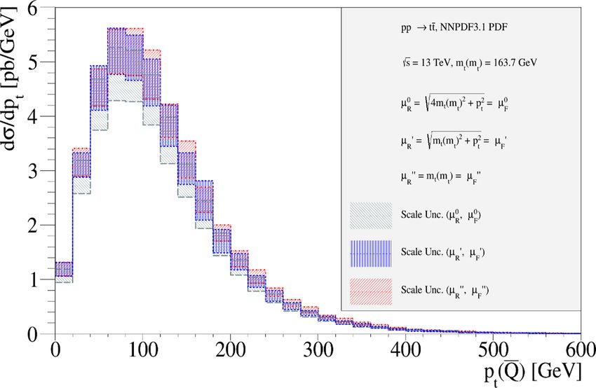
– 25 –Additionally, in this paper we explore the possibility of using a dynamical scale in the
heavy-quark MS mass renormalization, as an alternative to the static value mQ (mQ ) and
its variations used in the previous distributions and in ref. [38]. There, the pT distribution
of the top-quark at NLO was computed for static central scales µR = µF = µm = mt (mt ),
varying them simultaneously by factors 1/2 and 2 around their central value and finding
that the scale uncertainty band was reduced with respect to the case when µR and µF are
varied and µm is fixed to mt (mt ). In general, we expect that dynamical scales, catching the
different kinematics of different events, provide a more accurate description of differential
distributions. Thus, in the following we consider the case when the central values for the
renormalization andq mass renormalization scales are chosen dynamically and coincide, i.e.,
JHEP04(2021)043
µm = µR = µ0 = p2T + 4m2Q (µR ). We fix the central factorization scale to the same
value µF = µ0 . For this configuration, we compute scale uncertainties, by two different
procedures. In the first procedure (i) we fix µR = µm even in the scaleqvariation but we
still vary independently µR in the interval [µR,1 , µR,2 ], where µR,1 = 0.5 p2T + 4m2Q (µR,1 )
q
and µR,2 = 2 p2T + 4m2Q (µR,2 ), and µF in the interval [1/2, 2] around the chosen (mass)
renormalization scale, excluding the (µR , µF ) extreme combinations (2, 1/2) and (1/2, 2),
but keeping all the others, as in the conventional 7-point scale-variation procedure. These
variations implicitly also encode a heavy-quark mass variation, with the mass value span-
ning the interval [m(µR,2 ), m(µR,1 )]. In the second
q
variation procedure (ii), which is more
general than (i), we fix µR = µm = µF = µ0 = p2T + 4m2Q (µm ) in the central predictions
as before, but we vary µR , µF and µm independently from each other, each by factors 1/2
and 2 around µ0 , excluding the extreme scale combinations as in the conventional scale-
variation procedure. In other words, we release the constraint µR = µm during the variation
of these scales. This procedure leads to a 7-point (µR , µF ) scale variation band at fixed
µm (not coinciding with the one of procedure (i), because there the µR = µm scales are
varied simultaneously), and to a more comprehensive 15-point (µR , µF , µm ) uncertainty
band. The pT distributions obtained with the scale configuration and variation procedures
(i) and (ii) are shown in the upper, intermediate and lower left panels of figures 15 and 16
for the charm-, bottom- and top-antiquark, respectively.
For both procedures (i) and (ii), in case of charm, the (µR , µF ) uncertainty band turns
out to be larger than that computed using a fixed value of the charm-mass m qc (mc ) and mak-
ing the standard 7-point scale variation around the central choice µ0 = p2T + 4m2c (mc ),
shown in red in the right upper panel of both figures 15 and 16. Similar considerations on
the size of the uncertainty bands in the comparison between charm results with dynamical
and static scales µm apply also to the 15-point scale variation band, computed according to
procedure (ii) and shown in blue in the left and the right upper panels of figure 16, respec-
tively for the dynamical and static µm cases. In other words, adding µm variations does
not modify the general conclusions inferred by comparing the 7-point uncertainty bands.
On the other hand, in case of top (bottom), close to the peak of the pT distribution,
i.e. in the bulk of the phase-space, the uncertainties accompanying the computation with
dynamical µm are much smaller (smaller) than for µm = mQ (mQ ), as can be seen by
comparing the left and right lower (intermediate) panels of figure 15 for procedure (i)
– 26 –You can also read


