Football analysis using machine learning and computer vision - Filip Öberg Computer Science and Engineering, master's level
←
→
Page content transcription
If your browser does not render page correctly, please read the page content below
Football analysis using machine learning and
              computer vision

                                Filip Öberg

         Computer Science and Engineering, master's level
                              2021

                         Luleå University of Technology
          Department of Computer Science, Electrical and Space Engineering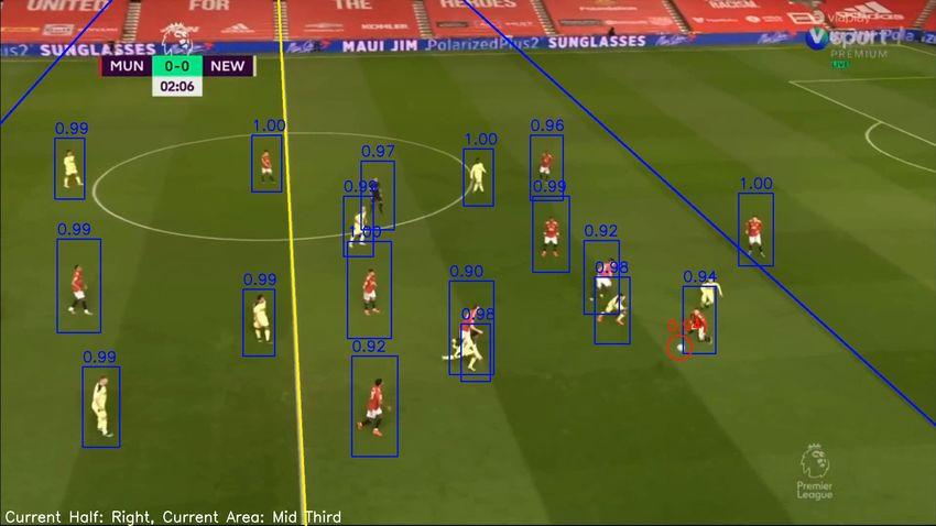
Declaration

I hereby declare that this master thesis has been solely written by me. Any assistance
used from the literature work and books has been referenced with the corresponding
annotations.

Luleå, June 11, 2021                     Filip Öberg
ii

Acknowledgments

I’d like to thank my supervisor Staffan Johansson at Neava for helping me come up with
the idea for this thesis, as well as giving me advice and support from start to end. I’d
also like to thank my internal supervisor Sina for his valuable input relating to my report
and presentation.
Contents

1 Introduction                                                                              2

  1.1   Background & Related Works . . . . . . . . . . . . . . . . . . . . . . . .           2

  1.2   Thesis Objectives & Problem Definition . . . . . . . . . . . . . . . . . . .         4

  1.3   Ethics . . . . . . . . . . . . . . . . . . . . . . . . . . . . . . . . . . . . .     4

  1.4   Delimitation . . . . . . . . . . . . . . . . . . . . . . . . . . . . . . . . . .     4

  1.5   Thesis Structure . . . . . . . . . . . . . . . . . . . . . . . . . . . . . . . .     7

2 Theory                                                                                     8

  2.1   Computer Vision . . . . . . . . . . . . . . . . . . . . . . . . . . . . . . .        8

  2.2   Machine Learning . . . . . . . . . . . . . . . . . . . . . . . . . . . . . . .       9

        2.2.1   Deep Learning and Neural Networks . . . . . . . . . . . . . . . .            9

        2.2.2   Training . . . . . . . . . . . . . . . . . . . . . . . . . . . . . . . .    11

        2.2.3   Convolutional Neural Networks . . . . . . . . . . . . . . . . . . .         13

  2.3   Canny Edge Detection . . . . . . . . . . . . . . . . . . . . . . . . . . . .        13

  2.4   Hough Transform . . . . . . . . . . . . . . . . . . . . . . . . . . . . . . .       17

  2.5   Contour detection . . . . . . . . . . . . . . . . . . . . . . . . . . . . . . .     19

3 Implementation                                                                            22

  3.1   System overview     . . . . . . . . . . . . . . . . . . . . . . . . . . . . . . .   22

                                             iii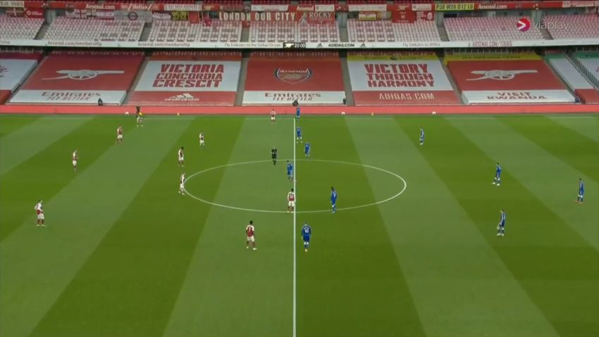
CONTENTS                                                                                 iv

       3.1.1   Configuration and input . . . . . . . . . . . . . . . . . . . . . . .     22

       3.1.2   System loop . . . . . . . . . . . . . . . . . . . . . . . . . . . . . .   23

       3.1.3   Implemented metrics . . . . . . . . . . . . . . . . . . . . . . . . .     38

4 Results                                                                                42

5 Discussion and Conclusion                                                              45

6 Future work                                                                            47

Bibliography                                                                             48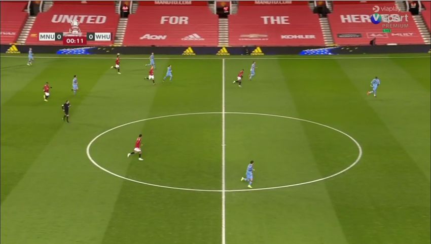
List of Figures

 1.1   Camera angle at the Emirates Stadium . . . . . . . . . . . . . . . . . . .          5

 1.2   Camera angle at Old Trafford . . . . . . . . . . . . . . . . . . . . . . . .        5

 1.3   Example of a correct angle, and an alternate angle from a replay . . . . .          6

 2.1   An example of a fully connected feedforward neural network with two
       hidden layers . . . . . . . . . . . . . . . . . . . . . . . . . . . . . . . . .     9

 2.2   Example of a single neuron in a neural network with inputs, weights and
       activation function. . . . . . . . . . . . . . . . . . . . . . . . . . . . . . .   10

 2.3   The kernels used in Sobel filtering . . . . . . . . . . . . . . . . . . . . . .    14

 2.4   4x5 pixel image with color intensity values . . . . . . . . . . . . . . . . .      14

 2.5   3x3 kernel applied on image . . . . . . . . . . . . . . . . . . . . . . . . .      15

 2.6   Image before and after sobel filtering. . . . . . . . . . . . . . . . . . . . .    16

 2.7   Visualization of double thresholding. The green line will be filtered out
       while the blue line is kept. . . . . . . . . . . . . . . . . . . . . . . . . . .   16

 2.8   Resulting image after all Canny edge detection steps . . . . . . . . . . .         17

 2.9   R-theta parametrization . . . . . . . . . . . . . . . . . . . . . . . . . . .      18

 2.10 Example of a hough space representation of two lines in the image space[32] 19

 2.11 Example of contours and their hierarchy . . . . . . . . . . . . . . . . . .         20

 3.1   Main system loop . . . . . . . . . . . . . . . . . . . . . . . . . . . . . . .     23

 3.2   A detected player with with possession the detected ball . . . . . . . . .         24

                                            v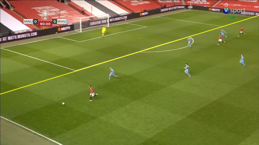
LIST OF FIGURES                                                                             vi

  3.3   Color masking of the red color . . . . . . . . . . . . . . . . . . . . . . . .      25

  3.4   Canny edge detection applied on image with no color filtering . . . . . .           25

  3.5   Canny edge detection applied on image with with color filtering . . . . .           26

  3.6   Non-green colors filtered out to reduce noise . . . . . . . . . . . . . . . .       26

  3.7   Canny edge detection applied on an image frame . . . . . . . . . . . . . .          27

  3.8   A detected line on the halfway line . . . . . . . . . . . . . . . . . . . . .       28

  3.9   The detected line is extended to the edges of the screen . . . . . . . . . .        28

  3.10 Non-green colors filtered out to reduce noise . . . . . . . . . . . . . . . .        29

  3.11 Canny edge detection applied on an image frame . . . . . . . . . . . . . .           30

  3.12 A detected line on the box line      . . . . . . . . . . . . . . . . . . . . . . .   31

  3.13 The detected line is extended to the edges of the screen . . . . . . . . . .         31

  3.14 The detected halfway line is translated to act as boundaries for the middle
       third . . . . . . . . . . . . . . . . . . . . . . . . . . . . . . . . . . . . . .    32

  3.15 The detected penalty box line is translated to act as a boundary between
       the right and middle third . . . . . . . . . . . . . . . . . . . . . . . . . .       33

  3.16 One of the halves of the centre circle detected, with the extreme points
       marked with blue circles. . . . . . . . . . . . . . . . . . . . . . . . . . . .      34

  3.17 Attack zone boundaries approximated with the help of contour extreme
       points . . . . . . . . . . . . . . . . . . . . . . . . . . . . . . . . . . . . .     35

  3.18 Penalty box semi-circle detected, with topmost and bottommost points
       marked with blue circles. . . . . . . . . . . . . . . . . . . . . . . . . . . .      35

  3.19 Attack zone boundaries approximated with the help of contour extreme
       points . . . . . . . . . . . . . . . . . . . . . . . . . . . . . . . . . . . . .     36

  3.20 Flowchart describing the logic of determining the half and third the ball is
       in . . . . . . . . . . . . . . . . . . . . . . . . . . . . . . . . . . . . . . . .   37

  3.21 Ball position by halves . . . . . . . . . . . . . . . . . . . . . . . . . . . .      39

  3.22 Action zones . . . . . . . . . . . . . . . . . . . . . . . . . . . . . . . . . .     39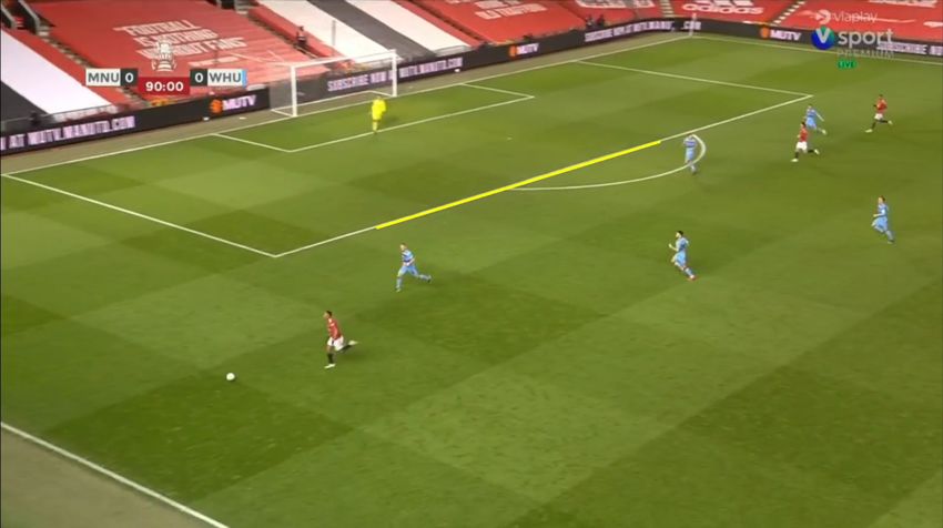
LIST OF FIGURES                                                                           vii

  3.23 Ball possession . . . . . . . . . . . . . . . . . . . . . . . . . . . . . . . .    40

  3.24 Ball possession split in 5-minute periods . . . . . . . . . . . . . . . . . .      40

  3.25 Attack zones . . . . . . . . . . . . . . . . . . . . . . . . . . . . . . . . . .   41

  5.1   A bounding box with players from both teams within it . . . . . . . . . .         45
List of Tables

 4.1   Comparing ball possession statistics . . . . . . . . . . . . . . . . . . . . .   43

 4.2   Comparing action zones statistics . . . . . . . . . . . . . . . . . . . . . .    43

 4.3   Comparing attack zones statistics . . . . . . . . . . . . . . . . . . . . . .    43

                                          viii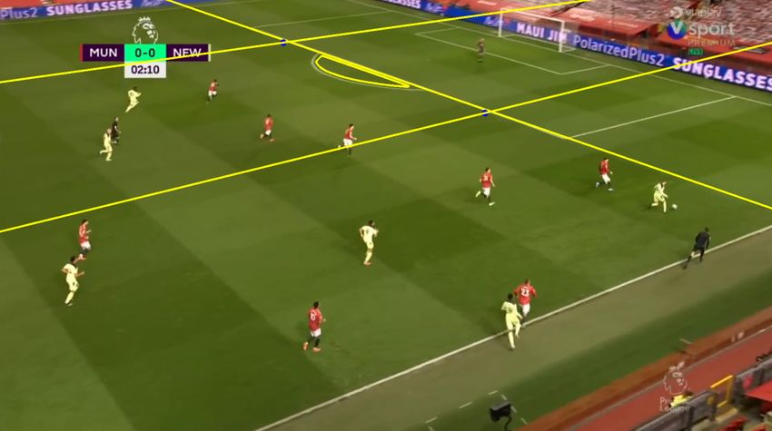
Abstract

The industry of football analysis and football statistics is a booming one. Most profes-
sional football teams these days make use of sophisticated tools and systems that analyze
their training, their games, and their players in every way possible. More and more de-
cisions are built on what the data and these system says. However, these systems are
expensive and require wearable devices that determine the players positions and other
performance metrics. This thesis presents a tool that makes use of machine learning and
computer vision techniques to automatically extract football statistics and football data
from video recordings from a single camera, without any other devices or data collecting
sensors. The output of the tool is then compared to the same metrics and statistics that
are being tracked on popular football statistics websites. The system has been tested on
video recordings from two different stadiums and has produced results that differ only by
1-5 percentage points from the established statistics sources when comparing the "Action
zones" metric and ball possession. The "Attack zone" metric produces much more var-
ied results, differing by 0-21 percentage points when comparing to established statistics
sources.

                                           1
1 Introduction
Sports statistics and analysis is a huge industry and is growing steadily every year [1].
Sports teams and organizations in all kinds of different sports, professional or amateur,
are making use of performance data and analytic tools to gain insight into how to improve.
It can assist in making decisions around player development and recruitment, training
and rehabilitation programs, tactics, and more.
Like with most systems these days, these analytic tools depend on having data that
they can analyze. The analysis is only as good as the data it consumes. Data collection
is usually done with several cameras, wearable sensors, combined with the help of GPS
or other positioning technologies [2].
However, data collection can be expensive. The more sophisticated the tools get, the
more expensive and complicated they become. Which also means that they become less
available for smaller teams and organizations.
This thesis report presents a tool that can extract football statistics from a football
game that has been recorded using only a single camera. No other hardware or sensors
are needed. The tool has been tested on recordings of professional football games, and
the resulting statistics are then compared to statistics available from popular and estab-
lished football statistics sources. This tool can then potentially provide smaller teams
and organizations with statistics from their games, which could give them more insight
into how their games play out.
1.1 Background & Related Works
To be able to produce information about a game of football, you need to be able to
detect the positions of the players and the ball, as well as where they are located on
the playing field. Everything that happens in a football game, in terms of statistics and
performance metrics, revolves around the players, the ball, and their respective positions
on the playing field.
2CHAPTER 1. INTRODUCTION 3
Object detection is one of the biggest and most important branches of the computer
vision field [3]. It has a wide variety of applications and is prominent in many shapes in
everyday life, ranging from detecting obstacles in autonomous vehicles, to face detection
and facial recognition.
The last decade has seen major breakthroughs in the areas of generic object detection
[4], and there are now a wide variety of generic object detectors that can be used to
build applications where object detection and recognition are needed [3]. The definition
of generic object detection is determine whether there are instances of objects from pre-
defined categories present in an image, and where in the image these objects are located.
The amount of predefined categories are usually large, so a generic object detector has
to be able to detect a wide variety of objects in an image.
However, for the scope of this thesis, detection of a large amount of different object
categories is not required, since the only objects that has to be detected are the players
and the ball. Luckily, more specialized methods for detection of balls and players has
been proposed in recent years. Speck et al (2017)[5], and Gabel et al (2019)[6] both
proposes methods using convolutional neural networks for detecting the ball in games
from the RoboCup, an annual robot football competition [7]. However, these solutions do
not detect the players, and the camera angles and the relative size between the ball and
the players are not the same as in the long distance shots and angles that are within the
scope of this thesis.
Komorowski et al’s (2020)[8] FootAndBall detector however, is another convolution
neural network based solution specifically designed for detecting both football players
and the football in the long distance shots we work with within this thesis. This is the
detector chosen for the player and ball detection in this thesis.
The positions of the players and the ball is not enough to generate any meaningful
data or statistics from a game of football. Further analysis has to be done with the
information gained from the detector. Beetz et al (2005)[9] uses the position of the ball
and the players to determine if the ball is being passed, dribbled, or just kept in possession.
The positional data is also used to identify typical situations, such as a counter-attack, or
strictly possession-based attacks. However, this system uses tiny microwave senders in the
players shin pads and in the ball to determine their positions, whereas this project only
has video recordings from a single camera to work with, no other sensors or hardware.CHAPTER 1. INTRODUCTION 4
1.2 Thesis Objectives & Problem Definition
The problem that this thesis deals with is the problem of unsupervised and automatic
analysis of a game of football and generating statistics based on the events occurring
on the field of play. More specifically, to investigate to what extent this can be done by
developing a tool that can analyze a video recording of a football game and automatically
generate football statistics by recognizing the ball, the players, and other important areas
of the field during the match. The input to the system will be a video recording of a
football game. The system then uses a machine learning algorithm together with computer
vision techniques to detect the ball, the players, and other important areas of the field.
The players are also separated between the two playing teams. Combined, this will give
the tool the ability to determine if the ball is or isn’t in a certain area of the playing field,
which team that has possession of the ball, and what areas of the field that the ball has
been in the most over the course of the game.
1.3 Ethics
The data generated by the tool developed in this thesis is not shared or uploaded to any
third party and the user has full control of the data and what to do with it. This tool
is an alternative to other commercially available analytic tools that make use of more
advanced methods of data collection, such as GPS trackers. The data collected by these
analytic tools may or may not be shared or sold to third parties.
None of the data generated by this tool is personal and it cannot be used to identify a
single person. However, the tool uses video recordings of football games as input. These
recordings contain images of people, which might be considered personal data. If that’s
the case, measures might have to be taken to comply with GDPR.
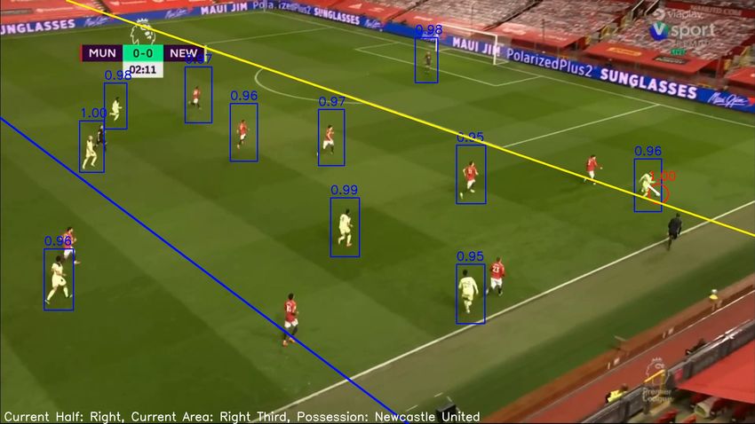
1.4 Delimitation
During development and testing, footage from professional football games from the En-
glish top division have been used as input. The different stadiums these games are played
in have different layouts and have the main camera mounted at different heights and an-
gles. The orientation of the field in the recorded footage is therefore different depending
on the stadium, and angles are something that needs to be accounted for when it comes
to detection of features of the playing field. The lighting is also different from stadium to
stadium. Therefore, to make testing and development more consistent, only footage fromCHAPTER 1. INTRODUCTION 5
two specific stadiums have been used. These stadiums are the Emirates Stadium [10] and
Old Trafford [11]. See figure 1.1 and figure 1.2 for examples of the camera angle at these
stadiums.
Figure 1.1: Camera angle at the Emirates Stadium
Figure 1.2: Camera angle at Old Trafford
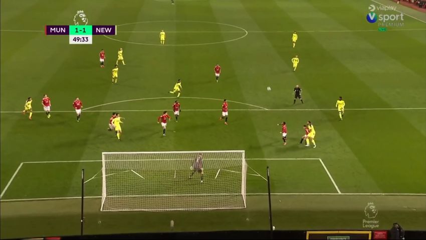
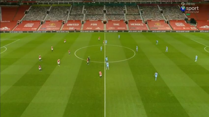
TV recordings of football games contain replays and frames filmed from an alternate
angle (closeups, frames from a different camera, and so on). The problem definition andCHAPTER 1. INTRODUCTION 6
the scope of the project says that the recordings are only from a single camera and a
single camera angle. However, to save time, these replays and alternate angles are kept
in the input recordings anyway. Some efforts have been taken to filter these frames out
when running the program, such as ignoring frames where there is not enough green in
the center of the image (no grass), but it is not completely robust. The amount of frames
that comes from replays and other angles are very small in comparison to the amount of
frames that are from the "correct" angle. So the results will not vary that much because
of this. An example of a correct and incorrect camera angle can be seen in figure 1.3
Figure 1.3: Example of a correct angle, and an alternate angle from a replayCHAPTER 1. INTRODUCTION 7 1.5 Thesis Structure The thesis is structured as following: Chapter 2 briefly covers and explains the methods and techniques used to solve the problems presented in the 1.2 section. This is to make it easier to follow and understand what is being done in the 3 chapter. Chapter 3 explains more in detail how the system is built and implemented. It gives an overview of how the system is configured and set up, and then explains how every step in the system loop/pipeline works and how it has been implemented with the methods mentioned in the 2 chapter. Chapter 4 presents the results of the system, i.e the output in the form of the football statistics that the system generates after it has finished analyzing the recording of the football game. Chapter 5 then discusses the results and investigates if the problem originally presented in the 1.2 has been solved, and to what degree. Lastly, chapter 6 briefly mentions how the system can be improved and built upon in the future.
2          Theory

This chapter will give a brief introduction to the different scientific techniques and meth-
ods used in this thesis. It will give you as a reader a better understanding of the imple-
mentation as well as the result that it produces. The chapter will go through some basic
theory in computer vision, machine learning and neural networks. The specific computer
vision techniques and methods used in the implementation of this project will also be
explained here.

2.1          Computer Vision

Computer vision is a scientific field that deals with how computers can gain an under-
standing and retrieve information from digital images. It aims to mimic the human visual
system and automate tasks that would normally require human visual inspection [12].
The domain of computer vision includes the fields of object detection and feature ex-
traction [13]. Both object detection and feature extraction are techniques that are used
extensively in this thesis for detecting the players and the ball, as well as detecting the
features of the playing field, such as the lines in the grass.

    Object detection can be achieved in numerous ways. In this thesis, a machine learn-
ing algorithm is used. The advantage of using a machine learning algorithm for object
detection is that the algorithm can learn on its own how to identify an object and what
features to look for in an object by observing a dataset of images where the location
of the specific objects are given. Traditionally, the features to look for (i.e a square has
four corners, the cat is black and has four legs, etc) would first have to be manually
defined for every object that you wish to be able to detect. And secondly, the methods
to detect these features would have to be manually implemented using techniques like
edge detection, corner detection or threshold segmentation [14]. Feature extraction, more
specifically edge detection and line extraction, is achieved by using techniques and meth-
ods implemented in the OpenCV1 library. Explanations on how these methods work are
    1
        www.opencv.org

                                             8
CHAPTER 2. THEORY 9 provided later on in this chapter. 2.2 Machine Learning Machine learning is a subfield of the larger Artificial Intelligence field [15]. Arthur Samuel in 1959 defined machine learning as the field of study that gives computers the ability to learn to do things without being explicitly programmed to do so [16]. This thesis takes advantage of an algorithm that uses the "Deep learning" approach to training a neural network[8]. 2.2.1 Deep Learning and Neural Networks Deep learning is a family of machine learning methods that makes use of an "Artificial Neural Network" (ANN), more commonly referred to as just "Neural Network" (NN), for training of the algorithm. A common type of neural networks are the feedforward neural networks, also known as a Multilayer Perceptron [17]. The neural network is inspired by the structure of the human brain, with its neurons and synapses, hence its name. Figure 2.1: An example of a fully connected feedforward neural network with two hidden layers A feedforward neural network, as seen in figure 2.1, consists of one input layer, one output layer, and one or several hidden layers of interconnected nodes or "neurons". Each neuron consists of an Activation or Transfer function and a series of weights, with one weight associated with every incoming connection. When a value gets passed through one
CHAPTER 2. THEORY 10
of the incoming connections, the value gets multiplied with the weight of the connection.
The weighted values of all incoming connections are then summed up, and passed into
the Activation function.
Figure 2.2: Example of a single neuron in a neural network with inputs, weights and
activation function.
As seen in figure 2.2, s is the sum of each of the inputs xi multiplied by its corre-
sponding weight wi :
N
s= (2.1)
X
wi x i
i=1
And the sum s is then passed into the activation function to produce the output of the
neuron y:
y = f (s) (2.2)
These weights are initialized to random values at first, but are continuously tweaked
and changed during the training of the neural network. These weights together with the
activation function determine the relation between the input and the output of the neural
network. The activation function is chosen beforehand and is not changed during training.
Two commonly used activation functions are the sigmoid function, seen in 2.3 and the
ReLu function, seen in 2.4.
1
f (s) = (2.3)
1 + e−s
s
if s ≥ 0
f (s) = max(0, s) = (2.4)
0
if s < 0
Both the sigmoid function and ReLu function are non-linear, which is important
because if the neural network is to be able to solve non-linear problems, it needs to
have a non-linear relationship between the inputs and outputs. The sigmoid function also
outputs a value between 0 and 1, which is good for Classification problems.CHAPTER 2. THEORY 11
2.2.2 Training
Training a neural network is all about finding the set of weights that produce the best
output accuracy from the neural network. There are various ways that this can be done.
The method that is most relevant to this thesis is the method of supervised learning. In
supervised learning, the neural network learns by examining a set of labeled training data.
Depending on what type of data the neural net is trained on, the labels can be different
things. If for example the neural net is predicting the positions of cats in an image, the
labels are the actual positions of the cats in an image. This way, the neural net can
make predictions on the set of training data, and then compare the predictions with the
labels to see how accurate the predictions were. The way the accuracy is measured is by
calculating the loss. Loss is the penalty for a bad prediction, so the aim during training
of the neural network is to minimize loss as much as possible. The loss is calculated with
a loss function, of which there are many to choose from, depending on the circumstance.
The method used to minimize the loss function is called the optimization algorithm [18].
Loss functions
Loss functions, roughly speaking, can be of two types: Classification and Regression loss
functions [19, 20]. Regression loss functions are used when the neural net predicts a
quantity, for example the price of a house. While classification loss functions are used
when the neural net is predicting labels, like detecting what kind of objects are in an
image [21]. A popular and very simple classification loss function is the Mean Square
Error loss function, also known as MSE. MSE is simply the average sum of squared
distances between the predicted value and the actual value (the label).
1 XN
M SE = (label − prediction)2 (2.5)
N i=1
The smaller the difference between the label and the prediction, the smaller the loss
will be. Minimizing loss therefore means maximizing the accuracy of the predicitons.
When it comes to classification, the neural net will output a confidence value between 0
and 1 on every neuron in the output layer. Each output neuron represent a decision or a
choice and the value is how confident the neural net is in that decision. For example, a
neural net that recognizes numbers will output how confident it is that the image contains
a certain number. If the neuron that represent the numbers 9 and 2 has the confidence
0,2 and 0,9 respectively, then the neural net is more confident that the image contains
a 9 rather than a 2. For this, a loss function that outputs a value between 0 and 1 is
needed. A popular choice is the Cross-Entropy loss function, which comes in two shapes,CHAPTER 2. THEORY 12
the binary or non-binary version. Which one to use depends on if the classification is
binary, i.e "Does this image contain a cat or not", or non-binary, i.e "What kind of cat is
this?". The Cross-Entropy loss function is defined as:
n
LCE = − ti log2 (pi ) (2.6)
X
i=1
Where ti is a binary indicator (0 or 1) that tells if the class i (i.e type of cat) is the
correct classification for the current observation, and pi is the neural networks confidence
that it is. This loss function is logarithmic and the loss function heavily penalizes confident
wrong predictions.
Optimization
Intuitively, one way to minimize loss would be to, for every weight parameter w in the
network, plot the relationship between the value of the weight and the loss from the loss
function. This resulting plot would have a global, and possibly multiple local minima.
If the weight value that corresponds to the global minimum was picked for every single
weight parameter, it would result in an optimized network. Calculating this for every
weight parameter and for every possible value of each weight is not feasible. A popular
approach is instead to make use of Gradient Descent. Like the name suggests, gradient
descent means gradually reducing loss by descending down the curve. The slope of the
curve can be calculated with its derivative, the weights are then updated in the direction
of the negative slope. How much the weights are being increased/reduced is another
parameter called the Learning Rate.
The learning rate is important because a balance has to be found between fast conver-
gence towards the minimum, while still avoiding overshooting, which is when the learning
rate is too large and causes the descent to miss the minimum by jumping over it back
and forth.
There are several other algorithms and other types of gradient descent methods (Like
the popular Stochastic Gradient Descent), depending on how the training data is split up
and how often the weights gets updated, but the general idea of how they work are the
same [18].CHAPTER 2. THEORY 13
2.2.3 Convolutional Neural Networks
This section will briefly cover Convolutional Neural Networks which is a kind of Neural
Network that specializes in images and takes an image as input instead of other values.
This is the kind of network that is used in this thesis for object detection.
Convolutional Neural Networks (CNNs) are a subclass of the Artificial Neural Network
(ANN) covered earlier. What differs between the two is that, in addition to the fully
connected layers (which is the only layer that the traditional ANN has), a CNN has
Convolutional layers and Pooling layers. The whole idea of these layers is to reduce
complexity in the network. If an image were to be fed into a regular ANN where each
pixel corresponds to one input neuron (or three neurons, if its an RGB color picture,
one for each color), and the hidden layers are all fully connected to one another, the
amount of weights would be incredibly large and it would simply be too complex for a
regular computer to handle [22]. When training a CNN, the same principles of reducing
loss applies. In the case of training for detection of a certain object, the input training
data are images and the labels are instead areas of the image where the object is present.
2.3 Canny Edge Detection
The Canny edge detection algorithm was published in 1986 by John Canny[23], and is still
one of the most widely used edge detectors today. Essentially, the Canny edge detection
algorithm is done in four steps: Gaussian filtering (blurring, essentially), Sobel Filtering,
non-maximum suppression and lastly hysteresis thresholding[24].
The Canny edge detector can be seen as an optimizer of the Sobel filter, as it takes a
Sobel filtered image as an input and outputs an image with clear and less noisy lines. The
Sobel filter, also known as the Sobel operator, works by "scanning" an image in the x and
y direction with a 3x3 kernel. When the image is scanned in a sliding window manner
with the 3x3 kernel, edges can be detected by finding sharp increases in color intensity
within the 3x3 pixel grid. The two kernels that are used can be seen in figure 2.3 [25]:CHAPTER 2. THEORY 14
Figure 2.3: The kernels used in Sobel filtering
As an example, consider figure 2.4 representing a 4x5 pixels image, with each number
representing the color intensity in that pixel.
Figure 2.4: 4x5 pixel image with color intensity values
Clearly, there is a change in intensity between the second and third pixel in the x-
direction. Now, the kernel is applied on these highlighted pixels in figure 2.5:CHAPTER 2. THEORY 15
Figure 2.5: 3x3 kernel applied on image
Using the kx kernel seen in 2.3, a sum is calculated by summing up the product of
the pixel intensity and the corresponding position in the kernel:
Gx = 50×(−1)+50×(−2)+50×(−1)+50×0+50×0+50×0+100×1+100×2+100×1 = 200
(2.7)
The higher the sum, the larger the difference in intensity is, which means that there is
a higher chance of an edge here. If there were no change in intensity (i.e, if the intensity
was 50 in all pixels) the sum would cancel out and result in 0. This is the case if the ky
kernel is used instead, since there is no edge in the y-direction:
Gy = 50×1+50×2+100×1+50×0+50×0+100×0+50×(−1)+50×(−2)+100×(−1) = 0
(2.8)
When the 3x3 area has been scanned in both directions, the magnitude of the edge
M and the orientation θ can be calculated with equations 2.9 and 2.10, respectively:
q
M= G2x + G2y (2.9)
Gy
θ = arctan( ) (2.10)
GxCHAPTER 2. THEORY 16
Figure 2.6: Image before and after sobel filtering.[26, 27]
The result of the Sobel filter on a complete image can be seen in 2.6. Notice that
there is an abundance of lines being detected and a lot of "noise" showing up as white,
i.e areas that really shouldn’t be considered a line. There’s also a lot of thick lines, which
are the lines that had the greatest magnitude. Thin lines are preferred as it gives a better
idea of where the edges are and gives a clearer outline of the object. This is where the
non-maximum suppression step comes in.
Non-maximum suppression works by only keeping the brightest pixel of each edge.
For example, if an edge is three pixels wide, and has a gradient where the middle pixel
is the brightest and the two neighboring pixels are less so, only the brightest pixel (with
the greatest magnitude) is kept while the other pixels are blacked out. This removes a
lot of the gradient edges seen in 2.6 and produces thinner lines.
Figure 2.7: Visualization of double thresholding. The green line will be filtered out while
the blue line is kept.
The last step of the algorithm is the Hysteresis Thresholding, or Double Threshold
step. This last step is for filtering out the last remaining lines that might come from color
variation and noise. Like the name suggests, two magnitude thresholds are defined, as
seen in figure 2.7. The lower threshold defines the minimum magnitude of a pixel for it toCHAPTER 2. THEORY 17
still be considered as part of an edge. The upper threshold sets the minimum magnitude
for a pixel to always be considered as part of an edge. If a pixel magnitude falls in between
these thresholds, the pixel is only kept if that pixel is part of an edge that has pixels with
magnitude above the upper threshold. In short, every pixel below the lower threshold gets
filtered out, every pixel above the upper threshold is kept, and every pixel in between the
thresholds are kept if it is connected to other pixels that are above the upper threshold,
and gets filtered away otherwise.
Figure 2.8: Resulting image after all Canny edge detection steps [28]
The final result can be seen in 2.8. Here, a lot of noise and detail has been filtered
away but most of the edges that define the object is still intact.
2.4 Hough Transform
The Hough Transform is a method for extracting features from a binary image. The
original proposition from 1962 by Paul Hough was designed to detect and extract lines[29],
but has since then been extended to be able to detect other shapes, for example circles[30].
This section will briefly explain how the Hough transform detects lines, which is the
use case it has in this thesis. A straight line can be represented mathematically in many
ways, the most common being:
y = mx + b, (2.11)
where m is the slope of the line, and b is the point where the line intercepts the y-axis.
However, for completely vertical lines, m would be unbounded. To tackle this, it was
proposed to use the Hesse normal form for representing lines in the Hough transform[31]:
r = xcosθ + ysinθ (2.12)CHAPTER 2. THEORY 18
Figure 2.9: R-theta parametrization
As seen in figure 2.9, a line can be completely defined by the two parameters r and
θ, where r is the distance from the origin to the closest point on the line, and θ is the
angle between that perpendicular line connecting the origin and the closest point of the
line and the x-axis. The line can therefore be represented as a single point, (r, θ), in a
Parameter Space with the axis of θ and r, also called the Hough Space.
When detecting lines with Hough transform, one would usually run the image through
an edge detection algorithm before so that only the edges in the image is left. Then,
every pixel of the remaining edges are scanned. A pixel is a single point in the image
space, and can have an infinite amount of lines passing through it. Remember that a
line is represented as a single point in Hough space. Turns out that if you would take
into account all of these potential lines passing through a single point, it would form a
sinusoidal in the Hough space, so a pixel in the image space is a sinusoidal in Hough
space. When all pixels have been analyzed, the Hough space will be filled with a lot
of sinusoidals, overlapping. Each intersection can be seen as a vote for a line. Since an
intersection point in the Hough space can be translated back to a straight line in the
image space, several sinusoidals that intersect in the same point means that there are
several pixels in the image space that has the same line passing through them.CHAPTER 2. THEORY 19
Figure 2.10: Example of a hough space representation of two lines in the image space[32]
In 2.10 you can see two bright spots in the hough space graph where a large amount
of sinusoidals have intersected. The brighter the points, the more "votes" has been cast
in favor of that line. When using an implementation of the Hough transform, like in
OpenCV, one would set a minimum threshold value which filters out lines that doesn’t
have enough votes.
When the scan has been complete, you can extract the line by taking the brightest
spots in the Hough space, and finding the corresponding (r, θ) pair and putting it in
equation 2.12. In a real implementation the votes are saved in accumulators in a 2-d
matrix/array where the matrix position represents the r and θ.
A Probabilistic Hough Transform is a version of the Hough transform algorithm where
not all edge points are used, but instead picks a set of random edge points from the image.
The probabilistic approach was proposed by Kiryati et al [33] and it turns out that the
accuracy of the algorithm remained high even when using just a small percentage of edge
points picked at random, but with significant gain in execution time. The probabilistic
hough transform implemented in the OpenCV library is the variant that is being used in
this thesis.
2.5 Contour detection
Another common computer vision method used in the thesis is the method of finding and
extracting contours in an image. A contour is the border which completely surrounds anCHAPTER 2. THEORY 20
area in an image. Finding contours can be very useful when trying to find objects and
features in an image.
Once again, the OpenCV library is used for finding contours in this project. The
OpenCV library implements a contour finding algorithm proposed by Suzuki et al [34] in
1985, also known as Suzuki’s algorithm. This section will briefly explain how it works.
Figure 2.11: Example of contours and their hierarchy
Suzuki’s algorithm finds both the inner and outer contours, or boundaries, when
scanning an image. The algorithm also keeps track of the hierarchy of the contours, i.e if
a contour is completely enclosed by another, and so on. An example of borders and their
hierarchy can be seen in 2.11. The input to the algorithm is a binary image, i.e an image
where the value of a pixel is either 0 or 1, which means that an image that has been fed
through the Canny edge detection algorithm would work very well in this case.
The algorithm works by scanning the image from left to right, top to bottom, and
when it finds a pixel which value is 1 (i.e not the same value as the background, which is
0), it sets that pixel as a starting point for the traversal of the possible contour. It then
scans the neighboring pixels to find another pixel which has the same value, sets that
pixel as a new starting point, and so on. When the algorithm has reached back to the
initial starting point, it stops, and it has now found the whole contour. Every pixel that
is part of this contour has been labeled a number, this is to keep track of the different
contours. This is also useful for building the contour hierarchy, since the algorithm also
keeps track of which outer border/contour it has last encountered, which will be the the
parent contour of any possible new contours found within. Referring back to 2.11 again,CHAPTER 2. THEORY 21 where Inner Border 1 (ib1), Inner Border 2 (ib2) are children of their parent contour, Outer Border 1 (ob1).
3       Implementation

3.1      System overview

The system is making use of the FootAndBall player and ball detector[8]. The detector
takes an image as an input and returns coordinates for bounding boxes for the detected
players, and a coordinate for the detected ball. It also returns a number together with
each detection that represent how confident the algorithm is that the detection is correct.
After the players and the ball has been detected, the same image gets passed into several
other stages where more work is done to detect other things and features. More details
are provided in the System loop section

3.1.1     Configuration and input

Before the system is run some configuration is required. This is done in a config file that is
passed on into the program when run. The most important parameters that are specified
are:

    • Path to the weights of the FootAndBall neural network

    • Path to the input video files

    • Names of the competing teams

    • RGB value of a color that can uniquely identify one of the teams

    • Which team that has the unique color (Home or Away)

    • Which team that starts the game from the left half of the field (Home or Away)

    • Output type (Realtime, video file, or none)

    • Filename of the output video file, if needed

                                             22
CHAPTER 3. IMPLEMENTATION 23
The weights of the neural network are generated when the network is trained. The
FootAndBall model comes pre-trained on two large datasets. However, more training had
to be done to get satisfactory detection levels on the recordings that has been used during
development and testing. Manual annotation has been done on footage from other games
from the English Premier League, and the model has been trained with this additional
dataset.
The input to the system are two video files, one of each half of the game. Ideally, the
recordings should be from a single camera, so if the recordings are of a TV-broadcast,
replays and closeups should be trimmed away. The system can cope with closeups to a
degree, because the players and ball will be too large for the neural network to detect, and
there will rarely be a line that is detectable. Replays, however, can cause be problematic
with the alternative angles that can cause the system to think it’s in the wrong half, not
to mention that it will count possession and other metrics during the replay. The impacts
from the replays have proven to be minimal during testing, but to get the most accurate
results, replays should be avoided.
A unique color of one of the teams is also specified in the config file, as well as which
team the unique color belongs to. This is needed for team recognition purposes.
Which team that is starting from the left (from the viewpoint of the camera) needs to
be known to correctly add up the different metrics over the two halves, since the teams
change half after halftime.
There are three different output types from the system. "Realtime", which outputs a
video stream in realtime while the system is running, this is good for debugging. No video
file is generated. "Video", generates no realtime output, but instead generates a video file
with the output. Lastly, "None", generates no video output and only outputs the finished
statistics at the end. If "Video" output is chosen, the name of the video file is specified in
the config file as well.
3.1.2 System loop
Figure 3.1: Main system loopCHAPTER 3. IMPLEMENTATION 24
After the configuration is done and the program has been initialized, the program enters
the main system loop, seen in figure 3.1. This is where the bulk of the work is done. The
loop is implemented in several steps, and each frame of the input video is fed through
these steps. Each step has a defined purpose.
Player, team, and ball detection
The first step is the player and ball detection through the FootAndBall neural network.
This returns coordinates for the bounding boxes around the detected players, as well as
the coordinate for the detected ball. The ball coordinate is then used in the subsequent
steps to determine which area of the field the ball is in. Another thing that is being done
in this step is to determine which team that has possession of the ball. The assumption
here is that the player that is closest to the ball is the player that has possession.
First, the closest player is found by finding the smallest distance between the centre
point of the bounding boxes and the ball. Figure 3.2 shows a player that has been detected
as being the closest player to the ball.
Figure 3.2: A detected player with with possession the detected ball
When the closest bounding box has been found, the area within the box is analyzed
to determine which team the player belongs to. This is done with color masking through
the OpenCV library. A color range in the HSV color space is created based on the unique
color defined in the config file. The image is then filtered with this color range in mind.CHAPTER 3. IMPLEMENTATION 25
Figure 3.3: Color masking of the red color
In figure 3.3, the colors that are within the color range turn white, while all other
colors turn black. The white pixels are then counted and if the count exceed a certain
threshold, then it’s determined that the player belongs to the team with the unique color.
If the threshold is not exceeded, the player is assumed to be in the other team.
Halfway line detection
The first step of any line detecting step is to filter out any part of the frame that isn’t the
playing field. This is done by filtering out any color that is not considered a shade of green.
This helps to stop edges being detected from areas up in the stands when applying the
Canny edge detecting algorithm. This is especially a problem now during the pandemic,
where the stands are empty and lots of straight lines are present in those areas. The
difference can be seen in figure 3.4 and figure 3.5:
Figure 3.4: Canny edge detection applied on image with no color filteringCHAPTER 3. IMPLEMENTATION 26
Figure 3.5: Canny edge detection applied on image with with color filtering
First, the color filtering is applied in figure 3.6:
Figure 3.6: Non-green colors filtered out to reduce noise
The next step is to apply the Canny edge detection algorithm on the filtered frame,
as seen in figure 3.7CHAPTER 3. IMPLEMENTATION 27
Figure 3.7: Canny edge detection applied on an image frame
A probabilistic Hough transform is then applied on this to extract the lines of the
image. The Hough transform takes a few parameters as input, such as minimum length
of a line, as well as how large a gap in a line can be while still being considered the same
line, and so on. The Hough transform returns all detected lines that have been detected
within the frame of the input parameters. The next step is to filter out all the lines that
aren’t the halfway line. The halfway line is the only line in the frame that is vertical
(within a few degrees), so by checking the angle of the lines, a good candidate for the
halfway line can be found.CHAPTER 3. IMPLEMENTATION 28
Figure 3.8: A detected line on the halfway line
The line in figure 3.8 is then extended to the edges of the frame in figure 3.9. This
is to enable translating and rotating of the line when the boundaries for the thirds are
approximated. See Thirds approximation ("Action Zones") for details. This line is then
used to determine which half the ball currently is in.
Figure 3.9: The detected line is extended to the edges of the screenCHAPTER 3. IMPLEMENTATION 29
Penalty box line detection
The detection of the penalty box line (The line parallel to the extended goal line) is done
in similar fashion to the halfway line detection.
First the non-green color filtering is applied on the filtered frame in figure 3.10.
Figure 3.10: Non-green colors filtered out to reduce noise
Then, the Canny edge detection algorithm is applied in figure 3.11.CHAPTER 3. IMPLEMENTATION 30
Figure 3.11: Canny edge detection applied on an image frame
The Hough transform is then applied once again to extract the lines of the image.
Just like in the halfway line detection, an angle interval is used to filter out the lines
that are not wanted. The angle of the box line is different depending on which side of the
field the camera is pointing, so this interval is different depending on which half of the
field the camera is pointing towards.
Since there are more lines that have the same angle as the box line, some more filtering
needs to be done. In this case, the line that is furthest to the center of the field is the line
that is most likely to be the box line. In the above example, the line that fall within the
angle interval, and is furthest to the right, is most likely the box line.CHAPTER 3. IMPLEMENTATION 31
Figure 3.12: A detected line on the box line
This line in figure 3.12 is then extended in figure 3.13 for the same reasons, to make
translation and rotation possible when approximating the thirds. See Thirds approxima-
tion ("Action Zones") for details.
Figure 3.13: The detected line is extended to the edges of the screenCHAPTER 3. IMPLEMENTATION 32
Thirds approximation ("Action Zones")
"Action zones" is a common statistic that tells you how much of the time the ball has
been spent in a certain third of the field. I.e the left, middle, or right third. To be able to
do this, boundaries between these thirds has to be determined. The way these boundaries
are found are by translating and rotating the already detected halfway line or penalty
box line, depending on which one of these are visible at the time. The translation is done
by rotating the detected halfway line or penalty box line to create a translation vector.
The start and end points of the line is then translated along this translation vector. The
translation vector is also scaled so that it is of the desired length for the translation.
If the halfway line is visible, it gets translated in both directions to act as bound-
aries for the middle third. The lines are also rotated slightly to better follow the actual
orientation of the field. This can be seen in figure 3.14.
Figure 3.14: The detected halfway line is translated to act as boundaries for the middle
third
If instead the penalty box line is visible, that line gets translated towards the middle
of the field. This line is also rotated to account for the orientation of the field, as seen in
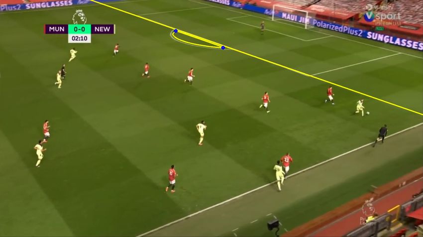
figure 3.15.CHAPTER 3. IMPLEMENTATION 33 Figure 3.15: The detected penalty box line is translated to act as a boundary between the right and middle third Attack zone approximation "Attack zones" is another common statistic that tells you which "corridor" each team has used the most when attacking towards their opponent’s goal. The "corridors" are usually the respective teams left and right wing, as well as the centre of the field. This means that boundaries between these corridors has to be approximated. This is similar to the "Action zones" boundaries, i.e splitting up the field in thirds, but this time the boundaries are parallel to the length of the playing field. This is a bit more complex than the case of the "Action Zones", since there are no lines in the horizontal direction that are visible in the frame most of the time. Instead, the approach is to make use of the already detected penalty box line or halfway line together with the contour of the centre circle and the half-circle outside the penalty box. Similarly to the Action Zone approximations, there are two cases to take into account. One case when the halfway line is visible, and one case where the penalty box is visible. And like in all the previous detection steps, green filtering and canny edge detection has been applied on the input frame. In the case where the halfway line is visible, OpenCV’s contour detection algorithm (See chapter 2.5) is used to try and find the contour of one of the centre circle halves. Every contour that is found is looped through and the extreme points of the contour is
CHAPTER 3. IMPLEMENTATION                                                                 34

calculated. In our case, the half circles of the centre circle either has its leftmost or its
rightmost point close to the detected halfway line. All contours where this does not apply
are filtered away. Some filtering is also done based on the size of the contours, so that
very small and very large contours are also not considered. Of all the contours that are
left, the largest one is chosen. In most cases, this is enough to find the contour of one of
the centre circle halves.

Figure 3.16: One of the halves of the centre circle detected, with the extreme points
marked with blue circles.

    Once a correct contour and its extreme points has been detected, as seen in 3.16,
the topmost and bottommost extreme points can then be used as anchor points for
our boundary lines. The topmost and bottommost points are then translated along the
halfway line out from the circle, to more accurately split the playing field in three roughly
equal thirds. The lines are then drawn with these points in mind, the angle depending
on the angle of the halfway line. The resulting approximation can be seen in 3.17.
CHAPTER 3. IMPLEMENTATION 35
Figure 3.17: Attack zone boundaries approximated with the help of contour extreme
points
The same approach is used in the case where the penalty box is visible, but instead
of using the centre circle as anchor points, the semi-circle attached to the penalty box is
used.
Figure 3.18: Penalty box semi-circle detected, with topmost and bottommost points
marked with blue circles.CHAPTER 3. IMPLEMENTATION 36
The filtering of the contours is done similarly in this case. The very small and very
large contours are filtered away, and only contours with their topmost and bottommost
points very close to the penalty box line are kept. Most of the time, this is enough to
detect the correct contour, as seen in 3.18.
Figure 3.19: Attack zone boundaries approximated with the help of contour extreme
points
Again,the extreme points are translated along the detected penalty box line to more
accurately split up the playing field in three equally sized thirds. The lines are then drawn
through these points. The result can be seen in 3.19.CHAPTER 3. IMPLEMENTATION 37
Determining ball position
Figure 3.20: Flowchart describing the logic of determining the half and third the ball is
in
Once all detection steps are finished, it’s time to use that information to determine what
areas of the field the ball is in. The flowchart seen in figure 3.20 describes the logic of
determining what third and half the ball currently is in. Naturally, if a ball position is to
be determined, a ball has to be detected in the first place. If no ball is detected, no state
gets changed. What this means is that it is assumed that the ball is still in the same area
as it was last detected.
If a ball is detected, the next step is to make use of the lines that might have been
detected. First, if the halfway line has been detected, it can be used to determine what half
of the field the ball is in. In addition to that, it can also be determined which third the ball
is in by checking which side the ball is of the "thirds" line, which is the boundary between
the three thirds of the field. Like mentioned in the Thirds approximation ("Action Zones")
section, this boundary is approximated by translating the halfway line a set distance. If
no halfway line is detected, the penalty box line can be used instead. However, since
there are two penalty boxes (one at each side of the field), the system has to know
which side the camera is pointing towards. By checking which half the ball was last
detected, it then assumes that the ball is still in that half. Whats left to do then isCHAPTER 3. IMPLEMENTATION 38
to check which third the ball is in. This is done in similar fashion by checking which
side the ball is of the approximated boundary between the thirds. This boundary is
approximated by translating the penalty box line towards the middle of the field. See
the Thirds approximation ("Action Zones") section for details. If neither of the lines are
detected, nothing is done and the state stays the same, meaning the system assumes the
ball is in the same area as the last frame.
When it comes to determining which attack zone the ball is in, the same principle
is used. This time however, no regard is taken for which half the ball is in, since all
three thirds are visible at all times in this case. If the ball is below the lower attack zone
boundary, the ball is in the Closest attack zone. If the ball is above the lower boundary
but below the upper boundary, the ball is in the Middle attack zone. And lastly, if the
ball is above the upper boundary, the ball is in the Furthest attack zone, as seen from
the position of the camera.
Updating and summing up statistics
The last step of the system loop is the step that actually updates and increments all the
different metrics that have been implemented. Some metrics get incremented every frame,
no matter what has been detected in the previous steps. Some metrics gets incremented
only if the ball has been detected in the previous steps. See 3.1.3 for details on how each
metric/statistic is updated. At the end of the game, the statistics gets summed up and
is presented to the user in a structured format.
3.1.3 Implemented metrics
Ball position by halves
The first implemented metric is tracking how much time the ball has been in each of the
two halves of the playing field over the course of the game. This is a metric not usually
tracked by popular football statistic services/websites, but it is the easiest to implement
in this system. The only thing that needs to be done is to find the halfway line and then
determine which side the ball is of that line. If no halfway line is visible in the current
frame, just assume the ball is in the same half as the previous frame. The percentages
are calculated by counting the amount of frames the ball has been detected in each
half, divided by the total amount of frames the ball has been detected. This means that
frames where no ball has been detected are not accounted for. Most of the time when
the ball is not detected it is because it is out of play, and frames where the play is notCHAPTER 3. IMPLEMENTATION 39
ongoing should not affect the statistic. The output can be seen in figure 3.21. The home
teams half is always the left half in the output.
Figure 3.21: Ball position by halves
Ball position by thirds ("Action zones")
Ball position by thirds, seen in figure 3.22, (More commonly known as "Action Zones"/"Action
Areas") is a more common metric that is also tracked in "the real world" on websites,
apps and other football statistic sources. The output from this system can therefore easily
be compared to other established statistic sources and a good measure of accuracy can
therefore be achieved. Comparisons are made in the Results section.
The action zone statistic gives a good impression on which team has been more dom-
inant in attack. If the ball has spent a lot of time in one of the defensive/offensive thirds,
there is a good chance that one of the teams have been attacking more than the other.
This stat could therefore be a good indicator on how the game has played out.
Figure 3.22: Action zones
Once again, the home teams third is to the left. In this game no offensive/defensive
third has a much higher percentage than the other, therefore it’s a good chance that no
team has been overly pressured by the other. Similar to the Possession by halves statistic,CHAPTER 3. IMPLEMENTATION 40
only frames where the ball has actually been detected are counted here. This is to avoid
counting a lot of frames when the ball is out of play.
Ball possession
Ball possession is a very common statistic that are tracked on most websites, apps and
other statistic sources. It measures how much time each team has had the ball in its
possession. If a team has a much higher percentage of ball possession, that team has
most likely been the most dominant.
Figure 3.23: Ball possession
In figure 3.23, the ball possession summed up over the course of the entire game
can be seen. However, the initiative in a football game can change a lot back and forth
during the course of game, to capture this the system also splits up ball possession in 5
minute periods. If a team has a very dominant period in the game, ball possession wise,
it will show up here. In the case seen in figure 3.24, the green team was quite dominant
throughout the entire game except for the first 5 minutes in the second half where the
ball possession was pretty even.
Figure 3.24: Ball possession split in 5-minute periods
In contrast to the Possession by halves and Possession by thirds statistics, where only
frames where the ball is actually detected are counted, this statistic also takes into accountYou can also read