An Analysis of the Effects of Drought Conditions on Electric Power Generation in the Western United States - April 2009 - IPCC
←
→
Page content transcription
If your browser does not render page correctly, please read the page content below

An Analysis of the Effects of Drought
Conditions on Electric Power Generation
in the Western United States
April 2009

DOE/NETL-2009/1365
DISCLAIMER
This report was prepared as an account of work sponsored by an agency of the United States
Government. Neither the United States Government nor any agency thereof, nor any of their
employees, makes any warranty, express or implied, or assumes any legal liability or
responsibility for the accuracy, completeness, or usefulness of any information, apparatus,
product, or process disclosed, or represents that its use would not infringe privately owned
rights. Reference therein to any specific commercial product, process, or service by trade name,
trademark, manufacturer, or otherwise does not necessarily constitute or imply its endorsement,
recommendation, or favoring by the United States Government or any agency thereof. The
views and opinions of authors expressed therein do not necessarily state or reflect those of the
United States Government or any agency thereof.

An Analysis of the Effects of Drought Conditions on Electric
     Power Generation in the Western United States

                      DOE/NETL-2009/1365

                           April 2009

                 NETL Contact: Barbara Carney

              National Energy Technology Laboratory
                         www.netl.doe.gov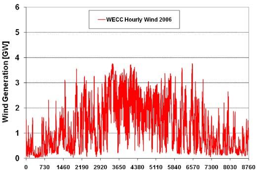
This page intentionally left blank

TABLE OF CONTENTS

1   BACKGROUND ..............................................................................................................       1

2   METHODOLOGY AND ASSUMPTION .......................................................................                              2

    2.1 Scope and Model Resolution ....................................................................................              2
    2.2 Analytical Process.....................................................................................................      3
    2.3 Data Collection and Preparation ...............................................................................              3
        2.3.1 Inventory of Existing and Proposed Power Plants.......................................                                 3
        2.3.2 Historical Load Data ....................................................................................              4
        2.3.3 Load Projections ..........................................................................................            4
        2.3.4 Fuel Price Projections ..................................................................................              4
        2.3.5 Expansion Candidate Technology Data .......................................................                            4
    2.4 Treatment of Renewable Generation (Hydro and Wind)..........................................                                 5
    2.5 Current Load and Load Forecast...............................................................................                6
    2.6 Load Adjustments .....................................................................................................       7
    2.7 Capacity Expansion Modeling..................................................................................                8
    2.8 Thermal Dispatch Modeling .....................................................................................             10

3   MODEL RESULTS ..........................................................................................................        12

    3.1 Base Year Model Calibration....................................................................................             12
    3.2 Baseline Results ........................................................................................................   13
        3.2.1 Load Projection ............................................................................................          13
        3.2.2 Capacity and Generation Projection.............................................................                       14
        3.2.3 CO2 Emissions Projection ............................................................................                 16
    3.3 Drought Scenario ......................................................................................................     17
        3.3.1 Major Scenario Assumptions .......................................................................                    17
        3.3.2 Impacts on Generation Mix and Generation Cost........................................                                 20
        3.3.3 Impacts on Electricity Prices........................................................................                 22
        3.3.4 Impacts on CO2 Emissions...........................................................................                   24

4   SUMMARY AND CONCLUSIONS ...............................................................................                         26

    4.1    Effect of Drought on Generation Mix.......................................................................               26
    4.2    Effect of Drought on Energy Prices and Water Supplies .........................................                          27
    4.3    Effect of Drought on CO2 Emissions........................................................................               27
    4.4    Effect of Drought on Use of Nuclear Power.............................................................                   28
    4.5    Areas for Future Study..............................................................................................     28

5   REFERENCES .................................................................................................................    30
LIST OF FIGURES
Figure 1: Map of WECC System .......................................................................................... 2
Figure 2: Example for Hydro Variability — Natural Flow for the Colorado River
at Lees Ferry .......................................................................................................... 2
Figure 3: WECC Hourly Wind Generation 2006.................................................................. 5
Figure 4: Hydropower Plant Operations ............................................................................... 5
Figure 5: Processing Hourly Loads....................................................................................... 6
Figure 6: RMPA and AZNM Monthly Energy Factors ........................................................ 7
Figure 7: RMPA and AZNM Monthly Peak Factors ............................................................ 7
Figure 8: Example for Load Adjustment............................................................................... 7
Figure 9: Example for Load Duration Curves....................................................................... 7
Figure 10: Annual Energy Outlook 2008 Electricity Market Model Supply Regions............ 8
Figure 11: Annual Peak Load Forecasts until 2020 ................................................................ 9
Figure 12: Creating a Thermal Unit Inventory........................................................................ 10
Figure 13: Example for Results of Maintenance Scheduling Routine .................................... 11
Figure 14: Model Calibration — Price Probability Distributions for January
through March 2006 .............................................................................................. 12
Figure 15: Model Calibration — Price Probability Distributions for April
to June 2006........................................................................................................... 13
Figure 16: Model Calibration — Price Probability Distributions for July
to September 2006 ................................................................................................. 13
Figure 17: Model Calibration — Price Probability Distributions for October
to December 2006.................................................................................................. 13
Figure 18: Baseline Projected Load, Existing System, and New Capacity Additions
until 2020 ............................................................................................................... 14Figure 19: Baseline Projected Total Installed Capacity until 2020......................................... 15
Figure 20: Baseline Projected Capacity Additions until 2020 ................................................ 15
Figure 21: Baseline Projected Total Installed Renewable Capacity until 2020 ...................... 16
Figure 22: Sample of Data Displayed on the U.S. Drought Monitor Web Site —
Western United States and Wyoming Drought Conditions as of
January 27, 2009.................................................................................................... 19
Figure 23: Electricity Generated by Fuel Type — Base and Drought Scenarios ................... 21
Figure 24: Production Cost and ENS Cost Differences between Base and
Drought Scenarios ................................................................................................. 22
Figure 25: Price Distribution for January and August 2010 ................................................... 23
Figure 26: Price Distribution for January and August 2015 ................................................... 24
Figure 27: Price Distribution for January and August 2020 ................................................... 24
LIST OF TABLES
Table 1: Generating Technologies Represented in the Electricity Market Module ............... 9
Table 2: 2006 Model Calibration for Generation Mix ........................................................... 12
Table 3: CO2 Emission Factor by Fuel Type ......................................................................... 17
Table 4: Amount of CO2 Emissions for Baseline Scenario ................................................... 17
Table 5: Quantity of Electricity Generated by Fuel Type — Base and
Drought Scenarios.................................................................................................... 20
Table 6: Average Monthly Price of Electricity — Base and Drought Scenarios................... 23
Table 7: Comparison of CO2 Emissions — Base and Drought Scenarios ............................. 24Prepared by:
Leslie Poch
Argonne National Laboratory
Guenter Conzelmann
Argonne National Laboratory
Tom Veselka
Argonne National Laboratory
Under Contract DE-AC02-06CH11357ACKNOWLEDGEMENTS The authors would like to thank members of the U.S. Department of Energy’s National Energy Technology Laboratory Existing Plants Research Program for entrusting Argonne National Laboratory with the responsibility for conducting this project in a thorough and unbiased manner.
1 BACKGROUND
This report was funded by the U.S. Department of Energy’s (DOE’s) National Energy
Technology Laboratory (NETL) Existing Plants Research Program. The energy-water research
component of this program is focused on water use at power plants. This study complements the
program’s overall research effort by evaluating the availability of water at power plants under
drought conditions.

During the summer and fall of 2007, a serious drought affected the southeastern United States.
River flows decreased, and water levels in lakes and other impoundments dropped. In a few
cases, water levels were so low that power production had to be stopped or reduced. It is likely
that, in coming years, competing water demands will increase. It is also possible that climatic
conditions will become warmer or at least more variable, thereby exacerbating future droughts.

This report attempts to identify the system-wide impacts on the power system that could arise
from various decreases in surface water levels. Our analysis is based on a separate report by
Kimmell and Veil (Kimmell and Veil 2009) that (1) evaluates the sources of cooling water used
by the U.S. steam-electric power plant fleet, (2) develops a database of cooling water intake
locations and depths for those plants that use surface water supplies, and (3) identifies steam-
electric power plants equipped with cooling water intakes that could not function if the water
levels were to drop below certain thresholds. The goal of the simulations is to quantify the
impacts of such water level decreases on the generation mix, future electricity prices, and carbon
dioxide (CO2) emissions that would occur if the utility and system operators were forced to take
any of those steam-electric plants out of service, or reduce their outputs, for extended periods of
time.

Our analysis focuses on the Western United States. We calibrate our power system dispatch
model to the year 2006 and then develop projections for future years. In this document, we report
results for 2010, 2015, and 2020.

                                                 1
2 METHODOLOGY AND ASSUMPTION
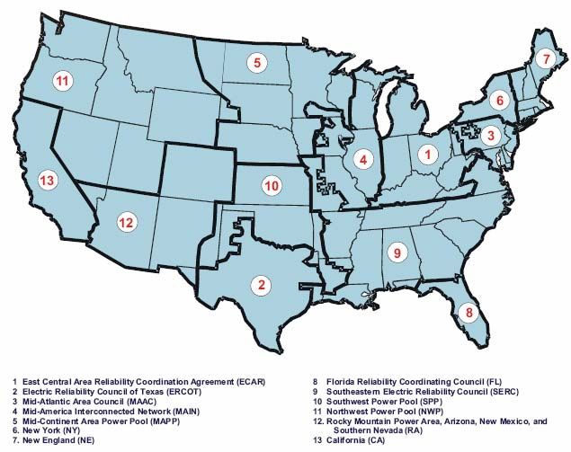
2.1 Scope and Model Resolution
We estimate future generation mix, future
electricity prices, and CO2 emissions by
simulating the operations of thermal and
renewable power plants in the Western
Electricity Coordinating Council (WECC)
system, particularly the portion of WECC that
is within the United States (Figure 1). The
WECC regions that we model include the
Northwest Power Pool (NWPP), Rocky
Mountain Power Area (RMPA), Arizona-New
Mexico-Southern Nevada Power Area
(AZNM), and California (CAL). We pay
special attention to interdependencies among
hydropower and thermal power plant
operations because hydropower plants may
provide up to 40% of the WECC load during Figure 1: Map of WECC system (Only
years when wet hydrological conditions occur. United States Considered for Modeling)
In some water basins, such as the Colorado
River System, annual hydropower generation can vary by more than a factor of five (Figure 2).
Hydrology conditions affect the dispatch of the thermal system, and therefore, water use by the
power sector.
Hydropower plant generation is 30 30
determined on an hourly time step. In Annual
10-Year Average
the current model implementation, we 25 25
Annual Flow [Million Acre-Feet]
Average
simulate hydropower as an aggregate
20 20
generation resource that serves both
base load and peaking duties. We 15 15
compile the information for the
aggregation from individual plant-level 10 10
data. The hourly dispatch of the
5 5
aggregate power plant is based on
(1) monthly generation control totals, 0 0
(2) the amount of water used for base 1905 1915 1925 1935 1945 1955 1965 1975 1985 1995 2005
Calendar Year
load duties, (3) estimated monthly
hydropower capability, and (4) a Figure 2: Example for Hydro Variability — Natural
Flow for the Colorado River at Lees Ferry
WECC-wide hourly load profile.
For electricity demand, we construct WECC-wide hourly electricity demand profiles for 2006 to
2020 from control area load profiles in combination with forecasts from the Annual Energy
Outlook 2008 (AEO 2008) published by DOE’s Energy Information Administration
(EIA 2008[a]).
2Thermal power plants are simulated at the unit level. We employ a probabilistic dispatch model
to simulate thermal power plant production to meet load that is not served by hydropower plants
and other renewable resources, such as wind power. We can run the thermal dispatch in two
modes: by either using monthly load duration curves (LDCs) or using hourly chronological
loads. In the first mode, we obtain monthly average capacity factors, generation levels, and
monthly price distributions. In the second mode, we obtain hourly price distributions. In both
modes, maintenance and random forced outages are accounted for at the unit level.
2.2 Analytical Process
We model the WECC–U.S. system dynamically for 2006–2020 using several modeling tools.
The methodology employs the following sequence of operations:
• Collect and process data and information;
• Determine hourly renewable generation, including dispatchable and non-dispatchable
aggregate hydropower and other non-dispatchable plants, such as wind;
• Determine current hourly electricity loads and forecast future load levels;
• Adjust loads for non-dispatchable renewable generation and hydropower plant
generation;
• Develop baseline capacity expansion plan until 2020;
• Run a probabilistic thermal dispatch model to estimate electricity generation by thermal
generation units from 2006 to 2020;
• Compute hourly prices chronologically and calculate monthly price distributions;
• Develop alternative drought scenarios;
• Run probabilistic dispatch model for the different scenarios to project hourly prices until
2020; and
• Compare and summarize results.
2.3 Data Collection and Preparation
The baseline analysis utilizes an extensive set of information. We compile the underlying data
from various sources; considerable effort is spent on data validation to ensure data consistency.
The following is a list of information sources used to compile the WECC-wide inventory of
existing and proposed power plants, hourly load profiles, load projections, fuel price projections,
and technology data.
2.3.1 Inventory of Existing and Proposed Power Plants
• Form EIA-860 (Annual Electric Generator Report) (EIA undated[a])
– Identifies the generator location
– Identifies the generator owner(s)
– Provides information on summer and winter generating capability
– Identifies the type of primary mover
– Identifies the fuel type(s) used by the generator
3• Form EIA-423 (Monthly Cost and Quality of Fuels Report) (EIA undated[a])
– Provides information on the price of the fuel(s) used by generator
– Provides information on the sources of the fuel(s) used by the generator
– Provides information on the quality of the fuel(s) used by the generator (e.g., sulfur
content, ash content, and higher heating value)
• Form EIA-906 (Power Plant Report) (EIA undated[a])
– Provides information on monthly fuel consumptions by generator
– Provides information on monthly generation levels by generator
• North American Electric Reliability Corporation (NERC) Generator Availability Data
Set (GADS) (NERC 2008)
– Provides scheduled maintenance outage rates by type of technology
– Provides random outages by type of technology
2.3.2 Historical Load Data
• Federal Energy Regulatory Commission (FERC) Form 714 (Annual Electric Balancing
Authority Area and Planning Area Report) (FERC 2009)
– Provides information on hourly load data by control area
2.3.3 Load Projections
• WECC near-term forecast (Summary of Estimated Loads and Resources) (WECC
2007[b]) and FERC Form 714 (FERC 2009)
– Provides information on monthly loads for two years into the future
– Provides information on seasonal loads for 3- to 10-year forecast period
• AEO 2008 (EIA 2008[a])
– Provides annual load projections until 2030
2.3.4 Fuel Price Projections
• AEO 2008 (EIA 2008[a]) projections
– Provides annual fuel price escalations by fuel type until 2030
2.3.5 Expansion Candidate Technology Data
• AEO 2008 (EIA 2008[a])
– Provides information on technical and economic performance parameters of
representative power generation technologies
42.4 Treatment of Renewable Generation (Hydro and Wind)
We first estimate non-dispatchable renewable power generation. From the detailed output tables
for the AEO 2008 reference case, we take the annual energy generation by renewable technology
until 2020 for the three regions used by
EIA to define WECC (Note: EIA
divides the U.S. into 13 regions and
three of those regions make up WECC,
while WECC subdivides itself into four
regions. EIA combines the WECC
regions of AZNM and RMPA into one
region, called RMPA-AZ. See Figure
10 in Section 2.7 for details).
Geothermal, municipal solid waste, and
wood and biomass combustion units are
included in the dispatch model. For
wind, we use a total of eight available
wind generation patterns for the Figure 3: WECC Hourly Wind Generation 2006
Western United States and assign them
as representative wind patterns to each
of the three EIA-defined regions that make up WECC to obtain hourly wind generation patterns
for each WECC region. We use a scaling routine to match the AEO 2008 regional wind energy
totals and sum across the regions to obtain a WECC-wide hourly wind generation trace until
2020 (Figure 3 shows Base Case WECC wind generation in 2006). This wind generation is then
subtracted from the total WECC load. We complete a similar load subtraction for non-
dispatchable hydropower (i.e., run-of-river power plants). Section 2.6 provides more details
about the load subtraction process.
To model the hourly generation pattern
from dispatchable hydropower plants 350 350
Total Capability: 150 MW
(plants with reservoirs or storage Peaking Capability: 100 MW
300 Minimum Release: 50 MW
Discretionary
Water Release 300
Generation: 1,910 MWh
capabilities), we use a peak shaving No Other Restrictions Peak Pattern (710 MWh)
approach. By using information from 250 Shaved 250
Generation [MWh]
Loads [MW]
Form EIA-906, we estimate monthly 200 200
hydropower generation patterns for
Mandatory Water
150 150
individual hydropower plants. Also, Release Pattern
(1200 MWh)
data from various sources are used to Remaining Loads
100 100
separate power plant capabilities
50 50
obtained from Form EIA-860 into base Minimum Release Rate
load and peaking duties. Total monthly 0 0
hydropower generation levels and plant 1 3 5 7 9 11 13 15 17 19 21 23
capabilities are then computed. Next, Figure 4: Hydropower Plant Operations
we simulate the hourly hydropower
dispatch by using a peak shaving
algorithm that minimizes the peak load that the thermal system must serve subject to monthly
hydropower capacity and energy constraints, spinning reserve duties, hourly ramping constraints,
and daily change limitations (Figure 4).
52.5 Current Load and Load Forecast
Figure 5 shows the process used to develop the hourly WECC load data for the analysis period
(2006–2020). First, we collect hourly historical load data for all control areas in the United States
Hourly FERC Form-714 Data
Control Area Loads Are by Control Area for 1993-2006
Separated into Power Pools
& Aggregated Hourly
NWPP (I) RMPA (II) AZNM (III) CAL (IV) NERC EIA
WECC EIA State
ES&D Coordinated
Annual
Hourly Loads Hourly Loads Hourly Loads Hourly Loads Data
Energy
Energy
Power Supply Database
1993-2006 1993-2006 1993-2006 1993-2006 Files Programs Outlook
Monthly Load
Control Totals
(Peak & Total
Representative Selected
Profile Load Shaping Energy)
Load Profile Monthly Peak and Total Loads
Algorithm by Power Pool for 2004-2025
Selection
NWPP (I) RMPA (II) AZNM (III) CAL (IV)
Hourly Loads Hourly Loads Hourly Loads Hourly Loads
2006-2020 2006-2020 2006-2020 2006-2020
WECC Hourly Loads
2006-2020
Figure 5: Processing Hourly Loads
that report to WECC. We perform consistency checks on the data, making adjustments when
errors are found and data are missing. Control area loads are then grouped and aggregated into
the four WECC regions: NWPP, RMPA, AZNM, and CAL. The areas only cover U.S. territory.
Next, we use a load-scaling algorithm to adjust aggregated hourly load profiles to exactly match
the monthly peak and total load values reported for each WECC region.
Figures 6 and 7 show relative monthly energy factors and monthly relative peak fractions based
on FERC Form 714 for two of the major areas (RMPA and AZNM) for a selection of historical
years. For each major area, we select from this data set, as the representative load profile, the
data set that has the lowest sum of squared differences relative to the average profile. This
representative profile is used as the basis for constructing hourly load projections for future years
through 2020. The load-scaling algorithm is applied to adjust the representative hourly load
profiles to match peak and total load targets that come from various statistics, including WECC’s
6coordinated power supply programs, EIA state energy databases, EIA’s AEO 2008, and the
Electricity Supply and Demand (ES&D) data from the NERC.
0.10 1.00
RMPA RMPA
Relative Monthly Peaks (Fraction)
Relative Monthly Energy (Fraction)
0.09 0.90
0.08 0.80
1.00
AZNM
Relative Monthly Peaks (Fraction)
0.11
AZNM 0.90
Relative Monthly Energy (Fraction) 0.10
0.07 0.70 0.80
0.09
Year-1 Year-1
0.08 0.70
Year-2 Year-1 Year-2 Year-1
0.06
0.07
Year-2 0.60 0.60
Year-2
Year-3
Year-3 0.06
Year-3
Year-4
Year-3 Year-4
0.50
Year-4 0.05 Year-4 Jan Feb Mar Apr May Jun Jul Aug Sep Oct Nov Dec
Jan Feb Mar Apr May Jun Jul Aug Sep Oct Nov Dec
0.05 0.50
Jan Feb Mar Apr May Jun Jul Aug Sep Oct Nov Dec Jan Feb Mar Apr May Jun Jul Aug Sep Oct Nov Dec
Figure 6: RMPA and AZNM Monthly Figure 7: RMPA and AZNM Monthly
Energy Factors Peak Factors
2.6 Load Adjustments
As discussed in Section 2.4, the original hourly total-WECC load data series are adjusted in two
ways:
1. For non-dispatchable resources (e.g., wind, run-of-river hydro) by using load subtraction.
2. For dispatchable hydropower using the peak shaving algorithm.
The remaining adjusted hourly loads are used to construct monthly LDCs that are served by the
thermal system and are input into the probabilistic thermal dispatch model for the simulations.
Figure 8 shows a 1-week example of how the load adjustments affect the total load served by the
thermal system. Figure 9 shows the monthly load duration curves.
180 160
Load Wind
160 LoadMinusWind Hydro
RemainingLoad
140
140
120
Power Level [GW]
120
100
Load [GW]
100
80
80
60 60
40 40 Load
Load Minus Wind
20 20
Remaining Load After Hydro
0 0
0 48 96 144 192 240 288 336 384 432 480 528 576 624 672 720
0 48 96 144 192 240 288 336 384 432 480 528 576 624 672 720
Figure 8: Example for Load Adjustment Figure 9: Example for Load Duration Curves
(WECC May 2020) (WECC May 2020)
72.7 Capacity Expansion Modeling
We develop the baseline capacity expansion scenario for the WECC system until 2020 by using
the EIA’s AEO 2008 as a starting point. EIA derives these projections by using the National
Energy Modeling System (NEMS) Electricity Market Module (EMM). On the basis of the fuel
prices and electricity demands provided by other modules of the NEMS, the EMM determines
the most economical way to supply electricity, subject to environmental and operational
constraints. A detailed description of the EMM is available in Electricity Market Module of the
National Energy Modeling System 2006 (EIA 2006).
The AEO 2008 contains projections of new capacity additions by technology for a total of
13 regions, shown in Figure 10.
Three of these regions represent a geographic area in the United States that is served by WECC:
• Region 11: Northwest Power Pool
• Region 12: Rocky Mountain Power Area, Arizona, New Mexico, and Southern Nevada
• Region 13: California
It should be noted that WECC defines four general load areas or regions within its service
territory:
1. Northwest Power Pool Area
2. Rocky Mountain Power Area
3. Arizona – New Mexico – Southern Nevada Power Area
4. California – Mexico Power Area
Figure 10: Annual Energy Outlook 2008 Electricity Market Model
Supply Regions (Source: EIA 2008[b])
8To maintain consistency with the
AEO 2008, our analysis uses a 80
representation of the WECC system 70
with three regions for the
60
development of the revised capacity
Peak Load (GW)
expansion plan. 50
40
Figure 11 shows the AEO 2008 peak
30
load forecasts for each of the WECC
regions. These load forecasts are 20 CA
RMPA/AZ
used to determine the needs for 10 NWPP
additional capacity until 2020.
0
2006 2008 2010 2012 2014 2016 2018 2020
The EMM analysis for the AEO
2008 considers a number of different Figure 11: Annual Peak Load Forecasts until 2020
candidate generating technologies.
As shown in Table 1, they include
both conventional and renewable technologies. The EMM analysis also allows for changing and
improving technical and economic parameters over time (i.e., learning parameters).
Table 1: Generating Technologies Represented in the Electricity Market Module (Source: EIA
2008[b])
Capacity Type
Existing coal steam plants
High sulfur pulverized coal with wet flue gas desulfurization
Advance coal - integrated coal gasification combine cycle
Advanced coal with carbon sequestration
Oil/gas steam - oil/gas steam turbine
Combined cycle - conventional gas/oil combined cycle combustion turbine
Advanced combined cycle - advanced gas/oil combined cycle combustion turbine
Advanced combined cycle with carbon sequestration
Combustion turbine - conventional combustion turbine
Advanced combustion turbine - steam injected gas turbine
Molten carbonate fuel cell
Conventional nuclear
Advanced nuclear - advanced light water reactor
Generic distributed generation - baseload
Generic distributed generation - peak
Conventional hydropower - hydraulic turbine
Pumped storage - hydraulic turbine reversible
Geothermal
Municipal solid waste
Biomass - integrated gasification combined cycle
Solar thermal - central receiver
Solar photovoltaic - single axis flat plate
Wind
9On the basis of the revised demand forecast for the WECC regions, we use a planning reserve
margin of 15% as a driver for new capacity additions until 2020. As stated in the WECC 2007
Power Supply Assessment (WECC 2007[a]), the capacity needs are determined at the level of
WECC regions, and each region needs to maintain a minimum planning reserve margin of 15%.
Because the reserve margin requirement is normally based on the net available capacity, while
the AEO 2008 lists only installed capacities, we have increased the requirement for the NWPP
region to 25% of installed capacity to account for the large amount of hydro capacity in this
region. The reserve margin requirements for the other two regions, RMPA/AZ and CAL, remain
at 15%. We then perform an expansion analysis for each region individually. Therefore, the total
capacity additions for the WECC system are obtained as the sum of new capacity additions in
each of the regions. The overall resulting reserve margin, based on the installed capacity, for the
WECC system as a whole, amounts to about 25% in 2012, gradually decreasing to about 21.4%
in 2020.
The technology mix of new generating capacity until 2020 is based on the AEO 2008 projections
for each WECC region. Compared with the AEO 2008 expansion plan, the 25% planning reserve
margin requirement does not produce any changes in the capacity needs for the NWPP region,
while the 15% reserve margin requirement requires some new generating capacity to be added to
the system in addition to that already projected by the AEO 2008. For the RMPA/AZ region, this
results in only slightly increased capacity needs beginning in 2019 and amounting to a
cumulative total of 1,160 MW by 2020. For the CAL region, the 15% reserve margin
requirement results in additional capacity needs beginning in 2012 and amounting to a
cumulative total of 9,850 MW by 2020. Again, it is assumed that the technology mix for this
additional capacity corresponds to that of the AEO 2008.
2.8 Thermal Dispatch Modeling
The first step in the dispatch
modeling is to create a validated
unit inventory for the entire Thermal Unit Outages
Inventory Rates
WECC system. As shown in EIA-860 GADS
Figure 12, we use Form EIA-
860 as a starting point, Fuel Prices Heat Rates Final Variable O&M
EIA AEO
Form EIA-423 to add fuel data EIA-423 EIA-906 Inventory
to the inventory, Form EIA-906
to obtain estimates for heat Water Use
& FGD
rates, the GADS database on EIA 767
outage information, and the
AEO 2008 tables for variable Figure 12: Creating a Thermal Unit Inventory
operation and maintenance
(O&M) costs.
With the complete unit inventory, we run a unit-level hourly thermal probabilistic dispatch
model that accounts for forced outages, as well as scheduled maintenance. We estimate future
maintenance schedules by using a routine that maximizes the minimum reserve margin.
Figure 13 shows sample results for the maintenance scheduler in combination with a forced
1055 55
P lan n ed & M ain ten an ce O u tag es L o ad O n -L in e C ap acity
50 50
45 45
40 40
Capacity/Load [GW]
35 35
30 30
25 25
20 20
15 15
10 10
5 5
0 0
Jan Feb M ar A p r M ay Jun Ju l A u g S ep O ct N ov D ec
Figure 13: Example for Results of Maintenance Scheduling Routine
outage scenario. The dispatch model utilizes a convolution process in which the loads that a unit
serves include (1) the original LDC and (2) loads that could not be served by units loaded before
it because of forced outages.
From the dispatch routine, we obtain unit-level generation levels, chronological prices, price
distributions, and CO2 emissions and summarize them for each simulation month. Hydropower
plants in this analysis are modeled as an aggregate generation resource that serves base load and
peaking duties. The hourly dispatch of the aggregate power plant is based on monthly generation
control totals, the amount of water used for base load duties, estimated monthly hydropower
capability, and a WECC-wide hourly load profile.
113 MODEL RESULTS
3.1 Base Year Model Calibration
We use information for 2006 to calibrate the model to actual observed WECC market data. Table
2 provides a comparison of model results with actual annual generation and fuel consumption
data by fuel type.
Table 2: 2006 Model Calibration for Generation Mix
Technology Model Generation Mix (%) Actual Generation Mix (%)
Coal 31.5 31.2
Gas 26.2 25.6
Nuclear 10.4 9.4
Hydro 28.1 28.8
Wind 1.6 1.4
Others 2.2 3.6
Total 100 100
Note: Actual generation mix is calculated based on AEO 2008.
In addition to generation and fuel consumption levels, we test and calibrate the model with
regard to historical prices, collecting prices from the following hubs in WECC for several
historical years: Palo Verde, Pinnacle Peak, 4Corners, Mona, Mead, COB, NP15, SP15,
MidColumbia, NOB, and WestWing. Prices are available in off-peak and on-peak blocks. We
adjust the data set to account for the fact that off-peak prices are for 8-hour blocks, on-peak
prices are for 16-hour blocks, and prices on Sundays are for 24-hour blocks. WECC system
holidays are considered off-peak. From the hub prices, we calculate an average WECC system
price that we compare with our modeled unconstrained system marginal price. Figures 14
through 17 show the results of the calibration process. The red bars show the price probability
distributions from our model runs for each month in 2006. The blue lines show the monthly
probability distribution of the estimated average WECC system price derived from daily hub
prices for 2006.
0.40 0.40 0.40
January 2006 February 2006 March 2006
0.35 0.35 0.35
0.30 0.30 0.30
0.25 Model Actual 0.25 Model Actual 0.25 Model Actual
0.20 0.20 0.20
0.15 0.15 0.15
0.10 0.10 0.10
0.05 0.05 0.05
0.00 0.00 0.00
0 50 100 150 200 250 300 350 400 0 50 100 150 200 250 300 350 400 0 50 100 150 200 250 300 350 400
Figure 14: Model Calibration — Price Probability Distributions for January through March 2006
120.40 0.40 0.40
April 2006 May 2006 June 2006
0.35 0.35 0.35
0.30 0.30 0.30
0.25 Model Actual 0.25 Model Actual 0.25 Model Actual
0.20 0.20 0.20
0.15 0.15 0.15
0.10 0.10 0.10
0.05 0.05 0.05
0.00 0.00 0.00
0 50 100 150 200 250 300 350 400 0 50 100 150 200 250 300 350 400 0 50 100 150 200 250 300 350 400
Figure 15: Model Calibration — Price Probability Distributions for April to June 2006
0.40 0.40 0.40
July 2006 August 2006 September 2006
0.35 0.35 0.35
0.30 0.30 0.30
0.25 Model Actual 0.25 Model Actual 0.25 Model Actual
0.20 0.20 0.20
0.15 0.15 0.15
0.10 0.10 0.10
0.05 0.05 0.05
0.00 0.00 0.00
0 50 100 150 200 250 300 350 400 0 50 100 150 200 250 300 350 400 0 50 100 150 200 250 300 350 400
Figure 16: Model Calibration — Price Probability Distributions for July to September 2006
0.40 0.40 0.40
October 2006 November 2006 December 2006
0.35 0.35 0.35
0.30 0.30 0.30
0.25 Model Actual 0.25 Model Actual 0.25 Model Actual
0.20 0.20 0.20
0.15 0.15 0.15
0.10 0.10 0.10
0.05 0.05 0.05
0.00 0.00 0.00
0 50 100 150 200 250 300 350 400 0 50 100 150 200 250 300 350 400 0 50 100 150 200 250 300 350 400
Figure 17: Model Calibration — Price Probability Distributions for October to December 2006
3.2 Baseline Results
3.2.1 Load Projection
We project that electricity demand in the WECC–U.S. system will increase from about 700 TWh
in 2006 to over 930 TWh in 2020 with a corresponding growth in peak load — from over
135 GW to almost 170 GW over the same period. With this growth in load, the expected
retirement of approximately 7.8 GW of existing generating units, and the need to maintain an
adequate planning reserve margin, we foresee a need to bring online new capacity on the order of
1350 GW by 2020. Figure 18 shows the capacity-load balance for the WECC system, illustrating
the development of existing and new generating capacity versus the peak load until 2020.
300
W ECC - Capacity-Load Balance
250
Capacity/Load (GW)
200
150
100
New Capacity Ad dition s
50
Existin g System Capacity
Peak L oad
0
2006 2008 2010 2012 2014 2016 2018 2020
Figure 18: Baseline Projected Load, Existing System, and New Capacity Additions until 2020
3.2.2 Capacity and Generation Projection
Figure 19 illustrates the development of generating capacity by technology type over the
projection period. Total installed capacity grows from 177 GW in 2006 to 212 GW in 2020. Fuel
oil capacity drops from 20 to 14.6 GW. Existing nuclear units will be allowed to retire according
to schedule with no new nuclear capacity assumed to come online during the study period in the
WECC system. Major growth is projected for coal and renewables, with increases from 32 to 59
GW and 59 to 66 GW, respectively, with an additional 350 MW of small distributed generation
capacity.
Figure 20 shows the technology mix of the new capacity additions. By 2020, a total of 50 GW of
new capacity is projected to come on line. Coal takes the largest share with 27 GW (55% of total
additions), followed by 14 GW of gas-fired units (29%), and 8 GW of renewables and small
distributed generators (16%). We also assume that new coal plants will be equipped with a
cooling system that will be much less vulnerable to drought conditions, such as dry cooling
(which requires little or no water).
14300
WECC - Total Capacity by Technology Type
250
Coal Nuclear Natural Gas
Fuel Oil Pumped Storage/Other Distributed Generation
Generating Capacity (GW)
Renewable Sources
200
150
100
50
0
2006 2008 2010 2012 2014 2016 2018 2020
Figure 19: Baseline Projected Total Installed Capacity until 2020
1550
W E C C - Ne w Ca p ac ity Ad d ition s
45
40
Generating Capacity (GW)
35 Ren ew a ble So u rces
Distribu ted G en eration
P um pe d St orag e/O th er
30 F u el O il
Nat ural Ga s
25 Nu clear
Co al
20
15
10
5
0
2006 2008 2010 2012 2014 2016 2018 202 0
Figure 20: Baseline Projected Capacity Additions until 2020
Figure 21 provides a breakdown of renewable capacity for the WECC system until 2020.
Conventional hydro capacity essentially stays flat at around 52 GW. Geothermal and wind
increase from 2.4 to 3.1 GW and from 5.1 to 8.1 GW, respectively. Most of the renewable
capacity additions come from hydropower (2 GW), wind (3 GW), and geothermal (0.7 GW),
with the balance coming from smaller amounts of solar thermal and solar photovoltaic (PV),
municipal solid waste, and wood/biomass.
1680
WECC - Renewable Generating Capacity
70
60
50
Capacity (GW)
40
Wind
30 Solar Photovoltaic
Solar Thermal
Wood and Other Biomass
20 Municipal Solid Waste
Geothermal
Conventional Hydropower
10
0
2006 2008 2010 2012 2014 2016 2018 2020
Figure 21: Baseline Projected Total Installed Renewable Capacity until 2020
3.2.3 CO2 Emissions Projection
Carbon dioxide emissions result from the combustion of fuels containing carbon. In this study,
the carbon-based fuels are coal, natural gas, fuel oil, and biomass. Because CO2 emissions from
biomass are highly dependent upon its composition, and because biomass makes up only about
1% of the generating capacity in the western United States, emissions from biomass power plants
are not addressed in this study.
For the remaining thermal plants, CO2 emissions vary by plant and depend on the fuel type, the
efficiency of the power plant (or heat rate [measured in Btu/kWh]), and the amount of electricity
the plant produces.
Emissions of CO2 are calculated by using an emission factor. Emission factors have been
developed for all types of carbon-based fuels; they measure the amount of CO2 released (in lb)
per unit of heat (Btu) generated during combustion. Emission factors for this study were obtained
from the EIA Web site and are listed in Table 3. The value for coal is the average of the emission
factor for bituminous and sub-bituminous coals, which are the two types of coal used in power
plants in the western United States.
Table 3: CO2 Emission Factor by Fuel Type
17CO2 Emission
Fuel Type Factor
(lb/million Btu)
Coal 209.0
Natural Gas 116.4
Heavy Fuel Oil 173.7
Light Fuel Oil 161.3
Source: EIA undated[b].
One of the results of the baseline thermal dispatch model run is the amount of electricity each
plant in the unit inventory produces each month of the year. The unit database contains the
efficiency or heat rate of each plant. Multiplying each plant’s emission factor by the heat rate and
the amount of electricity it generates in a year yields the amount of CO2 the plant produces.
Summing the CO2 emissions from all the plants in the inventory yields the total amount of CO2
produced by the electric power system. Table 4 lists the CO2 emissions produced in each year of
the study period.
Table 4: Amount of CO2 Emissions
for Baseline Scenario
CO2 Emissions
Year
(million short tons)
2010 408.4
2015 480.5
2020 548.1
3.3 Drought Scenario
This section discusses the major assumptions behind the drought scenario and compares the
results of the thermal dispatch model runs for the baseline and drought scenarios with respect to
generation mix, electricity prices, and CO2 emissions.
3.3.1 Major Scenario Assumptions
A drought would adversely impact not only thermal power plants that use fresh surface water for
cooling, but also hydroelectric power plants. Hydropower production affects the load that must
be served by the thermal systems, including power plants that do not rely on surface water. As
hydropower generation is reduced as a result of drought conditions, the thermal system must
operate at a higher level to compensate for lower hydropower production levels. The WECC
electric grid relies very heavily on hydroelectric power. Approximately 28% of the electric
power capacity is supplied by hydroelectric power plants; this percentage increases to as much as
40% in a wet hydrologic year. Therefore, to accurately simulate the effects of drought on power
system operations in the WECC, we must determine the impacts of a drought on hydroelectric
power generation.
18In order to determine how much the amount of electricity generated by hydroelectric power
plants would be reduced as the result of a severe drought, we reviewed data on hydroelectric
output from 1980 and 2005. We selected 1980 as the first year of the review period because the
vast majority of current WECC hydropower capacity was on line in that year, and only a very
small amount of that capacity had been retired during that time period. After reviewing this
hydroelectric power generation data, we selected the year with the lowest hydroelectric power
production to be representative of a year in which hydropower was most affected by severe
drought conditions. We assumed that the monthly amount of generation and the capacity pattern
for this historic low-hydropower year would represent the operation of hydroelectric power
plants in each analysis year of the drought scenario.
After determining the hydroelectric generation pattern for the drought scenario, we calculate the
load pattern to be supplied by the dispatchable thermal power plants using the method described
in Section 2.4 (i.e., the nondispatchable or run-of-river hydroelectric generation value is
subtracted from the hourly loads remaining after wind generation is subtracted from the original
WECC loads). The peak shaving algorithm is then used to model the hourly generation pattern
from dispatchable hydroelectric power plants and, ultimately, to calculate the hourly loads to be
supplied by thermal power plants.
The inventory of thermal power plants in the WECC system that may be adversely impacted by a
drought is based on a task performed by another Argonne team and described in a separate report
(Kimmell and Veil 2009). Kimmel and Veil developed a database identifying fossil and nuclear
power plants equipped with cooling systems that use fresh surface water. Data included plant
name, location, plant code, owner, fuel type, nameplate capacity, source of cooling water, depth
of cooling water intakes, and other characteristics.
As stated in that report, drought conditions can be highly variable across the United States; they
can affect large areas of the country for a long period or small areas for a short period. Because
of this variability, it is highly unlikely that all of the thermal power plants using surface water for
cooling would have to shut down or curtail operations in an area as large as the western United
States during a drought, regardless of the depth of their water intakes. Therefore, simultaneous
shutdown of all power plants in the WECC system as the result of a drought would probably be
an unrealistic scenario.
Consequently, we employ an alternative approach, using the information available on the U.S.
Drought Monitor (University of Nebraska Lincoln 2009), a Web site funded by several Federal
agencies and operated by the University of Nebraska Lincoln. Researchers compile and archive
drought conditions on a weekly basis, from 2000 to the present, and post them on the Web site.
Drought conditions are shown graphically by state and also by county within each state.
19For this study, we chose drought conditions for the week of January 27, 2009, to develop a
plausible drought scenario and to illustrate Argonne’s electric power system simulation
methodology. Figure 22 shows how data are displayed on the Web site on a regional and state
basis.
Figure 22: Sample of Data Displayed on the U.S. Drought Monitor Web Site — Western
United States and Wyoming Drought Conditions as of January 27, 2009
(University of Nebraska Lincoln 2009)
To identify the plants that could be affected by the drought conditions during the chosen week,
we compare the locations of the power plants in the WECC system with the maps on the
U.S. Drought Monitor (University of Nebraska Lincoln 2009). We obtain the locations, in
latitude and longitude coordinates, for each plant from the database of power plants developed
by the companion Argonne study (Kimmell and Veil 2009). A geographical information system
(GIS) program is used to plot the locations of the WECC power plants in the database; each
location is visually compared with the state maps in the U.S. Drought Monitor. If a power plant
was located in a part of the state that was designated as undergoing a moderate or more severe
drought, it was chosen for shutdown or curtailment in each year of the study period.
20By using this methodology, we identified a total of five plant sites in four states that would be
shut down or for which operations would be curtailed. The total capacity of these plants is 3,284
MW; 2,820 MW (or 86%) of this total is supplied by coal-fired power plants. Because
combined-cycle plants are very prevalent in the WECC system, their operation was handled in a
special manner in this analysis. Combined-cycle plants consist of a gas turbine and a steam
turbine that can be operated independently of one another, depending upon the configuration;
typically, the gas turbine can operate independently of the steam turbine. The steam turbine is the
only component that requires water for cooling. Therefore, in cases in which combined cycle
plants were identified as possible candidates for shutdown during a drought, only the steam
turbine portion of a combined-cycle unit was shut down.
3.3.2 Impacts on Generation Mix and Generation Cost
By using the technique described in Section 3.3.1, we determined the amount and generating
pattern of hydroelectric power plants during a drought. Our analysis revealed that, in a severe
drought year, the electrical generation from hydroelectric can drop by almost 30%. These data
were input into the thermal dispatch model, and simulations were run for the two scenarios for
2010, 2015, and 2020. Table 5 and Figure 23 show model results for the amounts of electricity
produced by fuel type. The amount of energy not served (ENS) is also shown. Energy not served
is the amount of energy demanded by customers that the system’s energy sources are unable to
provide. This energy must be supplied by a source outside of the system or system operators
must take steps to reduce load.
Table 5: Quantity of Electricity Generated by Fuel Type — Base and Drought Scenarios
Base Scenario Energy (TWh) Drought Scenario Energy (TWh)
Fuel 2010 2015 2020 2010 2015 2020
Nuclear 74.7 74.7 74.7 74.7 74.7 74.7
Coal 257.1 314.2 417.5 236.5 293.6 401.9
Natural Gas 244.9 252.1 161.1 320.1 326.1 231.0
Fuel Oil/Other 0.90 0.90 0.78 0.91 0.93 0.86
Renewable 36.8 44.4 47.1 36.8 44.4 47.1
Hydro 186.4 185.2 185.8 131.6 131.6 131.3
ENS 0.036 0.124 0.030 0.161 0.259 0.065
Total 800.8 871.6 886.9 800.8 871.6 886.9
In the drought scenario, electricity generated from coal dropped by 20.6 TWh (about 8%
compared with the baseline) in 2010, by 20.6 TWh (6.6%) in 2015, and by 15.6 TWh (3.7%) in
2020. The 30% drop in generation from hydroelectric power during a drought resulted in about
54 TWh less hydroelectric energy generated in the drought scenario. A significant increase in
generation from plants using natural gas compensated for the shortfall in generation from coal
and hydropower. Electricity production from natural gas rose by 75.3 TWh (30.8% compared
with the baseline) in 2010, 74 TWh (29.3%) in 2015, and 70 TWh (43.5%) in 2020. Generation
from other fuel sources, such as fuel oil and renewables, rose only slightly — no more than
0.1 TWh in any simulated year. Natural gas plants made up for almost the entire amount of
electricity not generated by coal and hydropower.
21Generation by Fuel Type and Scenario
1,000
Generation (TWh)
800
ENS
Hydro
600 Renewable
Fuel Oil/Oth
Nat. Gas
400
Coal
Nuclear
200
0
Base / Drought Base / Drought Base / Drought
2010 2015 2020
Year
Figure 23: Electricity Generated by Fuel Type — Base and Drought Scenarios (Note: The
quantity of ENS and Fuel Oil/Other cannot be seen on this plot because of its small amount
compared with the amount from other sources.)
The reason that natural gas plants were able to generate most of the electricity lost as a result of
coal plant shutdown and the reduction in hydropower can be seen by examining their capacity
factors from the base scenario model runs. The capacity factors of natural gas plants in 2010,
2015, and 2020 were 37.4%, 36.7%, and 23.1%, respectively. Because their capacity was not
fully utilized, they were able to pick up the slack in the drought scenario. By 2020 though, coal’s
contribution starts rising, while the contribution of natural gas begins to fall. This is because coal
plants with cooling technologies less vulnerable to drought are being installed in greater numbers
and, by 2020, begin to displace generation from natural gas plants which, in 2010 and 2015,
picked up the slack for generation from coal plants lost to drought conditions.
Nuclear power plants were unable to supply additional generation capacity in the drought
scenario for two reasons: (1) no new nuclear plant came online during the study period, and
(2) nuclear provides base load electricity and already generates up to its maximum potential even
in the base case. There was no excess nuclear capacity to generate more electricity. In the WECC
system, it is also fortunate that cooling water for nuclear power plants comes predominately from
sources other than fresh surface water; otherwise, they may have been subject to the drought
shutdown.
The amount of ENS increased significantly in the drought scenario, rising by more than 3.5 times
in 2010 and more than doubling in 2015 and 2020. Furthermore, if ENS occurs, there is more
than a 99.9% chance that it would occur in either July or August because demand for electricity
in the WECC peaks during the summer months.
22Because of the sharp increase in electricity produced by natural gas plants in the drought
scenario, the cost to produce electricity compared with the cost in the baseline scenario increased
sharply as well. This is because operating costs of natural gas plants can be more than 3 times
that of coal plants. Total electricity production costs in the baseline scenario were $17.9 billion
in 2010, $17.8 billion in 2015, and $15.2 billion in 2020. Total ENS costs in the baseline
scenario were $33.9 million in 2010, $124 million in 2015, and $30.9 million in 2020. Figure 24
shows the differences in production costs and ENS costs between both scenarios. Production
costs rose by $4.5 billion (25.2%) in 2010, $3.9 billion (21.9%) in 2015, and $3.5 billion (22.9%)
in 2020. Costs of ENS rose by $126 million in 2010, $135 million in 2015, and $33.4 million in
2020, assuming that ENS is valued at about $1000/MWh. This is considered a conservative
value; surveys have indicated that the cost of ENS can frequently exceed $2,000/MWh (Cramton
and Lien 2000).
Production costs and ENS costs decrease over time because new coal plants with cooling
technologies less vulnerable to drought begin displacing generation from natural gas plants,
whose generation increased in 2010 and 2015 to make up for generation lost from existing coal
plants as a result of drought conditions. The new coal plants are more efficient and much less
expensive to operate.
5.00
Production Cost Difference
Cost (billion$)
4.00 ENS Cost Difference
3.00
2.00
1.00
0.00
2010 2015 2020
Year
Figure 24: Production Cost and ENS Cost Differences between Base and Drought Scenarios
3.3.3 Impacts on Electricity Prices
The thermal dispatch model generates a variety of price outputs, including monthly price
distributions and hourly chronological prices with associated uncertainty ranges for user-
specified percentiles. Table 6 lists average monthly system-wide electricity prices, calculated on
the basis of monthly price distributions obtained from the model.
23Table 6: Average Monthly Price of Electricity — Base and Drought Scenarios
Average Price of Electricity ($/MWh) Price Difference
Base Scenario Drought Scenario (%)
Month 2010 2015 2020 2010 2015 2020 2010 2015 2020
Jan 61.01 54.04 51.76 65.97 58.32 56.79 8.1 7.9 9.7
Feb 60.21 53.30 50.67 67.21 59.40 54.29 11.6 11.5 7.2
Mar 55.58 49.14 46.02 60.84 53.38 50.69 9.5 8.6 10.1
Apr 54.95 48.47 43.61 61.08 53.45 50.27 11.1 10.3 15.3
May 54.69 46.88 40.57 62.23 53.06 48.29 13.8 13.2 19.0
Jun 55.35 48.71 40.04 61.80 54.96 47.48 11.7 12.8 18.6
Jul 69.14 68.07 54.17 91.67 89.16 67.24 32.6 31.0 24.1
Aug 78.48 87.87 61.75 105.70 109.75 71.27 34.7 24.9 15.4
Sep 59.97 52.85 44.95 64.05 56.73 50.17 6.8 7.3 11.6
Oct 63.20 55.75 43.04 65.47 57.86 47.24 3.6 3.8 9.8
Nov 62.97 55.36 52.13 65.89 58.18 56.36 4.6 5.1 8.1
Dec 59.44 52.70 50.89 66.72 58.71 55.30 12.2 11.4 8.7
The difference in the average price between the two scenarios is highest in the summer months
(July and August), when demand in the WECC regions peaks. In 2010 and 2015, the average
price for the drought scenario was 25–35% higher in those months. The difference in average
prices drops considerably with time. In 2010, the average drought price in August was 35%
higher than the base scenario price, but by 2020, the price was only 15% higher.
The distribution of prices is shown in Figures 25, 26, and 27 for January, a typical winter month,
and August, the peak summer month. The price distribution is much larger for August compared
with January for all years. In fact 5–10% of the time, prices exceed $150/MWh in August 2010
and 2015 in the drought scenario. That probability drops to about 2% in August 2020. Also, as
the study progresses, the price distribution for both scenarios shifts toward lower prices.
0.6 0.6
0.5
January 2010 0.5
August 2010
Price Probability
Price Probability
0.4 0.4
0.3 Base 0.3
Base
Drought
Drought
0.2 0.2
0.1 0.1
0.0 0.0
100 - 100
15 1 5
20 20
- 25
35 35
40 40
45 45
50 50
60 6 0
65 65
- 70
80 8 0
85 85
- 90
20 20
25 25
- 30
- 35
45 4 5
50 5 0
55 55
60 60
70 7 0
75 7 5
- 80
85 85
95 - 95
10 1 0
50
10 10
50
105 - 105
110 - 110
115 - 115
12 0 - 12 0
125 - 125
130 - 130
135 - 135
140 - 140
14 5 - 14 5
>1 0
105 - 105
110 - 110
115 - 115
12 0 - 12 0
125 - 125
130 - 130
135 - 135
14 0 - 14 0
145 - 145
>1 0
100 - 100
30 30
55 55
75 75
95 - 95
15 - 15
40 - 40
65 65
90 - 90
5- 5
5- 5
- 15
- 15
0-
0-
-
-
-
-
-
-
-
-
-
-
-
-
-
-
-
-
-
-
-
-
-
-
-
25
70
90
30
35
80
Pr ice ($/MWh) Price ($/MWh)
Figure 25: Price Distribution for January and August 2010
24You can also read