An insurable risk analysis for construction projects and industry using - sersc

International Journal of Advanced Science and Technology
 Vol. 29, No. 7, (2020), pp. 13507 - 13525

 An insurable risk analysis for construction projects and industry using
 SPI: Gauteng Province, South Africa

 Authors: Bernard Moeketsi Hlalele;
 hlalele.moeketsi@gmail.com
 Central University of Technology, Free State, Department of Business Support Studies
 Bloemfontein, 9301, Faculty of Management Sciences
 Abstract

The South African construction sector accounts for 11% of the total employment, thus contributing
approximately 4% of the country’s Gross Domestic Product (GDP). However, severe unpredictable
weather patterns can send this sector’s costs skyrocketing and revenue spiralling. Construction
industry is said to be a good indicator for economic growth. The aim of this current study was to
assess rainfall variability in the current rapidly changing climate regime, to set an avenue for
businesses’ opportunities and risk reduction adaptation measures in order to keep this industry in the
market. Annual rainfall data sets from eight weather stations were collected from an online source for
analysis. A non-parametric test, Pettitt’s homogeneity and Shapiro-Wilk tests for data stationarity and
normality respectively were deployed. A further Mann Kendall’s trend test was used to detect if any
monotonic trend patterns were existent in the data sets. The probability of non-exceedance and return
level periods were computed for each station. ANOVA test revealed all stations statistically different
in rainfall patterns. The major results for this study, was that (i) no statistically significant decreasing
patterns were observed over all candidate stations (ii), for every 2 to 5-year return periods, all
stations are to experience near-normal drought conditions as computed from Standardised
Precipitation Index (SPI). Given the frequent and intense drought episodes in South Africa and other
parts of the world, Gauteng province remains a relatively conducive environment for construction
business projects.

Keywords: drought, project risk, hazard, construction business, SPI, insurable risk

Introduction

Drought is described as a period in time whereby conditions are drier than normal and there is less
rainfall than usual for a long period of time; this could be for several weeks, months and years which
lead to water-related problems (Praveen, Ramachandran, Jaganathan, Krishnaveni, & Palanivelu,
2016). Needless to say, there is no specific definition of drought; however, it can be classified into
four main types. In this study, drought is described as a severe condition which is characterized by a
dry spell which has negative impacts on the economy, society and environment. The four main types
of drought are: meteorological drought, hydrological drought, agricultural drought and socio-
economic drought. (i) Meteorological drought is referred to as the degree of dryness compared to
normal conditions and this is uneven over time and particular regions (Olivares Campos, 2016), (ii)
ISSN: 2005-4238 IJAST
Copyright ⓒ 2020 SERSC
 13507

International Journal of Advanced Science and Technology
 Vol. 29, No. 7, (2020), pp. 13507 - 13525

hydrological drought refers to insufficient rainfall which leads to serious reduction in run-off
streamflow, inflow into storage reservoirs and revitalizing of groundwater (Orlando Olivares &
Zingaretti, 2018), (iii) Agricultural drought refers to a deficit of soil moisture to sustain plants and
livestock thereby causing redundant growth and reduced produce (Tefera, Ayoade, & Bello, 2019)
and Socio-economic drought refers to a period in which human activities are poorly affected by
reduction in water availability and precipitation. (Praveen et al., 2016). Much as all these types of
drought have a connection, one leads to another and sometimes overlaps; so, agricultural drought is
regarded as of prime importance and a roadmap in this study. The diagram below illustrates the
interrelationship of the types of drought.

Figure 1: Sequence of drought types’ occurrence and their impacts
Source: National Drought Mitigation Centre, 2012.

Key driving forces behind drought events

El Niño-Southern Oscillations

Of all the hemispheres (north, south of the equator; east and west of the Greenwich Meridian), Africa
is the only continent that lies within them all and is affected by numerous climatic conditions.
(Roman-Cuesta, 2007). Consequently, this continent receives conventional rainfall. (Choi, An Prof.,
Yeh, & Yu, 2013). This also gives rise to different climatic conditions such as El Nino. El Nino is a

ISSN: 2005-4238 IJAST
Copyright ⓒ 2020 SERSC
 13508

International Journal of Advanced Science and Technology
 Vol. 29, No. 7, (2020), pp. 13507 - 13525

recurring climate pattern which is caused by changes in temperatures of water by warming the eastern
Pacific, and therefore affecting the global climate. (Ali & Ali, 2011). This natural occurrence is
responsible for exacerbating drought events in the southern hemisphere. (Ali & Ali, 2011). In
accordance to Keil, Zeller, Wida, Sanim, & Birner (2008), drought is a resultant of the shifting,
changing weather patterns. On the other hand, it is also a belief that droughts chiefly transpire because
of natural occurrences due to the earth and atmospheric systems. However, Granzow-de la Cerda,
Lloret, Ruiz & Vandermeer (2012) are of the belief that no one knows for sure why droughts occur,
despite the fact that many scientists believe that there is a relationship between drought occurrence
and El Nino events. Enhanced understanding of the relationships between droughts and repeated
changes in high and low pressures from one side of the Pacific to the other linked with La Nina allow
scientists to formulate improved predictions of this cataclysmic drought hazard. (Ryu, Svoboda,
Lenters, Tadesse, Knutson 2010). Both El Nino and La Nina form the El Nino-Southern Oscillation
(ENSO) cycle. ENSO is a recurring climate pattern whereby temperature fluctuate between the ocean
and atmosphere in the east-central Equatorial Pacific, approximately between the International Date
Line and 120 degrees West (Olivares Campos, 2016). Nevertheless, these two events happen every 2-
7 years with El Nino events occurring more often than those of La Nina (Tefera et al., 2019). There
has been a rising trend in global weather disasters since 1980, and with extreme climatic events such
as droughts. (Orlando Olivares & Zingaretti, 2018). Comprehending phenomena such as ENSO is
pivotal because of the possibility that it could cause an enormous loss of property, destruction to the
environment and the loss of human life. Forecasts by ENSO, tracking and monitoring play a
significant role to insurers, government authorities and other pertinent stakeholders for drought
management for proactive planning against unfavourable impacts such as acute climatic changes like
drought events. (Praveen et al., 2016)

Solar activity (Sunspots number)

Drought could also be associated with sunspots which commonly last for a period of approximately
11 years. (Minckley, Roulston, & Williams, 2013). Sunspots are described as cool surface areas on
the sun that are visible in pairs and are darker in comparison with other parts of the sun. These spots
have a strong magnetic field and rotate like a giant hurricane. (Mèthy, Damesin, & Rambal, 1996).
These authors also affirm that several authors have acknowledged that sunspots have impacts on
temperature, precipitation, length of growing seasons, air circulation, atmospheric pressure, high
altitude, wind speed and other natural phenomena around the world. Moreover, Xiao & Zhuang
(2007) construct solar activity as a main cause of cyclic deviations of the global climate through
triggering of the evaporation processes. Scientists have also shown that sunspot numbers and drought
events are correlated. For instance, during solar activity- drought events take place at solar maximum
(Solheim, Stordahl, & Humlum, 2011). This occurrence is related t climatic conditions where

ISSN: 2005-4238 IJAST
Copyright ⓒ 2020 SERSC
 13509

International Journal of Advanced Science and Technology
 Vol. 29, No. 7, (2020), pp. 13507 - 13525

temperatures become high during solar maximum (Minnis, 1958). Solar energy is the principal energy
source as well as control on evaporation; therefore distributions of insulation and evaporation are
strongly linked. (Siingh et al., 2011). The energy from the sun is the central source of energy present
for heating the surface of the planet earth. This energy supplied by the sun is an outcome of its
activity and it differs with time. The major cycle of the sun is eleven years. The major cause of
drought events is believed to be the solar activity (Ghormar, 2014). The coefficient of correlation
between insolation and evaporation ranges between 0.820 and 0.948 and values of the calculated solar
radiation are used in the computation of the Potential Evapotranspiration (PET) in Penman equation
(Abarca del Rio, Gambis, Salstein, Nelson, & Dai, 2003). The solar radiation that falls on the earth’s
surface depends on the distance it travels to the object and the angle at which rays hit an area or
object. (Méthy et al., 1996). The universal law for the intensity of radiation, distinctively the sine law
of sunlight states that the sunlight always strikes the high latitude obliquely, so it spreads out more
and is less intense. (Minckley et al., 2013).

Drought Impacts

Drought has several impacts, and these include mass starvation, famine and a pause or sometimes an
end to economic activity particularly in areas where rain fed agriculture is the main stay of the rural
economy (4, n.d.). It is generally known that drought is the chief cause of forced human migration and
environmental refugees, deadly conflicts over the use of diminishing natural resources, food
insecurity and starvation, a damage to significant habitations and as well as loss of biological
diversity; volatility of socio-economic conditions, poverty and unpredictable climatic conditions
through reduced carbon sequestration possibility (Roman-Cuesta, 2007). Drought and desertification
impacts are among the pricey incidents or occurrences in Africa, for instance, the prevalent destitution
as well as the unstable economy of many African countries which in actuality depend on climate-
sensitive segments such as rain-fed agriculture. Drought and desertification impacts are among the
pricey incidents or occurrences in Africa, for instance, the prevalent destitution as well as the unstable
economy of many African countries which in actuality depend on climate-sensitive segments such as
rain-fed agriculture. All plants and animal life present in a particular region which are not resistant to
drought are most likely to go into existence. (Nagamuthu & Rajendram, 2015). The collective results
of drought and bush burning (during dry seasons) have made the plants to go extinct and animals to
drift into safer places. Drought, land degradation and desertification have had grave impacts on the
richness and variety of fauna and flora (Francisco, 2013). Moreover, plants biodiversity will alter with
time, unpleasant species will dominate, and total biomass production will dwindle (Khan & Gomes,
2019). Plants and animals are dependent on water, like people. Drought can minimize their food
supplies and damage their habitats. Occasionally, this damage lasts for only a limited period of time,
and other times it is irrevocable. Drought can also affect people’s health and safety. For example,
drought impacts on society include anxiety or depression about economic losses, conflicts due to
ISSN: 2005-4238 IJAST
Copyright ⓒ 2020 SERSC
 13510

International Journal of Advanced Science and Technology
 Vol. 29, No. 7, (2020), pp. 13507 - 13525

water shortages, reduction of income, fewer recreational activities, and increase of heat stroke
incidents and sometimes loss of human lives. Moreover, drought conditions can also grant a
considerable increase in wildfire risk. This is due to withering of plants and trees from lack of
precipitation, scourge insect infestations, and diseases, all of which are associated with drought.
(Prokurat, 2015). Lengthy periods of drought can cause more wildfires and more powerful wildfires,
which impinge on the economy, the environment as well as the society in a number of ways like
destroying neighbourhoods, crops and habitats (Do Amaral, Cunha, Marchezini, Lindoso, Saito, &
Dos Santos Alvala, 2019). Moreover, drought not only always offers similar instant and remarkable
visuals related with occurrences such as hurricanes and tornadoes, but it still has a huge price tag. In
point of fact, droughts are the second in rank types of phenomena that are associated with billion-
dollar weather disasters for the past three decades (Nagamuthu & Rajendram, 2015). With staggering
yearly losses close to $9 billion annually, drought is a severe hazard with socioeconomic risks for
most African countries. (Siingh et al., 2011). These pricey drought impacts come in different forms.
For instance, the economic impacts of drought include farmers who lose money because drought
destroyed their crops or worse ranchers who may have to spend more money for animal feeds and
irrigation of their crops. Economic impacts can either be direct or indirect. Directly, it could be a
decrease in dairy production and indirectly, it could be observed through increases in the price of the
cheese (Francisco, 2013).

Materials and methods

The monthly rainfall dataset of this study was obtained from National Aeronautics and Space
Administration (NASA) data portal. This dataset was used as the only input parameter for
Standardized Precipitation Index computation. Standardized Precipitation Index (SPI) is plainly
described as a normalised index that signifies a likelihood of a rainfall occurrence of an observed
rainfall amount in comparison with the rainfall climatology at a particular geographical location over
a long-term reference period (Siingh et al., 2011). Furthermore, Yusof, Hui-Mean, Suhaila, Yusop, &
Ching-Yee (2014) affirm that SPI is a probability index that offers an enhanced demonstration of both
abnormal wetness and dryness than any Palmer indices such as Palmer Drought Severity Index
(PDSI). The value of this index is that it can be computed for different time scales, for that reason,
issuing early warming of drought and its severity (Gaas, 2018). This index is appropriate for risk
management purposes (Verma, Verma, Yadu, & Murmu, (2016). Moreover, this index is
advantageous in that precipitation is the only parameter in its computation therefore making it less
complex. Conversely, the weakness of this index is that it can only compute the precipitation deficit;
values founded on initial data may alter, and values vary as the period of record grows (Jordan, 2017).
The table1 below illustrates the values of SPI categorisation.

Methodology
ISSN: 2005-4238 IJAST
Copyright ⓒ 2020 SERSC
 13511

International Journal of Advanced Science and Technology
 Vol. 29, No. 7, (2020), pp. 13507 - 13525

Table 1: SPI values
SPI Value Category Probability %
≥2.0 Extremely wet 2.3
1.5 to 1.99 Very wet 4.4
1 to 1.49 Moderately wet 9.2
-0.99 to 0.99 Near normal 34.1
-1.0 to -1.49 Moderately dry 9.2
-1.5 to -1.99 Severely dry 4.4
≤-2.0 Extremely dry 2.3
Source : Hlalele, 2016

The SPI calculations are founded on the fact that precipitation increases over a fixed time scale of
interest, for instance ; SPI-3, SPI-6, SPI-9, SPI-12, SPI-24 and SPI-48, so from that a series is
integrated in a gamma probability distribution which is apt for this climatological precipitation time
series. (Yusof et al., 2014). The gamma distribution is described by the following density function.

 (1)

Where α and β are estimated for each station as well as for each month of the year.

 (2)
After these parameters have been estimated then their resulting values are used to calculate
cumulative probability as;

 (3)
In cases where t=x/β then an incomplete gamma function becomes

 (4)
Since gamma function is undefined at x=0 then the cumulative probability is calculated from the
following equation (Rahmat, Jayasuriya, & Bhuiyan, 2012):

ISSN: 2005-4238 IJAST
Copyright ⓒ 2020 SERSC
 13512

International Journal of Advanced Science and Technology
 Vol. 29, No. 7, (2020), pp. 13507 - 13525

H (x) = q + (1 – q) G (x), (5)

where q is the probability of a zero and G(x) the cumulative probability of the incomplete gamma
function. If m is the number of zeros in a precipitation time series, then q can be estimated by m/n.
The cumulative probability is then transformed to the standard normal random variable z with mean
zero and variance one, which is the value of the SPI (Yusof et al., 2014). In the event where it is
standardized, the potency of the irregularity is categorised as illustrated in Table xx, where the table
also demonstrates the corresponding probabilities.

Data quality control

Statistically, homogeneity tests are carried out to scrutinize statistical properties of a certain dataset.
In essence, it thoroughly looks at the location stability and variations which are local within the time
series over time (Abraham & Yatawara, 1998). The author also confirms that this occurrence is the
same as testing statistical distribution, for that reason identifying if there are any changes in the
distribution. The test is also carried out to evade false or unauthentic results from the data sets.
(Hosseinzadeh Talaee, Kouchakzadeh, & Shifter Some’e, 2014). A non-parametric Pettitt’s test was
used. Outliers and missing were identified and substituted by Expectation Maximum algorithm (EIM)
with the help of SPSS software. EM is described as a statistical algorithm appropriate to be used when
there are missing or hidden values in the data sets (Lobato & Velasco, 2004). Tan & Ylmaz (2002)
construct that EM is a well-liked too used in statistical estimation problems that involve data which is
incomplete. Likewise, Technology & Bay (2001) define EM as an algorithm that allows parameter
estimation in probabilistic models with data which is not complete.

Before carrying out any data analysis, it is essential to assess the apparent proof of patterns and trends
in the climate data (Kliewer & Mertins, 1997). Non-parametric Mann-Kendall test is used in the study
to assess if any trends existed. This test is universally used to identify monotic trends in series of
environmental, climate and hydrological dataset. The null hypothesis (H0) means that data came from
a population with autonomous realisations are identically distributed. The alternative hypothesis (H a),
means that data follows a monotonic trend. The Mann-Kendall statistic indicates how strong and weak
two variables are associated and show correlation direction.(Kliewer & Mertins, 1997). One of the
advantages of this statistic is that the data does not necessarily have to follow any specific probability
distribution. The test was conducted simultaneously with a non-parametric Pettitt’s test to gauge data
homogeneity and descriptive statistics.

ISSN: 2005-4238 IJAST
Copyright ⓒ 2020 SERSC
 13513

International Journal of Advanced Science and Technology
 Vol. 29, No. 7, (2020), pp. 13507 - 13525

Parameters used to characterise drought

The temporal characteristics are those features of a hazard associated with time and they are
commonly linked with questions such as the following: When does the hazard occur? What is the
frequency of the occurrence? What is the duration of the hazard? How fast do they hit and how
conventional are they? (Andreadis, 2005: Van Niekerk, 2011). Drought intensity is described in
numerous ways by different academics; nevertheless, in accordance to Pope et al (2013) intensity is a
degree of insufficient rainfall. The authors further explain that, intensity can be defined as a result of
duration as well as intensity. Abdulmaleket al. (2013) affirms that drought intensity gauges how far
rainfall is below the average precipitation of the region. Understanding intensity can be used as a way
of ascertaining the feasible impact of a hazard on communities. Understanding intensity can be used
as a way of ascertaining the feasible impact of a hazard on communities as well as the levels of risk at
which elements are exposed to (Van Niekerk, 2011). This aspect of drought is conveyed in several
parameters such as the Standard Total Accumulative Dry Spell (STCD), Average Dry Spell Index
(ADSI), Longest Multi year Drought (LMYD) and Largest Single Year Drought (LSYD)
(Abdulmaleket et al., 2013). STCD signify the total cumulative drought index used. One more
parameter used to quantify the same aspect is ADSI. LMYD and LSYD are other parameters obtained
from drought indices such as SPI whose high values have negative outcomes on every facet of the
environment, including socio-economic situation of communities. ADSI values offer valuable
knowledge on the region’s characteristics essential for arrangement of water resources as well as
irrigation projects. Areas with low values need special attention. Likewise, The ADSI values are of
great significance to decision makers for the planning of agricultural projects of the affected areas for
future. The LSYD also is significant to take into consideration in crop cultivation given that crops
barely survive its high values. So, these four parameters are defined by the equations below:

ADSI = STCD/N (6)

where N=total number of years of the series

LMYD = Maximum of any successive years (7)

LSYD = Maximum drought index value of the single year (8)

Drought Frequency and duration analysis

For a long term planning to be effective in water projects such as irrigation and dam sizing purposes,
there has to be an analysis of both dry and wet spells from a climatic and hydro-meteorological
standpoint. (Abdulmaleket al., 2013). ). In drought analysis a period declared as dry when SPI< 0.
These are some of the parameters used to calculate the drought duration: Longest Dry Spell Duration

ISSN: 2005-4238 IJAST
Copyright ⓒ 2020 SERSC
 13514

International Journal of Advanced Science and Technology
 Vol. 29, No. 7, (2020), pp. 13507 - 13525

(LDSD), Drought Tendency (DT) and Average Dry Spell Duration (ADSD). LDSD is described as
the highest of any consecutive dry spells that occurred on one occasion through the study record N.
High values of both LDSD and ADSD it means that water resources planning must be considered in
that particular region. Nevertheless, DT is the ratio which involves the total number of dry spell cases
to the wet spell cases. This parameter measures the predisposition of the study area which suffers
from the dry spells, thus it measures the frequency of a hazard under consideration. These are defined
by the following equations:

LDSD= ∑ 
 , i = 1,2…N (9)

DT = ∑ / ∑ (10)

ADSD = ∑ / (11)

If successive dry spell cases (D) are followed by a wet spell, like D, D, D, W, D then = ∑ = 4,
and N = 2 since an interrupted sequence of several cases of (D) constitute only one dry spell event.
A frequency analysis offers an early warning system. Disaster managers and appropriate stakeholders
have the ability to foresee when the next incident will take place. (Sobrino et al. 2011). Hydro-
climatic hazards such as drought have a propensity of following a seasonal pattern. When the number
of times and the length of a hazard such as drought are known, such knowledge helps in planning
accordingly (Hlalele, 2016). In a frequency analysis, approximation of the probability of an incidence
of future occurrences is established on a primary base for risk management. (Yuliang et al. 2014).
Again, it is used to foresee how frequently a hazard event happens over space and time (Des Jardins,
2012).

Results and discussions

Prior to any time-series data, it is important for the dataset to be subjected to a normality test since
normality is one of the major assumptions for many statistical tests. Figure 2 shows the normality
results test plots of all candidate stations in Gauteng Province of South Africa. All the stations
datasets were normally distributed with Shapro-Wilk values greater than 0.05 significance level.

ISSN: 2005-4238 IJAST
Copyright ⓒ 2020 SERSC
 13515

International Journal of Advanced Science and Technology
 Vol. 29, No. 7, (2020), pp. 13507 - 13525

A: Johannesburg zoological gardens B: Johannesburg Turffontein
Shapiro-Wilk W=0.9770 Shapiro-Wilk W=0.9638
P-value=0.3073 P-value=0.0605

C: Pretoria Burgers Park D: Irene
Shapiro-Wilk W=0.9793 Shapiro-Wilk W=0.9780
P-value=0.3685 P-value=0.3184

E: Vereeniging RWB F: Randfontein
Shapiro-Wilk W=0.9741 Shapiro-Wilk W=0.9657
P-value=0.2049 P-value=0.0758

ISSN: 2005-4238 IJAST
Copyright ⓒ 2020 SERSC
 13516

International Journal of Advanced Science and Technology
 Vol. 29, No. 7, (2020), pp. 13507 - 13525

G: Jan Smuts WK
 H: Pretoria Purification
Shapiro-Wilk W=0.9872
 Shapiro-Wilk W=0.9872
P-value=0.7558
 P-value=0.7559
Figure 2 (A-H): Normality test plot for stations

A descriptive statistics analysis was employed to gain an over picture of how precipitation was
distributed over all the participating eight stations. Table 2 shows a descriptive statistics analysis
where Randfontein (R) receives the least minimum precipitation of 93mm with the highest coefficient
of variation. Although Johannesburg Zoological Gardens (JZG) receives relatively high rainfall, it has
the highest variability, which has a potential to adversely affect agricultural productivity in the area.

Table 2: Stations’ descriptive statistics
 JZG JT PBP I VRWB R JSWK PP
 N 63 63 63 63 63 63 63 63
 Min 366 449 362 418 276 93 443 313
 Max 1261 1165 1191 1046 879 1182 1089 1159
 Sum 50112 46790 43907 44787 39301 41253 45975 43202
 Mean 795 743 697 711 624 655 730 686
 Std. error 26 21 22 19 19 22 18 22
 Variance 40991 27670 31838 22064 22621 30435 20733 31358
 Stand.dev 202 166 178 149 150 174 144 177
 Median 778 715 688 703 624 623 717 658
 Coeff. var 25 22 26 21 24 27 20 26

The eight candidate stations showed similar descriptive statistics as shown in table 2. It was therefore
imperative to run an analysis of variance (ANOVA) which assumes normality to assess if any
differences existed amongst the stations. Table 3 shows that results of ANOVA test. The test revealed
that these stations were statistically different from one another where the F-test showed a p-
value=2.9225 x 10-6 which is less than 0.05 significance level.

ISSN: 2005-4238 IJAST
Copyright ⓒ 2020 SERSC
 13517

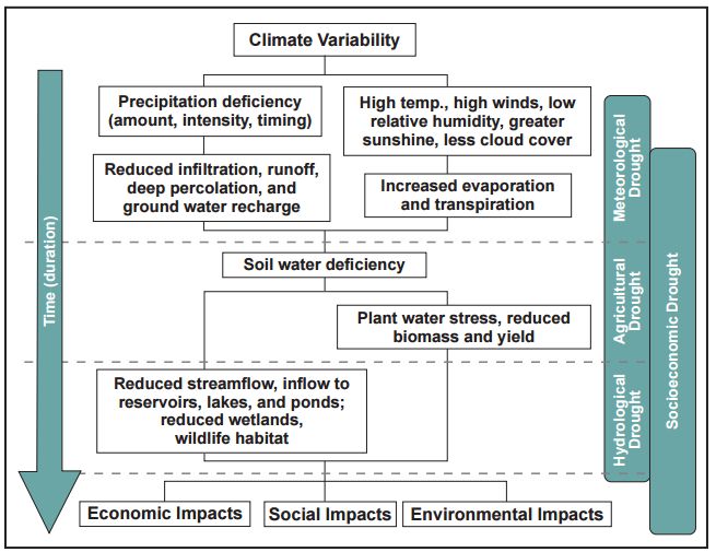
International Journal of Advanced Science and Technology
 Vol. 29, No. 7, (2020), pp. 13507 - 13525

Table 3: ANOVA test results

Given that these stations were different, a non-parametric K-means cluster analysis was applied to
group them into homogenous clusters. Table 4 shows three groupings where Johannesburg Zoological
Gardens (JZG) formed a single member group.

Table 4: K-means clustering results

 Cluster Weather station Gauteng
 1 Johannesburg Zoological Gardens (JZG)
 2 Irene, Vereeniging RWB (VRWB), Jan Smuts WK (JSWK)
 Johannesburg Turffontein (JT), Pretoria Burgers park (PBP), Randfontein
 3 (R)

 Johannesburg Zoological garden
 Mk, p-value=0.6607
 1350
 Annual rainfall (mm)

 1150

 950

 750

 550

 350
 1984

 1992

 2000

 2008

 2016
 1954
 1956
 1958
 1960
 1962
 1964
 1966
 1968
 1970
 1972
 1974
 1976
 1978
 1980
 1982

 1986
 1988
 1990

 1994
 1996
 1998

 2002
 2004
 2006

 2010
 2012
 2014

 Time (years)

Figure 3: Johannesburg Zoological Gardens (JZG) annual rainfall graph

ISSN: 2005-4238 IJAST
Copyright ⓒ 2020 SERSC
 13518

International Journal of Advanced Science and Technology
 Vol. 29, No. 7, (2020), pp. 13507 - 13525

 Jonnesburg Turffontein
 Mk, p-value=0.2086
 1400
 Annual rainfall (mm)

 1200

 1000

 800

 600

 400

 1974

 1986

 2008
 1954
 1956
 1958
 1960
 1962
 1964
 1966
 1968
 1970
 1972

 1976
 1978
 1980
 1982
 1984

 1988
 1990
 1992
 1994
 1996
 1998
 2000
 2002
 2004
 2006

 2010
 2012
 2014
 2016
 Time (years)

 Figure 4: Johannesburg Turffontein (JT) annual rainfall graph
 Pretoria Burgers Park
 Mk, p-value=0.2804
 1300
 Annual rainfall (mm)

 1100
 900
 700
 500
 300
 1974

 1984

 2006

 2016
 1954
 1956
 1958
 1960
 1962
 1964
 1966
 1968
 1970
 1972

 1976
 1978
 1980
 1982

 1986
 1988
 1990
 1992
 1994
 1996
 1998
 2000
 2002
 2004

 2008
 2010
 2012
 2014
 Time (years)

 Figure 5: Pretoria Burgers park (PBP) annual rainfall graph
 Irene
 Mk, p-value=0.2725
 1200
 Annual rainfall (mm)

 1000
 800
 600
 400
 1958

 1972

 1984

 2010
 1954
 1956

 1960
 1962
 1964
 1966
 1968
 1970

 1974
 1976
 1978
 1980
 1982

 1986
 1988
 1990
 1992
 1994
 1996
 1998
 2000
 2002
 2004
 2006
 2008

 2012
 2014
 2016

 Time (years)

 Figure 6: Irene (I) annual rainfall graph

ISSN: 2005-4238 IJAST
Copyright ⓒ 2020 SERSC
 13519

International Journal of Advanced Science and Technology
 Vol. 29, No. 7, (2020), pp. 13507 - 13525

 Vereeniging RWB
 Mk, p-value=0.1004
 1050
 Annual ainfall (mm)

 850
 650
 450
 250
 1964

 1974

 1990

 2016
 1954
 1956
 1958
 1960
 1962

 1966
 1968
 1970
 1972

 1976
 1978
 1980
 1982
 1984
 1986
 1988

 1992
 1994
 1996
 1998
 2000
 2002
 2004
 2006
 2008
 2010
 2012
 2014
 Time (years)

 Figure 7: Vereeniging RWB (VRWB) annual rainfall graph
 Randfontein
 Mk, p-value=0.7756
 1300
 Annual rainfall (mm)

 1100
 900
 700
 500
 300
 100
 1966

 1976

 1986

 2014
 1954
 1956
 1958
 1960
 1962
 1964

 1968
 1970
 1972
 1974

 1978
 1980
 1982
 1984

 1988
 1990
 1992
 1994
 1996
 1998
 2000
 2002
 2004
 2006
 2008
 2010
 2012

 2016
 Time (years)

 Figure 8: Randfontein (R) annual rainfall graph
 Jan Smuts WK
 Mk, p-value=0.3610
 1200
 Annual rainfall (mm)

 1000
 800
 600
 400
 1958

 1964

 1990

 1996
 1954
 1956

 1960
 1962

 1966
 1968
 1970
 1972
 1974
 1976
 1978
 1980
 1982
 1984
 1986
 1988

 1992
 1994

 1998
 2000
 2002
 2004
 2006
 2008
 2010
 2012
 2014
 2016

 Time (years)

 Figure 9: Jan Smuts WK (JSWK) annual rainfall graph

ISSN: 2005-4238 IJAST
Copyright ⓒ 2020 SERSC
 13520

International Journal of Advanced Science and Technology
 Vol. 29, No. 7, (2020), pp. 13507 - 13525

 Pretoria Purification
 Mk, p-value=0.5065
 1250
 Annual Rainfall (mm)

 1050
 850
 650
 450
 250
 1964

 1978

 2014
 1954
 1956
 1958
 1960
 1962

 1966
 1968
 1970
 1972
 1974
 1976

 1980
 1982
 1984
 1986
 1988
 1990
 1992
 1994
 1996
 1998
 2000
 2002
 2004
 2006
 2008
 2010
 2012

 2016
 Time (years)

 Figure 10: Pretoria Purification (PP) annual rainfall graph

Figures 3 to 10 shows the graphs of all stations’ rainfall and their Mann Kendall’s trend test results. In
all stations the p-values were found to be greater than 0.05 significance level. This implied that there
were trends present in the datasets hence neither increasing nor decreasing patterns. From the three
clusters three randomly selected stations were used to analyse the return levels of rainfall in the study
area. Tables 5 to 6 show that results of Probability of non-exceedance, return period, estimated
annual rainfall and drought category by standardised precipitation drought index (SPI). For all the
stations, there is a 50% chance (2 years return period) of getting a below normal rainfall that will
result in normal drought conditions.

Table 5: Johannesburg Zoological garden
Probability of non- Return period (Tx) Estimated annual Drought category
exceedance (Px) % (yrs) rainfall (mm) by (SPI)
90 1.11 1119 1.510
80 1.25 971.3 0.933
50 2 777.5 0.025
20 5 622 -0.885
Table 6: Johannesburg Turffontein
Probability of non- Return period (Tx) Estimated annual Drought category by
exceedance (Px) % (yrs) rainfall (mm) (SPI)
90 1.11 995.2 1.433
80 1.25 884.8 0.902
50 2 715.4 -0.066
20 5 604.1 -0.836
Table 7: Irene
Probability of non- Return period (Tx) Estimated annual Drought category
exceedance (Px) % (yrs) rainfall (mm) by (SPI)
90 1.11 905.8 1.315
80 1.25 844.7 0.964
50 2 703.0 0.043
20 5 574.3 -0.971

ISSN: 2005-4238 IJAST
Copyright ⓒ 2020 SERSC
 13521

International Journal of Advanced Science and Technology
 Vol. 29, No. 7, (2020), pp. 13507 - 13525

Conclusion and recommendations

In conclusion, the South African construction sector accounts for 11% of the total employment, thus
contributing approximately 4% of the country’s Gross Domestic Product (GDP). However, severe
unpredictable weather patterns can send this sector’s costs skyrocketing and revenue spiralling.
Construction industry is said to be a good indicator for economic growth. The aim of this current
study was to assess rainfall variability in the current rapidly changing climate regime, to set an avenue
for businesses’ opportunities and risk reduction adaptation measures in order to keep this industry in
the market. Annual rainfall data sets from eight weather stations were collected from an online source
for analysis. A non-parametric test, Pettitt’s homogeneity and Shapiro-Wilk tests for data stationarity
and normality respectively were deployed. A further Mann Kendall’s trend test was used to detect if
any monotonic trend patterns were existent in the data sets. The probability of non-exceedance and
return level periods were computed for each station. ANOVA test revealed all stations statistically
different in rainfall patterns. The major results for this study, was that (i) no statistically significant
decreasing patterns were observed over all candidate stations (ii), for every 2 to 5-year return periods,
all stations are to experience near-normal drought conditions as computed from Standardised
Precipitation Index (SPI). Given the frequent and intense drought episodes in South Africa and other
parts of the world, Gauteng province remains a relatively conducive environment for construction
business projects.

 References
 1. Abarca del Rio, R., Gambis, D., Salstein, D., Nelson, P., & Dai, A. (2003). Solar activity and
 earth rotation variability. Journal of Geodynamics, 36(3), 423–443.
 https://doi.org/10.1016/S0264-3707(03)00060-7
 2. Abdulmalek, A., Asheikh & Tarawneh, Q.Y. 2013. An analysis of Dry spell patterns Intensity
 3. and duration in Saudi Arabia. Middle East Journal of Scientific Research. 13(3): 314-327.

 4. Abraham, B., & Yatawara, N. (1988). a Score Test for Detection of Time Series Outliers.
 Journal of Time Series Analysis, 9(2), 109–119. https://doi.org/10.1111/j.1467-
 9892.1988.tb00458.x
 5. Andreadis, K. 2005. Trends in 20th century drought characteristics over the continental
 UnitedStates.http://www.hydro.washington.edu/Lettenmaier/Presentations/2005/andr
 eadis_UBCUW_2005.pdf. Date of access: 20 Oct. 2019.

 6. Ali, W., & Ali, B. W. (2011). Drought and drought mangement.
 7. Choi, J., An Prof., S. Il, Yeh, S. W., & Yu, J. Y. (2013). ENSO-like and ENSO-induced
 tropical pacific decadal variability in CGCMs. Journal of Climate, 26(5), 1485–1501.
 https://doi.org/10.1175/JCLI-D-12-00118.1
 8. Des Jardins, D. 2012. Incorporating drought risk from climate change into california water
 9. planning.http://www.waterboards.ca.gov/waterrights/water_issues/programs/bay_delta/docs/c
 omments111312/deirdre_desjardins_2.pdf. Date of access: 01 Oct. 2019.

 10. Do Amaral Cunha, A. P. M., Marchezini, V., Lindoso, D. P., Saito, S. M., & Dos Santos
 Alvalá, R. C. (2019). The challenges of consolidation of a drought-related disaster risk
 warning system to Brazil. Sustentabilidade Em Debate, 10(1), 43–59.
 https://doi.org/10.18472/SustDeb.v10n1.2019.19380
ISSN: 2005-4238 IJAST
Copyright ⓒ 2020 SERSC
 13522

International Journal of Advanced Science and Technology
 Vol. 29, No. 7, (2020), pp. 13507 - 13525

 11. Francisco, A. R. L. (2013). 済無No Title No Title. Journal of Chemical Information and
 Modeling, 53(9), 1689–1699. https://doi.org/10.1017/CBO9781107415324.004
 12. Gaas, A. O. (2018). Impact Assessment of Recurrent Droughts on Agricultural and Pastoral
 Communities in Somaliland. 6(4), 1411–1421.
 13. Ghormar, B. K. T. B. R. (2014). Solar Interplanetary and Geomagnetic Activity in Solar
 Cycle 23. 2(07), 1–2.
 14. Granzow-de la Cerda, Í., Lloret, F., Ruiz, J. E., & Vandermeer, J. H. (2012). Tree mortality
 following ENSO-associated fires and drought in lowland rain forests of Eastern Nicaragua.
 Forest Ecology and Management, 265, 248–257. https://doi.org/10.1016/j.foreco.2011.10.034
 15. Hlalele, B.M. 2016. A probabilistic approach to drought frequency analysis in Mafube Local
 16. Municipality, South Africa. Research Journal of Pharmaceutical, Biological and Chemical
 17. Sciences, 7(6): 3008-3015.

 18. Hosseinzadeh Talaee, P., Kouchakzadeh, M., & Shifteh Some’e, B. (2014). Homogeneity
 analysis of precipitation series in Iran. Theoretical and Applied Climatology, 118(1–2), 297–
 305. https://doi.org/10.1007/s00704-013-1074-y
 19. Jordan, A. J. (2017). Vulnerability, Adaptation to and Coping with Drought: The Case of
 Commercial and Subsistence Rainfed Farming in the Eastern Cape. WRC Report Number:
 TT716/1/17. In Water Research Commission.
 20. Keil, A., Zeller, M., Wida, A., Sanim, B., & Birner, R. (2008). What determines farmers’
 resilience towards ENSO-related drought? An empirical assessment in Central Sulawesi,
 Indonesia. Climatic Change, 86(3–4), 291–307. https://doi.org/10.1007/s10584-007-9326-4
 21. Khan, S. M., & Gomes, J. (2019). Drought in Ethiopia: A Population Health Equity Approach
 to Build Resilience for the Agro-Pastoralist Community. Global Journal of Health Science,
 11(2), 42. https://doi.org/10.5539/gjhs.v11n2p42
 22. Kliewer, J., & Mertins, A. (1997). Design of paraunitary oversampled cosine-modulated filter
 banks. ICASSP, IEEE International Conference on Acoustics, Speech and Signal Processing -
 Proceedings, 3, 2073–2076. https://doi.org/10.1109/icassp.1997.599355
 23. Lobato, I. N., & Velasco, C. (2004). A simple test of normality for time series. Econometric
 Theory, 20(4), 671–689. https://doi.org/10.1017/S0266466604204030
 24. Méthy, M., Damesin, C., & Rambal, S. (1996). Drought and photosystem II activity in two
 Mediterranean oaks. Annales Des Sciences Forestières, 53(2–3), 255–262.
 https://doi.org/10.1051/forest:19960208
 25. Minckley, R. L., Roulston, T. H., & Williams, N. M. (2013). Resource assurance predicts
 specialist and generalist bee activity in drought. Proceedings of the Royal Society B:
 Biological Sciences, 280(1759). https://doi.org/10.1098/rspb.2012.2703
 26. Minnis, C. M. (1958). Solar activity and the ionosphere. Nature, 181(4608), 543–544.
 https://doi.org/10.1038/181543a0
 27. Nagamuthu, P., & Rajendram, K. (2015). Occurrences of Flood Hazards in the Northern
 Region of Sri Lanka. J. S. Asian Stud, 03(03), 363–376. Retrieved from
 http://www.escijournals.net/JSAS
 28. National Drought Mitigation Center (NDMC), 2012. What is drought?
 29. http://drought.unl.edu/DroughtBasics/WhatisDrought.aspx. Date of access: 11 Nov. 2019.

 30. Olivares Campos, B. O. (2016). Análisis temporal de la sequía meteorológica en localidades
 semiáridas de Venezuela. UGCiencia, 22(1), 11. https://doi.org/10.18634/ugcj.22v.1i.481
 31. Orlando Olivares, B., & Zingaretti, M. L. (2018). Análisis de la sequía meteorológica en
 cuatro localidades agrícolas de Venezuela mediante la combinación de métodos
 multivariados. UNED Research Journal, 10(1), 181–192.
 https://doi.org/10.22458/urj.v10i1.2026
 32. Praveen, D., Ramachandran, A., Jaganathan, R., Krishnaveni, E., & Palanivelu, K. (2016).
 Projecting droughts in the purview of climate change under RCP 4.5 for the coastal districts
 of South India. Indian Journal of Science and Technology, 9(6).
 https://doi.org/10.87677/ijst/2016/v9i6/87677
ISSN: 2005-4238 IJAST
Copyright ⓒ 2020 SERSC
 13523

International Journal of Advanced Science and Technology
 Vol. 29, No. 7, (2020), pp. 13507 - 13525

 33. Prokurat, S. (2015). Drought and water shortages in Asia as a threat and economic problem.
 Journal of Modern Science, 26(3), 235–250.
 34. Rahmat, S. N., Jayasuriya, N., & Bhuiyan, M. (2012). Trend analysis of drought using
 Standardised Precipitation Index (SPI) in Victoria, Australia. Proceedings of the 34th
 Hydrology and Water Resources Symposium, HWRS 2012, (1996), 441–448.
 35. Román-Cuesta, R. M. (2007). Environmental and human factors influencing fire trends in
 ENSO and non-ENSO years in tropical Mexico (Ecological Application (2003) 13, (1177-
 1192)). Ecological Applications, 17(5), 1555. https://doi.org/10.1890/1051-
 0761(2007)17[1555:E]2.0.CO;2
 36. Potop, V., Boroneant, C., Možný, M., Štěpánek, P. & Skalák, P. 2013. Observed
 spatiotemporal characteristics of drought on various time scales over the Czech Republic.
 Theoretical and Applied Climatology. 112(4): 1-21.

 37. Ryu, J. H., Svoboda, M. D., Lenters, J. D., Tadesse, T., & Knutson, C. L. (2010). Potential
 extents for ENSO-driven hydrologic drought forecasts in the United States. Climatic Change,
 101(3), 575–597. https://doi.org/10.1007/s10584-009-9705-0
 38. Siingh, D., Singh, R. P., Singh, A. K., Kulkarni, M. N., Gautam, A. S., & Singh, A. K. (2011).
 Solar Activity, Lightning and Climate. Surveys in Geophysics, 32(6), 659–703.
 https://doi.org/10.1007/s10712-011-9127-1
 39. Sobrino, J.A. & Julien, Y., 2011. Global trends in NDVI-derived parameters obtained from
 GIMMS data. International Journal of Remote Sensing, 32(15): 4267- 4279.

 40. Solheim, J.-E., Stordahl, K., & Humlum, O. (2011). Solar Activity and Svalbard
 Temperatures. Advances in Meteorology, 2011, 1–8. https://doi.org/10.1155/2011/543146
 41. Tadić, T., Dadić, T. & Bosak, M. 2015. Comparison of different drought assessment methods
 in continental Croatia. DOI: 10.14256/JCE.1088.2014. Date of access: 20 Sep. 2019.

 42. Tan, B., & Ylmaz, K. (2002). Markov chain test for time dependence and homogeneity: An
 analytical and empirical evaluation. European Journal of Operational Research, 137(3), 524–
 543. https://doi.org/10.1016/S0377-2217(01)00081-9
 43. Technology, B., & Bay, H. K. (2001). Department of Electrical and Computer Engineering,
 University of Patras, 26500 Rion, Patras Department of Electrical and Computer
 Engineering, University of Patras 1 Computer Science Department, University of Ioannina.
 (October).
 44. Tefera, A. S., Ayoade, J. O., & Bello, N. J. (2019). Comparative analyses of SPI and SPEI as
 drought assessment tools in Tigray Region, Northern Ethiopia. SN Applied Sciences, 1(10).
 https://doi.org/10.1007/s42452-019-1326-2
 45. Van Niekerk, D. 2011. Introduction to disaster risk reduction. Potchefstroom: The African
 Centre for Disaster Studies NWU Potchefstroom.

 46. Verma, M. K., Verma, M. K., Yadu, L. K., & Murmu, M. (2016). Drought analysis in the
 seonath river basin using reconnaissance drought index and standardised precipitation index.
 International Journal of Civil Engineering and Technology, 7(6), 714–719.
 47. Xiao, J., & Zhuang, Q. (2007). Drought effects on large fire activity in Canadian and Alaskan
 forests. Environmental Research Letters, 2(4), 1–6. https://doi.org/10.1088/1748-
 9326/2/4/044003
 48. Yuliang, Z., Li, L., Ping, Z., Juliang, J., Jianqiang, L. & Chengguo, W. 2014. Identification
 of drought and frequency analysis of drought characteristics based on palmer drought severity
 index model. The Chinese Society of Agricultural Engineering. 30(23):174-184.

 49. Yusof, F., Hui-Mean, F., Suhaila, J., Yusop, Z., & Ching-Yee, K. (2014). Rainfall
 characterisation by application of standardised precipitation index (SPI) in Peninsular
ISSN: 2005-4238 IJAST
Copyright ⓒ 2020 SERSC
 13524

International Journal of Advanced Science and Technology
 Vol. 29, No. 7, (2020), pp. 13507 - 13525

 Malaysia. Theoretical and Applied Climatology, 115(3–4), 503–516.
 https://doi.org/10.1007/s00704-013-0918-9

ISSN: 2005-4238 IJAST
Copyright ⓒ 2020 SERSC
 13525