Inter-annual Climate Variability and Vegetation Dynamic in the Upper Amur (Heilongjiang) River Basin in Northeast Asia - IOPscience
←
→
Page content transcription
If your browser does not render page correctly, please read the page content below
Environmental Research Communications

LETTER • OPEN ACCESS

Inter-annual Climate Variability and Vegetation Dynamic in the Upper
Amur (Heilongjiang) River Basin in Northeast Asia
To cite this article: Guangyong You et al 2020 Environ. Res. Commun. 2 061003

View the article online for updates and enhancements.

                               This content was downloaded from IP address 176.9.8.24 on 30/09/2020 at 09:12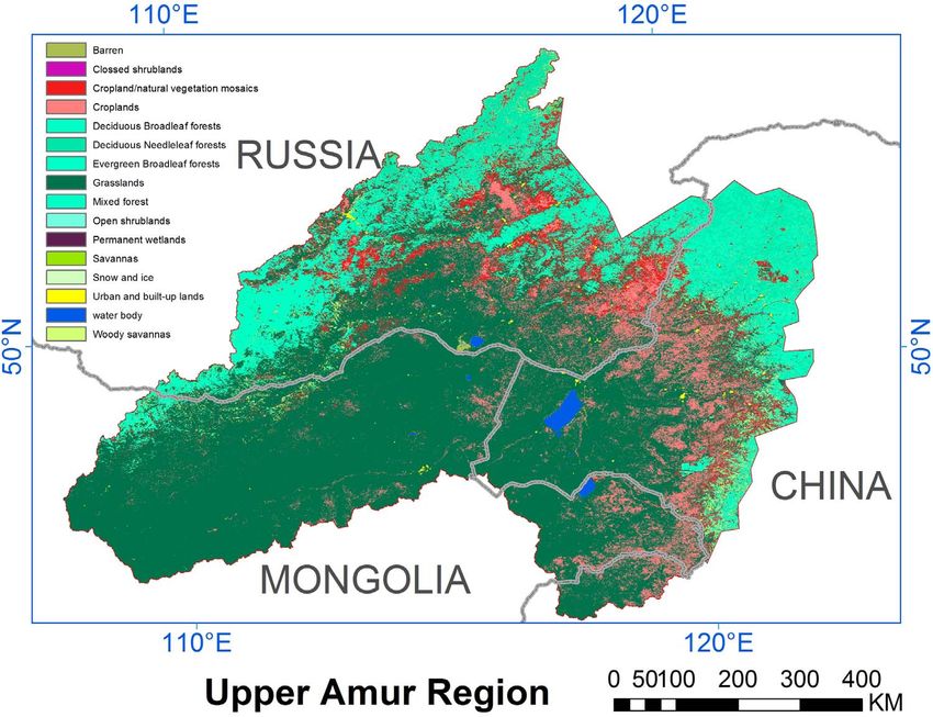
Environ. Res. Commun. 2 (2020) 061003 https://doi.org/10.1088/2515-7620/ab9525
LETTER
Inter-annual Climate Variability and Vegetation Dynamic in the
OPEN ACCESS
Upper Amur (Heilongjiang) River Basin in Northeast Asia
RECEIVED
25 November 2019
Guangyong You1,2 , M Altaf Arain2, Shusen Wang3, Shawn McKenzie2, Bing Xu2, Yaqian He4 , Dan Wu1,
REVISED
24 April 2020
Naifeng Lin1, Jixi Gao1 and Xiru Jia5
1
Nanjing Institute of Environment Sciences, Ministry of Ecology and Environment, Nanjing, Jiangsu, 210042, People’s Republic of China
ACCEPTED FOR PUBLICATION 2
20 May 2020 School of Geography and Earth Sciences and McMaster Centre for Climate Change, McMaster University, Hamilton, Ontario L8S4K1,
Canada
PUBLISHED 3
5 June 2020
Canada Centre for Remote Sensing, Natural Resources Canada, Ottawa, Ontario K1A0E4, Canada
4
Department of Geology and Geography, West Virginia University, Morgantown, WV 26506, United States of America
5
School of Environment & Natural Resources, Renmin University of China, Beijing, 100872, People’s Republic of China
Original content from this
work may be used under E-mail: gjx@nies.org
the terms of the Creative
Commons Attribution 4.0 Keywords: climate change, vegetation response, NDVI variability, growing season length, Amur River
licence.
Supplementary material for this article is available online
Any further distribution of
this work must maintain
attribution to the
author(s) and the title of
the work, journal citation Abstract
and DOI. Long-term (1982–2013) datasets of climate variables and Normalized Difference Vegetation Index
(NDVI) were collected from Climate Research Union (CRU) and GIMMS NDVI3g. By setting the
NDVI values below the threshold of 0.2 as 0, NDVI_0.2 was created to eliminate the noise caused by
changes of surface albedo during non-growing period. TimeSat was employed to estimate the growing
season length (GSL) from the seasonal variation of NDVI. Statistical analyses were conducted to reveal
the mechanisms of climate-vegetation interactions in the cold and semi-arid Upper Amur River Basin
of Northeast Asia. The results showed that the regional climate change can be summarized as warming
and drying. Annual mean air temperature (T) increased at a rate of 0.13 °C per decade. Annual
precipitation (P) declined at a rate of 18.22 mm per decade. NDVI had an insignificantly negative
trend, whereas, NDVI_0.2 displayed a significantly positive trend (MK test, p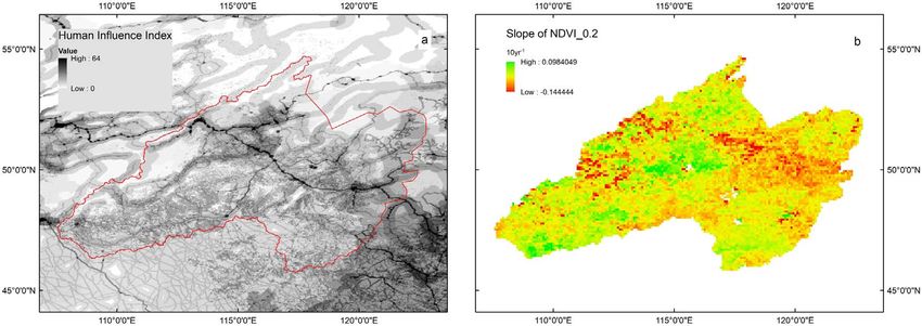
Environ. Res. Commun. 2 (2020) 061003
activity were related to regional climate warming (Fensholt et al 2012, Cong et al 2013, Zelikova et al 2015).
However, the positive effect of climate warming on vegetation dynamics was insignificant despite the
pronounced increase in temperature (Garonna et al 2014). In addition, there have been weakening relationships
between vegetation dynamics and temperature at continental scales (Piao et al 2014), which complicates our
understanding of vegetation responses to climate change in regions characterized as both cold and arid/
semi-arid.
Furthermore, the co-linearity among climate variables can mislead the conclusions of statistical analyses and
results in diversified trends and pseudo driving factors (Wu et al 2015, Seddon et al 2016). For example, studies
on temporal variations of vegetation activities in cold and arid/semi-arid region of northeastern Asia provided
controversial conclusions. Shinoda and Nandintsetseg (2011) investigated the soil moisture and plant
phenology in Mongolian grassland and highlighted the availability of water in controlling vegetation activities.
In contrast, Lin et al (2015) reported the insignificant relationship between precipitation and vegetation
dynamics. To provide further controversy, Mohammat et al (2013) concluded temperature variability was the
dominant factor in controlling the vegetation growth in northeast Asia, which complicates our understanding of
the relationship between climate change and vegetation response.
The upper stream of Amur River is a typical region in north-eastern Asia characterized as both cold and dry
(Simonov and Egidarev 2017). Vegetation growth and phenological change are vulnerable to climate variability
(Shinoda and Nandintsetseg 2011, Mohammat et al 2013, Lin et al 2015). Besides the controversy about the
driving factors, previous studies chose political borders as their study boundaries disregarding the natural
watershed and basin boundaries. As the climate change will pose a threat to both ecosystem function and the
provision of ecosystem services, a detailed analysis of the relationship between climate change and vegetation
response over the past decades will be helpful to further our understanding of natural processes in this region.
In this study, three decades (1982 to 2013) of climate variables and vegetation dynamics in the upper Amur
River basin in northeastern Asia were examined to address the following questions: (1) what are the regional
patterns of climate change and vegetation dynamics in this region?(2) What are the roles of climate variables
and human activities, if any, in controlling the vegetation dynamics?(3) What is the contribution of each
climate variable on influencing the vegetation dynamics?
2. Data source and methods
2.1. Study site
The upper stream of the Amur River is located in northeastern Asia and the watershed includes territories of
three countries: Russia, Mongolia, and China (figure 1). The climate of Amur basin is influenced by East Asian
monsoon and characterized as warm and moderate humid summer alternated with cold and dry winter.
Herbaceous plants, such as Stipa krylovii, Stipa baicalensi, and Leymus chinensis are dominant in this area
(Simonov and Egidarev 2017). Based on the long-term climatic observation from Manzhouli station (49°36′0′N,
117°25′59.99′E) located approximately in the center of the study area, the annual mean temperature in the
watershed is −0.6 °C with −23.3 °C in coldest month and 19.6 °C in warmest month, and the mean total annual
precipitation is 303.4 mm with 88.2% delivered during the summer of the monsoon season (June-September).
The aridity index, the ratio of mean annual precipitation to mean annual potential evapotranspiration proposed
by United Nations Environment Programme (UNEP), is 0.49 in Manzhouli station. According to Köppen
classification of climates (Köppen 1936), the study area is situated between cold semi-arid climate (Bsk) and
Monsoon-influenced warm-summer humid continental climate (Dwb) and Monsoon-influenced subarctic
climate (Dwc).
This region was characterized as scarce of water but high ecological values (Simonov and Egidarev 2017). It
possesses tremendous biodiversity with at least 600 species of vascular plants, 30 fish species, at least 303 bird
species and about 35 mammal species. Grassland, rivers, lakes and wetlands provide a variety of habitats and
niches for endangered species. As a result, the Amur River basin was identified as one of the world’s 200 most
valuable wilderness places. Hulun Lake (covering approximately 2,339 km2) located in the center of upper
stream of Amur, is enrolled in the Wetlands of International Importance (United Nations’ Ramsar List).
For this study, we obtained the watershed boundary of Amur River (Heilongjiang) from HydroSHEDS
(https://hydrosheds.cr.usgs.gov/) and intercepted the watershed boundary with approximately 1000 m
elevation contour extracted from ETOPO1 model (Amante and Eakins 2009). This incepted sub-basin area is
687,675 km2 with low population density of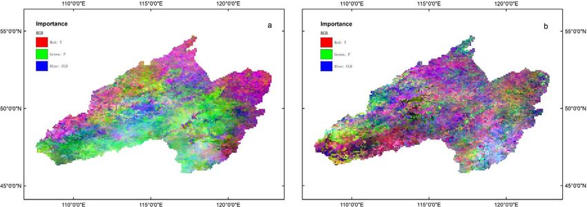
Environ. Res. Commun. 2 (2020) 061003

  Figure 1. The location of the study area and the spatial distribution of land use types (MODIS MCD12Q1) within the upper stream of
  Amur River basin.

2.2. Data source
2.2.1. NDVI data
The Normalized Difference Vegetation Index (NDVI) has been used extensively for reflections of vegetation
dynamics and plant phenology (Pinzon and Tucker 2014). The Global Vegetation Inventory Modeling and
Mapping Studies (GIMMS) NDVI3g dataset (1982–2013) was used to reveal the spatial and temporal
distribution of vegetation dynamics (https://ecocast.arc.nasa.gov/). The GIMMS NDVI3g dataset was
normalized for sensor calibration loss, orbital drift, and atmospheric effects (e.g. volcanic eruptions). We
followed He et al (2017) method (removing data that was flagged 3 to 7—corresponding to bad data quality) to
obtain the long-term NDVI images with a spatial resolution of 1/12° at 15-day intervals.
    As the threshold of 0.2 in NDVI is widely considered representative for the onset/offset of plant growing
period (Esau et al 2016, Liang et al 2016), we developed an index of NDVI_0.2 by setting the pixel value below the
threshold of 0.2 to zero. NDVI_0.2 can be more effective in representing the vegetation growth and dynamic as a
result of the influence of noise, such as snow cover during winter, is removed.

2.2.2. Climate data
The Climatic Research Unit (CRU: University of East Anglia Climatic Research Unit, 2008, http://cru.uea.ac.
uk/data) processed scheme harmonized station-based observation data sources to generate reliable estimates of
global climate with spatial interpolation at 0.5° grid resolution (Mitchell and Jones 2005). The dataset CRU TS
was taken for climate analysis as it provided time series of several climate variables with high accuracy (Harris
et al 2014). We extracted 7 climate variables, including the Palmer Drought Severity Index (PDSI) (Palmer 1965)
calculated by a physical water balance model, from grids corresponding to the study area at monthly interval
from 1982 to 2013. The CRU-extracted data at Manzhouli site (49°36′0′N, 117°25′59.99′E) were validated by
ground meteorological observations collected from China Meteorological Data Service Center (http://
nmic.cn/).
     The PDSI is the most prominent index of meteorological drought (Dai 2011). It incorporates antecedent
precipitation, moisture supply, and moisture demand into a hydrological accounting system, with the intent to
measure the cumulative departure (relative to local mean conditions) in atmospheric moisture supply and
demand at the surface.
     Warmth index (WMI) and cold index (CDI) are considered as the key bio-climatic factors that influence
plant growth, species distribution and terrestrial net primary production (Kira 1945, Wen et al 2018). In this
study, WMI and CDI were prepared for each pixel using equations (1) and (2), which count the annual sum of

                                                      3
Environ. Res. Commun. 2 (2020) 061003
positive and negative differences between monthly means and 5 °C. As the vegetation activity is mostly
influenced by coldness before the growing season (You et al 2019), the CDI in this study is counting the negative
temperature difference (T−5 °C) between two consecutive summers.
WMI = åT - 5 (T 5) (1)
CDI = - å 5 - T (T < 5) (2)
The Potential evapotranspiration (PET) is calculated from a variant of the Penman–Monteith formula
(http://fao.org/docrep/X0490E/x0490e06.htm) using TMP, TMN, TMX, VAP, CLD and time invariant values
of wind speed (i.e. the same 1961–1990 monthly values for each month in each year).
900
0.408D (Rn - G ) + g T + 273.16 U (e a - e d )
PET = (3)
D + g (1 + 0.34U )
PET: reference crop evapotranspiration (mm); Rn: net radiation (MJ m−2); G: soil heat flux (MJ m−2); T:
average temperature (°C); U: windspeed (m s−1); (ea − ed): vapour pressure deficit (kPa); Δ: slope of the vapour
pressure curve (kPa °C−1); γ: psychrometric constant (kPa °C−1) ; 900: coefficient for the reference crop (kJ−1 kg
K); 0.34: wind coefficient for the reference crop. Detailed description of the parameters above can be found in
Allen et al (1998).
2.2.3. Growing season length
The TIMESAT program was employed in this study to smooth the raw data and extract seasonality parameters
(Eklundh and Jönsson 2015). For each pixel, the median filtering method was applied to remove spikes and
outliers of NDVI. Then, Savitzky-Golay method was applied to generate a smoothed NDVI time series, from
which seasonality parameters were extracted (Savitzky and Golay 1964, Eklundh and Jönsson 2015).
For each pixel, time series of 768 anomalies (32 year×12 month×2 images/month) was extracted. All of
the settings of parameters followed the previous studies (Chen et al 2004, He et al 2017). The start of growing
season (SOS) is the time for which the left edge has increased to 50% of the seasonal amplitude measured from
the left minimum level. The time for the end of the season (EOS) is the time for which the right edge has
decreased to 50% of the seasonal amplitude measured from the right minimum level. The growing season length
(GSL) is the time from the start to the end of the growing season.
To validate the GSL extracted by TIMESAT, we conducted a comparison between the TIMESAT extracted
GSL and the available phenological records reported at Hulunbeier station (49°19′N, 119°55′E) (Zhou and
Liu 2017). Good agreement suggests the TIMESAT is applicable in this study (table S2; figure S1).
2.2.4. Human influence index
As the regional climate change was combined with human activity, a comparison between the spatial
distribution of NDVI trend and human activity is helpful in understanding the role of human activity in the
regional climate-vegetation relationship. The Global Human Influence Index (HII) Dataset was collected from
Socioeconomic Data and Applications Center, NASA’s Earth Observing System Data and Information System
(EOSDIS)—Hosted by CIESIN at Columbia University (http://sedac.ciesin.columbia.edu/wildareas/)
(Columbia Wildlife Conservation Society and Center for International Earth Science Information
Network 2005). The HII was created from nine global data layers covering human population pressure
(population density), human land use and infrastructure (built-up areas, nighttime lights, land use/land cover),
and human access (coastlines, roads, railroads, navigable rivers).
Atmospheric CO2 concentrations at Mauna Loa observatory was obtained from National Oceanic and
Atmospheric Administration Earth System Research Laboratory (NOAA ESRL; http://esrl.noaa.gov/gmd/
ccgg/trends). We ignored latitudinal differences in CO2 concentration as these are small compared to the signal
of inter annual variation. Table 1 displayed all of the data sources and abbreviations.
2.3. Statistical analysis
2.3.1. Trend analysis
The trend of each variable was analyzed using the Mann–Kendall test (Mann 1945, Kendall 1975, McLeod et al
2012). A pre-whitening procedure (MK-TFPW) was applied to reduce the influence of autocorrelation on the
significance of Mann–Kendall test results (Mann 1945, Yue and Wang 2002). Positive tau value from MK-TFPW
test indicates an increasing trend, whereas, negative tau represents a decreasing trend.
4Environ. Res. Commun. 2 (2020) 061003
Table 1. Abbreviations and data sources of climate variables, human influence index and vegetation activities (NDVI, NDVI_0.2 and GSL).
Abbreviation Variables Unit Source/Method
T Daily mean temperature °C CRU TS v4.01
TMX Daily maximum temperature °C CRU TS v4.01
TMN Daily minimum temperature °C CRU TS v4.01
P Precipitation mm CRU TS v4.01
PET Potential evapotranspiration mm CRU TS v3.23
PDSI Self-calibrating Palmer drought severity index — (Schrier et al 2013)
WMI Warmth index of Kira, accumulation of monthly T above a threshold of 5 °C °C month−1 (Ohsawa 1993)
CDI Cold index of Kira, accumulation of negative temperature difference between °C month−1 (Ohsawa 1993)
monthly T and a threshold of 5 °C
CLD Cloud Coverage % CRU TS v4.01
HII Human Influence Index — (EOSDIS, NASA)
CO2 Atmospheric CO2 concentrations ppm (ESRL, NOAA)
NDVI The Normalized Difference Vegetation Index — GIMMS NDVI3g
NDVI_0.2 NDVI above a threshold of 0.2 — GIMMS NDVI3g
GSL Vegetation growing season length days TIMESAT 3.2
2.3.2. Change point detection
To detect change points in these time series, the Mann–Whitney–Pettit test was conducted (Pettitt 1979). Each
variable was standardized to z-score with long-term mean and standard deviation. A low pass filter (10 years) of
the standardized time series was calculated to reveal the temporal pattern of time series fluctuation.
2.3.3. Correlation analysis
Correlation analyses between climatic variables and vegetation activities were conducted to reveal the driving
factors. Then partial correlation analyses were also conducted to reveal the relative importance among the
comparable climate variables.
2.3.4. Principal regression analysis
The climate variables were de-aggregated to match GIMMS NDVI3g both spatially and temporally. In each pixel
across the study area, all time series were transformed to z-score anomalies using long-term mean and standard
deviation, and then principal regression analyses were conducted following the procedure reported by Seddon
et al (2016). To present the results spatially, the relative importances of the climate variables were plotted using
color composition.
3. Results
3.1. Climate change and trend analyses
Figure 2 and table 2 display the 32-year trends of climatic variables and vegetation activities from 1982 to 2013.
Annual T increased insignificantly with a slope of 0.13 °C per decade (p=0.36), TMN increased insignificantly
with a slope of 0.09 °C per decade (p=0.50) and TMX also increased insignificantly with a slope of 0.17 °C per
decade (p=0.28), indicating the increased diurnal range of air temperature at the background of climate
warming. The increased seasonal range of temperature was revealed by the integrated effects of increased WMI
and decreased CDI.
The seasonal fluctuation of PET follows the of variation of T. The regional average annual PET is
702.50±32.75 mm which is about 2 times higher than annual P (349.58±65.11 mm). From 1982 to 2013,
annual P insignificantly declined at a rate of 18.22 mm per decade (p=0.14), whereas, annual PET significantly
increased at a rate of 17.35 mm per decade (p=0.04). CLD and PDSI displayed significant negative trend,
suggesting the increased solar radiation and aridity. Overall, the regional climate change was characterized as
warming and drying.
Results of the Mann–Whitney–Pettit test of climate variables and atmospheric CO2 concentration are
displayed in table 2. A significant change point in P occurred around the year 1998, when P shifted from a
moderate (insignificant) trend of 4.961 mm per decade (p=0.87) to a great (significant) slope of 78.52 mm per
decade (p=0.02). Similarly, this significant change point (around the year 1998) was also detected in humidity-
related climate variables (PET and PDSI). Temperature variation (T, TMN and TMX) displayed an insignificant
change point (around the year 1988) over the past decades.
5Environ. Res. Commun. 2 (2020) 061003
Figure 2. Annual values (cross), linear trends (solid lines) and low pass filter (10 years, dashed lines) of standardized climate variables
of T (a), P (b), WMI (c), NDVI (d) and GSL (e).
3.2. Vegetation dynamics
The long term average NDVI is 0.35 and has an insignificantly negative linear trend over the past three decades.
Whereas, NDVI_0.2 has a significantly positive MK trend (table 2). The average GSL was 135.2 days and
significantly increased with a slope of 2.94 days per decade (p=0.00).
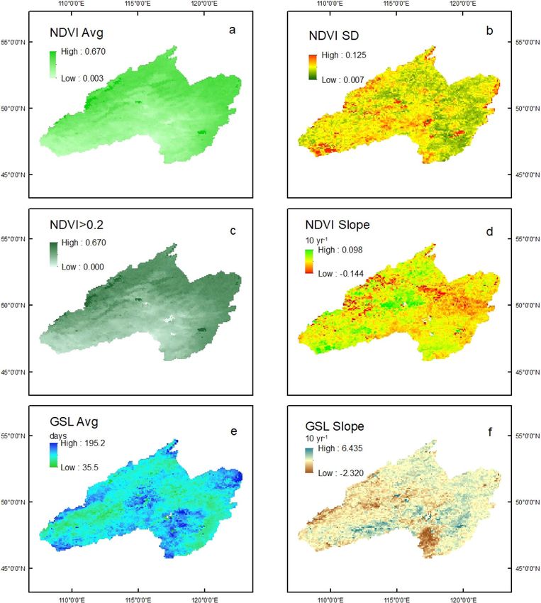
Figure 3 displayed the spatial distribution of averaged NDVI and GSL. Spatially, NDVI in the eastern region
(forest) displayed low inter-annual stand deviation, whereas, NDVI in grassland of the middle and western sub-
regions displayed considerable inter-annual variation (figure 3(b)). The pixels of positive NDVI trend were
mostly distributed in the middle of the region. Spatially, the average annual GSL in high elevated (forest) areas
were higher than the low land (steppe) located in the middle of the region. The positive GSL trend was mostly
distributed in the eastern sub-region, whereas, the negative GSL trend was mostly distributed in the
western part.
The spatial distribution of human influence did not overlap with negative NDVI trend (figure 4), suggesting
the negative NDVI trend can’t be explained by human activities exclusively.
6Environ. Res. Commun. 2 (2020) 061003
Table 2. Trend analyses of climate variables and vegetation activities (NDVI, NDVI_0.2 and GSL) in the upper Amur River basin.
WMI CDI CO2
Trend Analysis T (°C) TMX (°C) TMN (°C) (°C·month) (°C·month) CLD (%) P (mm) PET (mm) PDSI AI (ppm) NDVI (%) NDVI_0.2 (%) GSL (days)
MK-tau 0.044 0.089 0.061 0.552 −0.044 −0.274 −0.222 0.391 −0.403 −0.250 1.00 0.016 0.250 0.403
2-sided p value 0.733 0.486 0.638 0.000 0.733 0.028 0.077 0.002 0.001 0.046 0.000 0.909 0.046 0.001
7
pwmk-tau 0.045 0.058 0.077 0.251 −0.067 −0.268 −0.153 0.316 −0.209 −0.196 0.871 −0.006 0.170 0.256
Sen slope (per 10 yr) 0.068 0.125 0.891 2.836 0.861 −0.154 −23.022 18.69 −1.013 −0.043 17.425 0.035 0.402 3.331
Linear slope (per 10 yr) 0.127 0.165 0.090 2.957 −1.283 −0.128 −18.216 17.347 −0.836 −0.038 17.421 −0.049 0.337 2.943
2-sided p for linear 0.363 0.275 0.509 0.000 0.481 0.039 0.147 0.004 0.005 0.078 0.000 0.809 0.078 0.002
Slope
Change point year 1988 1988 1987 1997 1988 2002 1998 1996 1999 1988 1997 2002 1993 1998
2-sided p in change 0.351 0.376 0.339 0.000 0.402 0.018 0.039 0.025 0.003 0.351 0.000 0.327 0.215 0.002
point
Slope (before change) −1.019 −0.948 −2.151 2.405 −16.322 0.110 4.961 8.592 −0.102 0.000 14.679 0.706 0.502 1.245
2-sided p 0.507 0.577 0.065 0.035 0.130 0.257 0.873 0.563 0.858 0.997 0.000 0.022 0.513 0.332
Slope (after change) −0.186 −0.127 −0.246 −0.326 2.757 −0.067 78.524 7.504 0.316 −0.036 19.989 2.75 −0.081 −4.015
2-sided p 0.254 0.482 0.115 0.829 0.001 0.809 0.017 0.655 0.734 0.231 0.000 0.002 0.832 0.134Environ. Res. Commun. 2 (2020) 061003
Figure 3. Spatial distribution of annually averaged NDVI (a), stand deviation (SD) of NDVI (b), annually averaged NDVI_0.2 (c),
slope of NDVI (1982–2013) (d), annually averaged GSL (e) and slope of GSL (1982–2013) (f).
3.3. Correlation analyses
Correlation analyses revealed that T, TMX, TMN PET, CLD, CDI and WMI were of insignificant relationship
with NDVI (table 3), indicating the vegetation growth was insensitive to climate warming. As climate warming
has an effect of drying the air, NDVI_0.2 displayed significantly negative correlations with T, TMX, TMN, WMI
and PET. Contrast to the insignificant and negative roles of temperature regimes, both NDVI and NDVI_0.2 had
significantly positive correlations with P (p=0.04) and PDSI (p=0.02), suggesting the vegetation growth was
mostly sensitive to variation of moisture availability.
The GSL displayed significantly positive correlations with PET (p=0.04), TMX (p=0.04, Kendall
method) and WMI (p=0.00) but significantly negative correlations with P (p=0.02), PDSI (p=0.01),
suggesting the GSL was driven differently from the patterns of NDVI and NDVI_0.2. Partial correlation revealed
that GSL was mostly sensitive to WMI, whereas, NDVI and NDVI_0.2 displayed high sensitivities to both of
PDSI and WMI.
The atmospheric CO2 concentration displayed insignificant correlations with NDVI and NDVI_0.2
(table 3), suggesting the limited effect of carbon fertilization on plant growth. However, the significant
correlation between CO2 and GSL suggests a considerable influence of increased atmospheric CO2
concentration on plant phenological changes.
8Environ. Res. Commun. 2 (2020) 061003
Figure 4. The spatial distributions of HII (a), downloaded from Socioeconomic Data and Applications Center, NASA’s Earth
Observing System Data and Information System (EOSDIS)—Hosted by CIESIN at Columbia University (http://sedac.ciesin.
columbia.edu/wildareas/) and the spatial distribution of slope of NDVI_0.2 (b).
The atmospheric CO2 concentration displayed a persistent increase that differs from the inter-annual
variation of climate variables. Partial correlation analysis was conducted to compare the importances of
increased atmospheric CO2 and WMI, which were significantly correlated with GSL. The result showed that, the
partial correlation between CO2 and GSL is 0.150 (controlling WMI, p=0.420), whereas, the partial correlation
between WMI and GSL is 0.379 (controlling CO2, p=0.036). Therefore, WMI weigh higher importance than
CO2 in controlling the inter-annual variation of GSL.
These results of correlation analyses were confirmed by low pass filters (10 years) of their standardized time
series (figure 2). The fluctuation of standardized P had a similar temporal pattern with that of NDVI. And the
temporal fluctuation of standardized WMI had a similar pattern with that of GSL.
3.4. Principal regression analyses
Principal analysis of the climate variables revealed that the first 3 principals could explain 84.4% of the total
variance. Table 3 displayed the Pearson correlation coefficients between climate variables and the first 3
principal components (PC1, PC2 and PC3). The first principal (PC1) was highly correlated with temperature
regime (T, TMN, TMX), the second principal (PC2) was highly correlated with moisture conditions (P, PDSI),
and the third principal was highly correlated with CLD, suggesting the regional climate change can be
summarized as the changes of T, P and CLD. These three principal components represented the temperature,
moisture and radiation conditions which were widely considered as driving factors for vegetation activities.
Principal regression analysis of NDVI and GSL against T, P and CLD were plotted in figure 5. Spatially,
NDVI in the low land (middle and southern part) was mostly sensitive to P, whereas, NDVI in higher elevation
was mostly sensitive to T. GSL in this region was mostly influenced by T.
In order to reveal the importance of each climate variable, 6 principal components (totally explain 98% of
inter annual variation) was extracted and then acted as independent variables. The principal regression analysis
showed that WMI played a primary role in determining vegetation activities (NDVI, NDVI_0.2 and GSL),
whereas, PDSI ranked the 2nd (table 3).
4. Discussion
4.1. Characteristics of climate change
In this study, air temperature showed a moderate-positive trend of 0.13°C per decade, which was lower than the
global average level (more than 0.7°C for the period 1986–2016) (Team et al 2014). The increased diurnal range
of temperature revealed in this study differs from the widely reported decreasing of diurnal temperature range
(Team et al 2014). The decreased P and PDSI combined with the increased PET over the past decades suggests
the regional climate drying, which has been reported in central and northeastern Asia (Huang et al 2012, Chuai
et al 2013, Xia et al 2014, Eckert et al 2015, Deng and Chen 2017).
As a result of the climate variables were highly correlated, the significantly decreased CLD might be caused by
the decreased P. The significantly increased PET might be influenced by the combined effects of the increased T
and the decreased CLD (increased solar insolation). And the increased WMI coincided with the recently
reported significant summer warming (Chu et al 2019, Wu et al 2020).
9Environ. Res. Commun. 2 (2020) 061003
Table 3. Correlation (partial) coefficients between climatic variables (T, TMX, TMN, CDI, WMI, P, PET, PDSI and CLD) and vegetation characteristics (NDVI, NDVI_0.2 and GSL). The first 3 principal components (PC1, PC2 and PC3),
explained 85% of total variance, were indicators of temperature, aridity and radiation. The PCA Coefficients are the multiple linear regression coefficients multiplied by the loadings of climate variables.
Pearson Coefficients Spearman’s rho Partial Correlation (Pearson) Principal Components PCA Coefficients
Climate Variables NDVI NDVI_0.2 GSL NDVI NDVI_0.2 GSL NDVI NDVI_0.2 GSL PC1 PC2 PC3 NDVI NDVI_0.2 GSL
T 0.074 −0.329* 0.323 0.114 −0.344* 0.306 −0.180 −0.144 −0.041 −0.878** 0.445* −0.021 0.008 0.001 0.067
p value 0.688 0.033 0.072 0.535 0.027 0.089 0.401 0.502 0.847 0.000 0.011 0.907
TMX 0.022 −0.499** 0.316 0.141 −0.447** 0.349 0.184 0.147 0.040 −0.767** 0.601** 0.013 0.067 0.079 0.048
p value 0.907 0.002 0.078 0.442 0.005 0.051 0.389 0.494 0.853 0.000 0.000 0.945
TMN 0.106 −0.370* 0.280 0.158 −0.400* 0.298 0.175 0.141 0.044 −0.936** 0.285 −0.051 −0.044 −0.068 0.081
10
p value 0.564 0.019 0.120 0.387 0.012 0.098 0.414 0.510 0.839 0.000 0.114 0.780
WMI −0.066 −0.324* 0.582** −0.016 −0.275 0.643** 0.414* 0.470* 0.427* −0.595** −0.423* −0.088 0.385 0.641 0.288
p value 0.721 0.035 0.000 0.932 0.064 0.000 0.044 0.021 0.037 0.000 0.016 0.633
CDI 0.157 0.064 0.103 0.223 0.107 0.118 0.209 0.065 −0.062 −0.580** 0.556** −0.193 0.180 0.069 −0.086
P value 0.388 0.726 0.571 0.217 0.558 0.518 0.327 0.762 0.774 0.001 0.001 0.291
PET −0.271 −0.482** 0.374* −0.244 −0.319* 0.414* −0.113 0.095 −0.306 −0.791** −0.530** −0.007 −0.029 0.043 0.140
p value 0.134 0.003 0.035 0.179 0.038 0.018 0.600 0.659 0.146 0.000 0.002 0.971
P 0.361* 0.477** −0.422* 0.305 0.503** −0.47** 0.391 0.401 −0.478* 0.577** 0.663** 0.096** 0.163 0.197 −0.034
p value 0.042 0.003 0.016 0.09 0.002 0.007 0.059 0.052 0.018 0.001 0.000 0.600
PDSI 0.423* 0.530** −0.441* 0.427* 0.521** −0.454** 0.509* 0.439* −0.322 0.670** 0.602** −0.078 0.336 0.359 −0.188
p value 0.016 0.001 0.012 0.015 0.001 0.009 0.011 0.032 0.124 0.000 0.000 0.672
CLD 0.063 0.238 −0.011 0.045 0.220 −0.003 0.098 −0.032 0.009 0.239 −0.069 −0.961** 0.291 0.092 0.034
p value 0.734 0.094 0.953 0.806 0.113 0.987 0.648 0.883 0.967 0.188 0.709 0.000
CO2 −0.057 0.309 0.509** −0.013 0.327 0.529** — — — — — — — — —
p value 0.755 0.085 0003 0.945 0.069 0.002 — — — — — —
(* 2-sided p < 0.05, ** 2-sided p < 0.01).Environ. Res. Commun. 2 (2020) 061003
Figure 5. Contributions of the three climate variables (T, P and CLD) on the inter-annual variations of NDVI (a) and GSL (b). The
importances of T, P and CLD in determining the NDVI and GSL were displayed as color compositions of red, green and blue
respectively.
Contrary to the climate variables and vegetation dynamics that displayed high inter annual-variations,
atmospheric CO2 displayed persist increasing trend over the past decades. As a result, the correlation between
the NDVI and atmospheric CO2 concentration was weak (table 3). And the GSL displayed lower partial
correlation coefficient than WMI, suggesting the limited effects of carbon fertilization on the regional vegetation
dynamics.
Time series analyses revealed a significant change point around the year 1998, which was also reported by
studies in the North Korea (Nam et al 2016), southwest China (You et al 2013), and other regions of north
hemisphere (Jemai et al 2017). This change point was widely reported because global El Niño event took place in
1997/1998 (Bhaskaran and Mullan 2003) and regional streamflow and runoff shifted in Mongolia around the
year 1998 (Gu et al 2012). The coincidence of the change point around the year 1998 signifies the impact of El
Niñ o on the global carbon cycle and the atmospheric circulation (Kim et al 2017), which has been well
documented by numerous studies (Trenberth et al 2002, Yeh et al 2009, Miralles et al 2014, Chen et al 2015).
4.2. Trends and controlling factors of vegetation dynamics
This study revealed that NDVI had no obvious trend over the entire study period (1983–2012). The insignificant
and slightly negative linear trend of NDVI (table 2) implies the negative impact of climate warming on vegetation
growth, which was previously reported in northern China and Siberia (Zhang et al 2011, Chuai et al 2013, Miles
and Esau 2016), Mongolia (Bao et al 2014), suggesting the weakening relationship between temperature and
vegetation dynamics (Piao et al 2014). The nonlinear response of photosynthesis to temperature (Slayback et al
2003), the increased drought (Mohammat et al 2013), and the feedbacks of vegetation phenological shifts on
climate change (Peñuelas and Filella 2009) are considered to be the reasons for the insignificant roles of T, TMX
and TMN in determining the vegetation dynamics.
In term of the dominance of climate factors on controlling vegetation dynamics, the correlation analyses
revealed that temperature changes were less important than precipitation. These findings coincided with the
conclusion that vegetation dynamics of grassland were mostly related to changes in precipitation, rather than
temperature (de Jong et al 2013). Besides, the spatial distributions of negative trend of NDVI (figure 3) mostly
distributed in the pixels of negative PDSI (figure S2(d)), suggesting the significant influence of drought on
vegetation dynamics. The high sensitivity of vegetation growth to drought revealed by this study was also
reported in Central Asia (Yuan et al 2017), Mongolia (Shinoda and Nandintsetseg 2011), Northern China (Chuai
et al 2013), and Hulun Buir Grassland (Zhang et al 2011).
4.3. Trends and controlling factors of GSL
The methodology for estimating the phenological parameters is developing and different settings of thresholds
and filtering window size may produce different results of starting, ending and the length of growing season
(Gong et al 2015, Lin et al 2015, Ren et al 2017). This study employed the TIMESAT and revealed the duration of
the plant growing period is approximately equal to the non-freezing period (TMN 0 °C) and comparable with
a study in North China (Hou et al 2014). And the slope of GSL is in line with the studies in North China (Hou et al
2014, Guo et al 2016), north-western China (Wang et al 2014), and Qinghai-Tibetan Plateau (1982–2013)
(Zhang et al 2018). The finding of extended GSL implies the positive impact of climate warming on extending the
plant growing period. The higher correlation coefficient between WMI and GSL suggests the higher importance
11Environ. Res. Commun. 2 (2020) 061003
of accumulated temperature (above the threshold of 5 °C) rather than instantaneous temperature (Jiang et al
2015, Piao et al 2015).
As a result of CO2 is the substrate for leaves photosynthesis, elevated atmospheric CO2 have a significant
influence on vegetation productivity and carbon assimilation (Keenan et al 2013). Contrary to the CO2
fertilization effect that facilitates biomass accumulation and greening of vegetation cover (Cheng et al 2017), this
study revealed the weak correlation between atmospheric CO2 concentration and variations of NDVI and
NDVI_0.2, suggesting the insignificant role of increased CO2 on vegetation dynamics. However, increased CO2
decreases stomatal conductance, reducing water loss through leaves photosynthesis and increasing water use
efficiency particularly for water-limited environments, where drought stress is the main limitation on plant
growth (Swann et al 2016). As a result, the increased atmospheric CO2 concentration facilitated the vegetation
phenological changes.
Therefore, it is concluded that the positive GSL trend might be the combined effects of the increased WMI
and atmospheric CO2 concentration. And the significantly positive trend of NDVI_0.2 was a consequence of the
significantly extended GSL.
5. Conclusion
This study investigated the relationship between climate variables and vegetation dynamics. Time series analyses
revealed that CO2, PET, and WMI displayed significant positive trends, whereas, P, CLD, AI and PDSI displayed
significantly negative trends. As a result, the regional climate change can be characterized as climate warming
and drying.
Correlation analyses revealed that drought stress weighs high importance on the inter-annual variations of
NDVI and NDVI_0.2. A positive trend of temperature did not result in significant greening of vegetation over
the past three decades. However, climate warming did have effects in extending the GSL and facilitating the plant
growth. The increased atmospheric CO2 concentration played an negligible role in facilitating plant growth.
However, it played an active role in extending the vegetation’s growing period.
Spatial distribution of controlling factors coincides with the spatial distribution of vegetation types. Forested
land is sensitive to temperature, whereas, meadow grassland is sensitive to drought stress. Overall, climate
warming, combined with the increasing atmospheric CO2 concentration, has an effect of extending the plant
growing period. Further studies are needed to reveal the impacts of the asymmetric warming and extended plant
growing period on the regional carbon/water flux and carbon/water balance.
Acknowledgments
This research was supported by National Key Research and Development Plan of China (No. 2017YFC0506605),
Ecological Safety Investigation and Evaluation Project of Hulun Lake (No. D03150701100216) and Canada-
China Scholars’ Exchange Program (No. 201608320296). Weigang Tang, Aifang Cheng, and Yangyang Gu are
acknowledged for their helps in providing necessary information. We thank National Aeronautics and Space
Administration (NASA), China National Meteorological Data Service Center, NOAA earth system research
laboratories (ESRL), Moderate-resolution Imaging Spectroradiometer (MODIS) and Socioeconomic Data and
Applications Center (SEDAC) for providing the data accesses of GIMMS NDVI3g, ground observation of
climate variables, atmospheric CO2 concentration records, land use changes and human influence index. The
free software R and TimeSat are appreciated for providing the time-saving calculation. The anonymous
reviewers are appreciated for providing the valuable suggestions.
Author contributions
G Y You conducted data analysis and wrote the manuscript. M A Arain and S S Wang provided comments and
suggestions regarding data analysis and edited manuscripts. B Xu, S McKenzie, Y Q He D Wu, X R Jia and N F
Lin helped in data analyses and drawing figures. J X Gao initiated this study.
Competing interests
The author(s) declare no competing interests.
12Environ. Res. Commun. 2 (2020) 061003
ORCID iDs
Guangyong You https://orcid.org/0000-0002-3204-7597
Yaqian He https://orcid.org/0000-0002-8131-1649
References
Allen R G, Pereira L S, Raes D and Smith M 1998 Crop Evapotranspiration : Guidelines for Computing Crop Water Requirements (Rome: Food
and Agriculture Organization of the United Nations) http://fao.org/docrep/x0490e/x0490e00.htm
Amante C and Eakins B W 2009 ETOPO1 1 Arc-Minute Global Relief Model: Procedures, Data Sources and Analysis. NOAA Technical
Memorandum NESDIS NGDC-24. (NOAA: National Geophysical Data Center) (https://doi.org/10.7289/V5C8276M)
Andrade A M D, Michel R F M, Bremer U F, Schaefer C E G R and Simões J C 2018 Relationship between solar radiation and surface
distribution of vegetation in Fildes Peninsula and Ardley Island, Maritime Antarctica Int. J. Remote Sens. 39 2238–54
Bao G, Qin Z, Bao Y, Zhou Y, Li W and Sanjjav A 2014 NDVI-Based Long-Term Vegetation Dynamics and Its Response to Climatic Change
in the Mongolian Plateau Remote Sens. 6 8337–58
Bhaskaran B and Mullan A 2003 El Niño-related variations in the southern Pacific atmospheric circulation: model versus observations Clim.
Dyn. 20 229–39
Chen J, Jönsson P, Tamura M, Gu Z, Matsushita B and Eklundh L 2004 A simple method for reconstructing a high-quality NDVI time-series
data set based on the Savitzky–Golay filter Remote Sens. Environ. 91 332–44
Chen X, Wallace J M, Chen X and Wallace J M 2015 ENSO-Like Variability: 1900–2013 J. Clim. 28 9623–41
Cheng L, Zhang L, Wang Y P, Canadell J G, Chiew F H S, Beringer J, Li L, Miralles D G, Piao S and Zhang Y 2017 Recent increases in
terrestrial carbon uptake at little cost to the water cycle Nat. Commun. 8 110
Choat B, Jansen S, Brodribb T J et al 2012 Global convergence in the vulnerability of forests to drought Nature 491 752–5
Chu H, Venevsky S, Wu C and Wang M 2019 NDVI-based vegetation dynamics and its response to climate changes at Amur-Heilongjiang
River Basin from 1982 to 2015 Sci. Total Environ. 650 2051–62
Chuai X W, Huang X J, Wang W J and Bao G 2013 NDVI, temperature and precipitation changes and their relationships with different
vegetation types during 1998–2007 in Inner Mongolia, China Int. J. Climatol. 33 1696–706
Columbia Wildlife Conservation Society and Center for International Earth Science Information Network 2005 Last of the Wild Project,
Version 2, 2005 (LWP-2): Global Human Influence Index (HII) Dataset (Geographic) https://doi.org/10.7927/H4BP00QC
Cong N, Wang T, Nan H, Ma Y, Wang X, Myneni R B and Piao S 2013 Changes in satellite-derived spring vegetation green-up date and its
linkage to climate in China from 1982 to 2010: a multi method analysis Glob. Chang. Biol. 19 881–91
Craine J M, Nippert J B, Elmore A J, Skibbe A M, Hutchinson S L and Brunsell N A 2012 Timing of climate variability and grassland
productivity Proc. Natl. Acad. Sci. 109 3401–5
de Jong R, Verbesselt J, Zeileis A, Schaepman M, De Jong R, Verbesselt J, Zeileis A and Schaepman M E 2013 Shifts in global vegetation
activity trends Remote Sens. 5 1117–33
Dai A 2011 Characteristics and trends in various forms of the Palmer Drought Severity Index during 1900–2008 J. Geophys. Res. 116 D12115
Eckert S, Hüsler F, Liniger H and Hodel E 2015 Trend analysis of MODIS NDVI time series for detecting land degradation and regeneration
in Mongolia J. Arid Environ. 113 16–28
Eklundh L and Jönsson P 2015 TIMESAT: A Software Package for Time-Teries Processing and Assessment of Vegetation Dynamics Remote
Sensing Time Series (Remote Sensing and Digital Image Processing 22) (Berlin: Springer) 141–58
Esau I, Miles V V, Davy R, Miles M W and Kurchatova A 2016 Trends in normalized difference vegetation index (NDVI) associated with
urban development in northern West Siberia Atmos. Chem. Phys. 16 9563–77
Fensholt R, Langanke T, Rasmussen K et al 2012 Greenness in semi-arid areas across the globe 1981–2007—an Earth Observing Satellite
based analysis of trends and drivers Remote Sens. Environ. 121 144–58
Garonna I, de Jong R, de Wit A J W, Mücher C A, Schmid B and Schaepman M E 2014 Strong contribution of autumn phenology to changes
in satellite-derived growing season length estimates across Europe (1982–2011) Glob. Chang. Biol. 20 3457–70
Gong Z, Kawamura K, Ishikawa N, Goto M, Wulan T, Alateng D, Yin T and Ito Y 2015 MODIS normalized difference vegetation index
(NDVI) and vegetation phenology dynamics in the Inner Mongolia grassland Solid Earth 6 1185–94
Gu R, Li S, Zhao H, Li C, Song W, Meng J and Wang Y 2012 Responses of runoff in Hulun Lake basin of Inner Mongolia to climate change
Chinese J. Ecol. (In Chinese) 31 1517–24
Guo L, Wu S, Zhao D, Leng G and Zhang Q 2013 Change Trends of Growing Season over Inner Mongolia in the Past 50 years Sci. Geogr. Sin.
(In Chinese) 33 505–12
[80] Deng H and Chen Y 2017 Influences of recent climate change and human activities on water storage variations in Central Asia Journal of
Hydrology 544 46–57
Harris I, Jones P D, Osborn T J and Lister D H 2014 Updated high-resolution grids of monthly climatic observations - the CRU TS3.10
Dataset Int. J. Climatol. 34 623–42
He Y, Lee E and Warner T A 2017 A time series of annual land use and land cover maps of China from 1982 to 2013 generated using AVHRR
GIMMS NDVI3g data Remote Sens. Environ. 199 201–201
Hou X, Gao S, Niu Z and Xu Z 2014 Extracting grassland vegetation phenology in North China based on cumulative SPOT-VEGETATION
NDVI data Int. J. Remote Sens. 35 3316–30
Huang J, Guan X and Ji F 2012 Enhanced cold-season warming in semi-arid regions Atmos. Chem. Phys. 12 5391–8
Jemai S, Ellouze M and Abida H 2017 Variability of Precipitation in Arid Climates Using the Wavelet Approach: Case Study of Watershed of
Gabes in South-East Tunisia Atmosphere (Basel) 8 178
Jiang B, Liang S and Yuan W 2015 Observational evidence for impacts of vegetation change on local surface climate over northern China
using the Granger causality test J. Geophys. Res. Biogeosciences 120 1–12
[79] Xia J, Chen J, Liang S et al 2014 Satellite-Based Analysis of Evapotranspiration and Water Balance in the Grassland Ecosystems of
Dryland East Asia PLoS ONE 9 e97295, 1-11
Keenan T F, Hollinger D Y, Bohrer G, Dragoni D, Munger J W, Schmid H P and Richardson A D 2013 Increase in forest water-use efficiency
as atmospheric carbon dioxide concentrations rise Nature 499 324–7
Kendall M G 1975 Rank Correlation Methods (Landon: Charles Griffin)
13Environ. Res. Commun. 2 (2020) 061003
Kim J, Kug J and Jeong S 2017 Intensification of terrestrial carbon cycle related to El Niñ o–Southern Oscillation under greenhouse warming
Nat. Commun. 8 1674
Kira T 1945 A new classification of climate in eastern Asia as the basis for agricultural geography (Kyoto, Japan: Horticultural Institute, Kyoto
Univ) 23pp
Köppen W and Geiger R 1936 Das geographische System der Klimate (The geographic system of climates) Handbuch der Klimatologie
(Berlin: Borntraeger) 1–44 https://www.climond.org/Public/Data/Publications/Koeppen_1936_GeogSysKlim.pdf
Liang D, Cowles M K and Linderman M 2016 Bayesian MODIS NDVI back-prediction by intersensor calibration with AVHRR Remote Sens.
Environ. 186 393–404
Lin Y, Xin X, Zhang H and Wang X 2015 The implications of serial correlation and time-lag effects for the impact study of climate change on
vegetation dynamics—a case study with Hulunber meadow steppe, Inner Mongolia Int. J. Remote Sens. 36 5031–44
Liu Y Y, Evans J P, McCabe M F, de Jeu R A M, van Dijk A I J M, Dolman A J and Saizen I 2013 Changing climate and overgrazing are
decimating Mongolian steppes PLoS One 8 e57599
Mann H B 1945 Nonparametric tests against trend Econometrica 13 245–59
McLeod A I, Yu H and Mahdi E 2012 Time series analysis with R Handbook of Statistics 30 661–712
Miles V V and Esau I 2016 Spatial heterogeneity of greening and browning between and within bioclimatic zones in northern West Siberia
Environ. Res. Lett. 11 115002
Miralles D G, van den Berg M J, Gash J H, Parinussa R M et al 2014 El Niño–La Niña cycle and recent trends in continental evaporation Nat.
Clim. Chang. 4 122–6
Mitchell T D and Jones P D 2005 An improved method of constructing a database of monthly climate observations and associated high-
resolution grids Int. J. Climatol. 25 693–712
Mohammat A, Wang X, Xu X, Peng L, Yang Y, Zhang X, Myneni R B and Piao S 2013 Drought and spring cooling induced recent decrease in
vegetation growth in Inner Asia Agric. For. Meteorol. 178179 21–30
Nam W, Hong E and Baigorria G A 2016 How climate change has affected the spatio-temporal patterns of precipitation and temperature at
various time scales in North Korea Int. J. Climatol. 36 722–34
[78] Ohsawa M 1993 Latitudinal pattern of mountain vegetation zonation in southern and eastern Asia Journal of Vegetation Science 4 13–18
Palmer W C 1965 Meteorological drought (Washington, USA: Weather Bureau) Research paper no. 45 p58 http://www.ncdc.noaa.gov/
temp-and-precip/drought/docs/palmer.pdf
Peñuelas J and Filella I 2009 Phenology feedbacks on climate change Science 324 887–8
Pettitt A N 1979 A non-parametric approach to the change-point problem Appl. Stat. 126–35
Piao S, Nan H, Huntingford C et al 2014 Evidence for a weakening relationship between interannual temperature variability and northern
vegetation activity Nat. Commun. 5 5018
Piao S, Yin G, Tan J et al 2015 Detection and attribution of vegetation greening trend in China over the last 30 years Glob. Chang. Biol. 21
1601–9
Pinzon J and Tucker C 2014 A non-stationary 1981–2012 AVHRR NDVI3g time series Remote Sens. 6 6929–60
Ren S, Yi S, Peichl M and Wang X 2017 Diverse responses of vegetation phenology to climate change in different grasslands in Inner
Mongolia during 2000–2016 Remote Sens. 10 1–18
Savitzky A and Golay M J E 1964 Smoothing and differentiation of data by simplified least squares procedures Anal. Chem. 36 1627–39
[76] Schrier G, Barichivich J, Briffa K R and Jones P D 2013 A scPDSI-based global data set of dry and wet spells for 1901-2009 Journal of
Geophysical Research: Atmospheres 118 4025–4048
Seddon A W R, Macias-Fauria M, Long P R, Benz D and Willis K J 2016 Sensitivity of global terrestrial ecosystems to climate variability
Nature 531 229–32
Shinoda M and Nandintsetseg B 2011 Soil moisture and vegetation memories in a cold, arid climate Glob. Planet. Change 79 110–7
Simonov E and Egidarev E 2017 Intergovernmental cooperation on the Amur River basin management in the twenty-first century Int. J.
Water Resour. Dev. 34 1–21
Slayback D A, Pinzon J E, Los S O and Tucker C J 2003 Northern hemisphere photosynthetic trends 1982–99 Glob. Chang. Biol. 9 1–15
Swann A L S, Hoffman F M, Koven C D and Randerson J T 2016 Plant responses to increasing CO2 reduce estimates of climate impacts on
drought severity Proc. Natl. Acad. Sci. 113 10019–24
Team C W, Pachauri R K and Meyer L A 2014 IPCC, 2014: climate change 2014: synthesis report Contribution of Working Groups I II III to
Fifth Assess. Rep. Intergov. panel Clim. Chang. IPCC (Switz.: Geneva) 151
Trenberth K E, Caron J M, Stepaniak D P and Worley S 2002 Evolution of El nino-southern oscillation and global atmospheric surface
temperatures J. Geophys. Res. 107 1–17
Wang Y, Shen Y, Sun F and Chen Y 2014 Evaluating the vegetation growing season changes in the arid region of northwestern China Theor.
Appl. Climatol. 118 569–79
Wen Y, Liu X and Du G 2018 Nonuniform time-lag effects of asymmetric warming on net primary productivity across global terrestrial
biomes Earth Interact. 22 1–26
Wu D, Zhao X, Liang S, Zhou T, Huang K, Tang B and Zhao W 2015 Time-lag effects of global vegetation responses to climate change Glob.
Chang. Biol. 21 3520–31
Wu W, Sun X, Epstein H, Xu X and Li X 2020 Spatial heterogeneity of climate variation and vegetation response for Arctic and high-
elevation regions from 2001–2018 Environ. Res. Commun. 2 011007
Yeh S W, Kug J S and Dewitte B 2009 El Nino in a changing climate Nature 461 511–U570
[75] You G, Arain M A, Wang S, McKenzie S, Zou C, Wang Z, Li H, Liu B, Zhang X, Gu Y and Gao J 2019 The spatial-temporal distributions
of controlling factors on vegetation growth in Tibet Autonomous Region, Southwestern China Environmental Research
Communications 1 1–12
You G, Zhang Y, Schaefer D, Sha L, Liu Y, Gong H, Tan Z, Lu Z, Wu C and Xie Y 2013 Observed air/soil temperature trends in open land and
understory of a subtropical mountain forest, SW China Int. J. Climatol. 33 1308–16
Yuan X, Wang W, Cui J, Meng F, Kurban A and De Maeyer P 2017 Vegetation changes and land surface feedbacks drive shifts in local
temperatures over Central Asia Sci. Rep. 7 3287
Yue S and Wang C Y 2002 Applicability of prewhitening to eliminate the influence of serial correlation on the Mann-Kendall test Water
Resour. Res. 38 1068, 4-1
Zelikova T J, Williams D G, Hoenigman R, Blumenthal D M, Morgan J A and Pendall E 2015 Seasonality of soil moisture mediates responses
of ecosystem phenology to elevated CO2 and warming in a semi-arid grassland J. Ecol. 103 1119–30
Zhang G, Xu X, Zhou C, Zhang H, Ouyang H, Geli Z, Xingliang X, Caiping Z, Hongbin Z and Hua O 2011 Responses of grassland vegetation
to climatic variations on different temporal scales in Hulun Buir Grassland in the past 30 years J. Geogr. Sci. 21 634–50
14Environ. Res. Commun. 2 (2020) 061003
Zhang Q, Kong D, Shi P, Singh V P and Sun P 2018 Vegetation phenology on the Qinghai-Tibetan Plateau and its response to climate change
(1982–2013) Agric. For. Meteorol. 248 408–17
Zhou L, Tian Y, Myneni R B et al 2014 Widespread decline of Congo rainforest greenness in the past decade Nature 509 86–90
Zhou Y and Liu J 2017 A MODIS EVI based dataset of vegetation phenology for the key ecological observation stations in China
(2001–2016). Sci. Data Bank http://doi.org/10.11922/sciencedb.451
15You can also read