A public micro pension programme in Brazil: Heterogeneity among states and setting up of benefit age adjustment
←
→
Page content transcription
If your browser does not render page correctly, please read the page content below
A public micro pension programme in Brazil: Heterogeneity
                                              among states and setting up of benefit age adjustment
                                                          Renata G. Alcoforado1,2 and Alfredo D. Egı́dio dos Reis1
arXiv:2104.09210v1 [econ.GN] 19 Apr 2021

                                                                 1
                                                                ISEG & CEMAPRE, Universidade de Lisboa
                                               2
                                                   Department of Accounting and Actuarial Science, Universidade Federal de
                                                                               Pernambuco

                                                                                       Abstract

                                               Brazil is the 5th largest country in the world, despite of having a “High Human Develop-
                                           ment” it is the 9th most unequal country. The existing Brazilian micro pension programme
                                           is one of the safety nets for poor people. To become eligible for this benefit, each person
                                           must have an income that is less than a quarter of the Brazilian minimum monthly wage
                                           and be either over 65 or considered disabled. That minimum income corresponds to ap-
                                           proximately 2 dollars per day. This paper analyses quantitatively some aspects of this
                                           programme in the Public Pension System of Brazil. We look for the impact of some par-
                                           ticular economic variables on the number of people receiving the benefit, and seek if that
                                           impact significantly differs among the 27 Brazilian Federal Units. We search for hetero-
                                           geneity. We perform regression and spatial cluster analysis for detection of geographical
                                           grouping. We use a database that includes the entire population that receives the bene-
                                           fit. Afterwards, we calculate the amount that the system spends with the beneficiaries,
                                           estimate values per capita and the weight of each UF, searching for heterogeneity reflected
                                           on the amount spent per capita. In this latter calculation we use a more comprehensive
                                           database, by individual, that includes all people that started receiving a benefit under the
                                           programme in the period from 2nd of January 2018 to 6th of April 2018. We compute the
                                           expected discounted benefit and confirm a high heterogeneity among UF’s as well as gen-
                                           der. We propose achieving a more equitable system by introducing ‘age adjusting factors’
                                           to change the benefit age.
                                              JEL codes: G220; G230
                                              Keywords: Microinsurance; Public Pension System; Age Adjusting Factor; Expected
                                           Discounted Benefit; Life Expectancy.

                                               Authors gratefully acknowledge the financial support from FCT/MCTES - Fundação para a Ciência
                                           e a Tecnologia (Portuguese Foundation for Science and Technology) through national funds and when
                                           applicable co-financed financed by FEDER, under the Partnership Agreement PT2020 (Project CEMAPRE
                                           - UID/MULTI/00491/2019).
                                               Special thanks to the Superintendence of the INSS that provided the data

                                                                                            1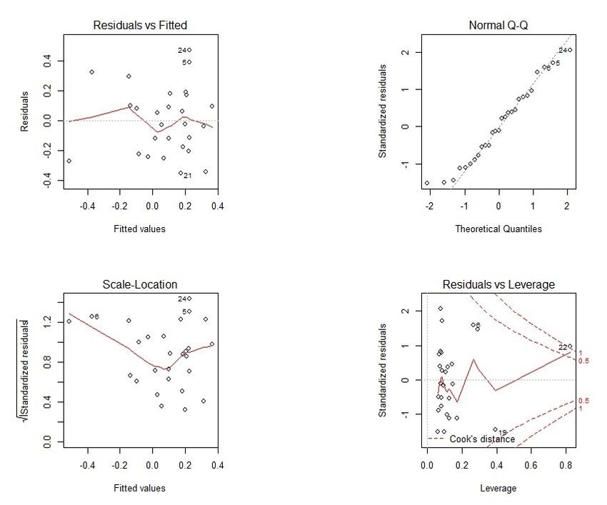
1    Introduction and Motivation
Brazil is the 5th largest country in the world with 8.5 million km2 and its population
in 2017 was 209,288.28 (The World Bank, 2018 and IBGE, 2018a). The Brazilian Gross
Domestic Product (GDP) is US$1.91 × 10¹² , making it the 9th highest GDP in the world,
according to the International Monetary Fund (2018a). However, the Brazilian GDP per
capita (considering Purchasing Power Parity), is US$16.11 thousand dollars annually, cor-
responding to the 84th higher position, much lower in the ranking (International Monetary
Fund, 2018b). The Human Development Index (HDI) is 0.759, see (UNDP, 2018a), which is
considered by the UN a High Human Development (HHD), since it is in the interval 0.7-0.8,
resulting in the 79th higher position in the World, according to the Human Development
Report from the United Nations Development Programme (UNDP, 2018b).
    The aforementioned figures may not reflect the entire country. Indeed, according to the
World Inequality Database (2015), the 1% richer has a national income share of 28.3% and
the bottom 50% share is only 13.9%. Considering income inequality Brazil is considered
the 9th most unequal country in the world (OXFAM Brasil, 2018). This leads us to
consider that indices and other metrics computed over averages should be considered as
inappropriate. In terms of people’s income, a special concern should be put on the data
distribution tail, particularly on the left tail.
    On the 2014 Edition of The State of Food Insecurity in the World, Brazil celebrated
its removal from the United Nations Hunger Map (Ministério do Desenvolvimento Social,
2014). The undernourishment rate in Brazil fell by half from 10.7% in 2000-02 to less than
5% in 2004-06. That report revealed that Brazil achieved both the Millennium Development
Goal (MDG), target of halving the proportion of its people suffering from hunger, and the
stricter World Food Summit (WFS) target of reducing by half the absolute number of
hungry people (FAO, 2014).
    In 2018, Brazil was at risk to go back to the UN Hunger Map (according to the General
Director of FAO - Food and Agriculture Organization (da Silva, 2018)). So, although
on average Brazil is considered to have a High Human Development, the uneven wealth
distribution makes that HHD is not a reality for its entire population. That leads to the
belief that the low-income people need extra protection. Besides, these particular people
live in risky, or riskier, environments and are more likely to be unable to cope with a crisis,
when compared to the “average people”.
    Our study object focus on a special micro pension programme inserted in the Brazilian
national social security system (managed by the INSS, Instituto Nacional de Segurança
Social, meaning National Social Security Institute). This special programme is called
Continuous Provision Benefit (CPB) and is a care benefit for low income citizens that did
not achieve the necessary criteria for getting the regular (public) pension. Controladoria-
Geral da União (2019) attests that this specific programme cost in 2018 less than 1% of
the total INSS expenditure.
    A citizen to be eligible for this benefit must prove that in his household the monthly
income per capita is less than a quarter of the Brazilian Minimum Wage, less than 2 Euros
per day, approximately, and must be either over 65 years old or disabled. Commonly, only
one member of the household receives this benefit, although there may be exceptions. This
programme can be considered as microinsurance in the sense of the protection of the low-
income people against specific perils and covers a variety of different risks, see Churchill

                                              2
(2006). In this definition, the word micro refers to the target market, instead of referring
to low premiums and low benefits. This is microinsurance from the government, a public
programme, it has a positive impact on the household of the eligible citizen and it truly
effects on the economy of some particular areas or cities in the country. For instance, we
underline that these applicant individuals can contribute up to 14 years and 11 months
before turning 65 or have contributed for a period of time before becoming disabled, but
if they do not reach the minimum requirements they do not receive the regular pension.
    This paper is a first study on the matter with this kind of dataset from Brazil, since
we work with the entire population of beneficiaries (4, 644, 698 people). Our study takes
place in a critical moment in Brazil when some changes are already happening, perhaps
significant, regarding social security in general, in which the micro programme is included.
Some changes are coming out publicly without any disclosure of a proper/rigorous study.
The data we work with here was provided to us in 2018, with the permission to analyse but
not to be disclosed. However, in the meantime the conditions regarding the data permission
have changed, and we feel there is now some uncertainty about future developments and
consultation study of the data.
    We work indeed with two different databases. The first with the entire population of
the programme and the second is a sample of the first with individualized information
like sex, date of birth, city of residence, UF (Federal Unit) of residence, start benefit date
and others. With the first database, we look at the programme from one angle, looking
for heterogeneity and how some economic factors impact differently in the applications
among all 27 Federal Units in Brazil. We are not looking for causality, but a good/proper
understanding. The main idea is to show the existence of clear inequalities among the
Brazilian Federal Units, which in turn may contribute to solving a serious problem. So,
besides looking for the impact of some economic variables, we want to see how they cluster.
These techniques are not particularly innovative nor highly sophisticated. However, we
found appropriate using fairly simple tools for our purpose.
    With the second database, we look at the programme from another angle. We aim
to analyse the impact of social protection for the elderly on the Brazilian National Social
Security System (INSS). To achieve this goal we separated the beneficiaries by UF and
by gender (since women and men have quite different life expectancies). Is this inequality
reflected on the “Expected Discounted Benefit” by beneficiary in the System (INSS)? Is
the system fair and, if not, can we make it more balanced?
    We focus on calculating the Expected Discounted Benefit of the protection for the
elderly. That is, we calculate a discounted value of future benefits, then we propose a way
to improve, or make the system fairer, for this we use Life Expectancy at 65 years old
and also at birth. We do so because on the former we need to compute how much the
government needs to estimate the amount reserved for this group, and the latter is due
to the inequality and heterogeneity among the Federal Units resulting in quite different
proportions of the population reaching the age of 65. To achieve a more homogeneous
system, we create two age adjusting factors for the programme that divide by UF and
gender and by UF, respectively.
    This paper is organized as follows. In Section 2 we do a short literature review, in
Section 3 we present our two databases and do descriptive analysis, in Section 4 we do
multiple regression modelling using Box-Cox and Yeo-Johnson models, and do appropriate
testing. In Section 5 we do cluster analysis. In the next section we compute the Expected

                                              3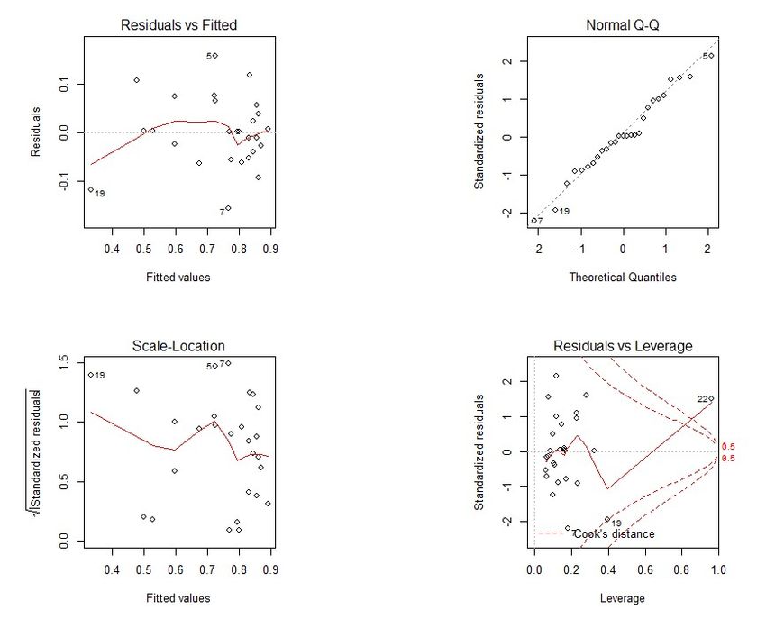
Discounted Benefit from our sample in the INSS and show how the system appears to be
unfair. In Section 7 we propose two Age Adjusting Factors (AAF) in order to achieve
a more equitable system. Afterwards, in Section 8 we exhibit a proposed reform for the
Brazilian Social Security and argue how it impacts the present and future beneficiaries of
this programme. Finally, we write some concluding remarks in Section 9.

2    Literature Review
In this section we talk about microinsurance in a broader sense, then about the Brazilian
social security system - INSS, and finally about the intersection between these two: Mi-
croinsurance in the INSS, denoted as “Continuous Provision Benefit” (directly translated
from the Portuguese Benefı́cio de Provisão Continuada). Our study is focusing on this
intersection. Figure 1 gives a quick picture of how specific microinsurance interacts with
the public pension system in Brazil.

            Figure 1: Intersection between Social Security and Microinsurance

    As defined in the Introduction, microinsurance is the protection of low-income people
(Churchill, 2006, a reference book on the matter). Poor households often have informal
means to manage risks, but informal coping strategies generally provide insufficient pro-
tection. Also, Jacquier et al. (2016) say that

          Microinsurance schemes may assume some social protection functions, such
      as redistribution through internal cross-subsidies or by channelling public sub-
      sidies to their members.

    From the INSS (2019) we quote (our translation)

          The INSS was created on the 27th of June 1990, through Decree No. 99,350,
      as a result of the merger of the Institute of Financial Administration of Social
      Security and Assistance (Instituto de Administração Financeira da Previdência
      e Assistência Social, IAPAS) with the National Institute of Social Security
      (Instituto Nacional de Previdência Social - INPS), as an autarchy linked to the
      Ministry of Social Security and Social Assistance (Ministério da Previdência e
      Assistência Social, MPAS).
          ...
          The INSS is responsible for the operationalization of the recognition of the
      rights of the insured individuals of the General Social Security System (RGPS),

                                             4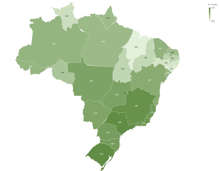
covering more than 50 million policyholders and having approximately 33 mil-
     lion beneficiaries in 2017.
         ...
         Article 201 of the Brazilian Federal Constitution observes the organization
     of RGPS as a contributory and compulsory affiliation, where all the INSS’s
     activities fit in, respecting government policies and strategies from hierarchi-
     cally superior bodies, such as ministries. The entity is currently linked to the
     Ministry of the Economy.

     Deblon and Loewe (2012) say that although vulnerability and poverty are not the
same, poor people are more vulnerable because they are exposed to a higher number of
risks. Therefore, these two reinforce each other. There is a vicious circle: The occurrence of
risk decreases people’s well-being, it may force them to use their financial and social assets
to cope with the effects of such risk, but the vulnerability reduces the ability to extend
their economic activities and improve their socio-economic well-being. Social protection is
the total set of actions that are carried out by the State or other players to address risk,
vulnerability or chronic poverty. In this paper we focus in the State as a player. Social
security consider typical risks for people who derive their income from paid labour, i.e., for
low-income people. Its goal is to break this vicious circle.
     Microinsurance is not a substitute for a social transfer scheme because microinsurance
addresses vulnerability rather than chronic poverty, while social transfers provide imme-
diate support to people in poverty. If properly designed, microinsurance constitutes an
efficient means of providing individuals in need with social safeguards. In this way, it can
potentially contribute to closing existing gaps in coverage with the usual social protection
schemes operating in developing countries. There are, however, some limitations to the
potential of microinsurance (Deblon and Loewe, 2012).
     Apart from Brazil, there are other examples of implementation of programmes of mi-
croinsurance for social protection in developing countries, see for instance, Arun and Steiner
(2008). They outline the status of microinsurance provision in Ghana and Sri Lanka. Roth
et al. (2007) attest that the percentage covered by microinsurance in Asia is 2.7 percent, in
Africa is 0.3 and in Latin America is 7.8. We restrict our analysis to this sort of microin-
surance programme in Brazil, and covers over 4.5 million people. Unlike other authors we
do a technical and quantitative analysis only.
     The Continuous Provision Benefit (CPB) of the Organic Law of Social Assistance
(LOAS) guarantees a minimum (monthly) wage paid for 12 months (it does not include the
traditional 13th salary) for the disabled and for the elderly, 65 years of age or older, who
prove not having enough means to provide their own maintenance, or even from his family.
It is indeed a micro pension programme. Brazilians or Portuguese residing in Brazil can
apply to this benefit.

3    The Data and descriptive analysis
Quantitative Information for our study is not easily available, exploring it is pioneering
research. Our data was provided by the Superintendence of the INSS. We realized an
existing gap in the literature about this particular subject, we do value the importance of
using and analysing this data. As we said in the Introduction, we have two different sets

                                              5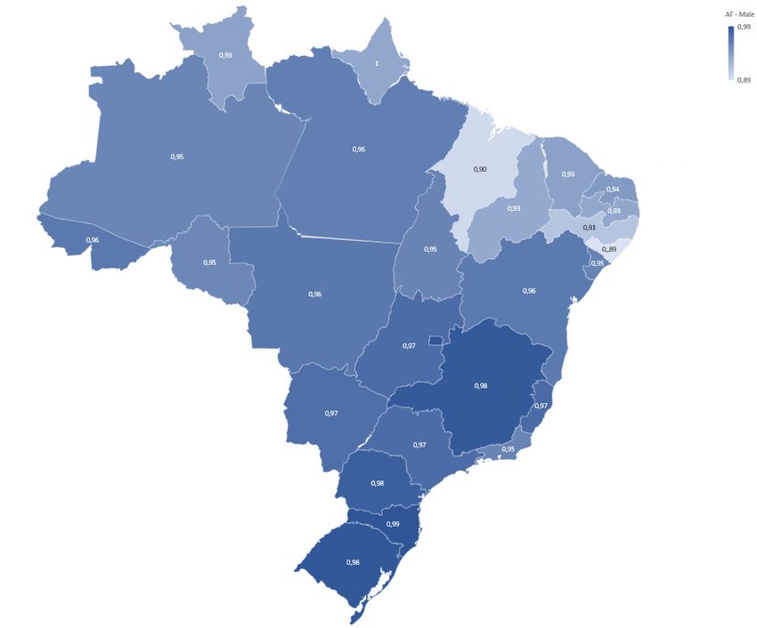
of data that we are now presenting. The first one consists on the entire population of the
programme under study. However this population is only divided by UF and not by gender.
On the second database we will present a sample of the population with information on
every individual. We will use the first database on Sections 4 and 5 and the second on
Sections 6 and 7.

3.1   The First Database
The data consists on all the Brazilian citizens (and Portuguese) that receive this specific
benefit, the CPB. We also separate the beneficiaries that belong to the group aforemen-
tioned, that is, people that receive the benefit called Amparo Social ao Idoso and Amparo
Social Pessoa Portadora de Deficiência, which means “Social Support to the Elderly” and
“Social Support for Disable Person”, respectively, literally translated. The total group is
4,644,698, from these 2,595,775 are disabled and 2,048,923 elderlies, corresponding to 56%
and 44% respectively.
    Brazil has 27 Federal Units (UF) consisting on 26 states plus the Federal District (the
capital district). We refer to Table 3 in Appendix A where we can see for each UF, names,
codes and the different life expectancies that are used throughout this work.

                                 Figure 2: Total bnf (%)

                                            6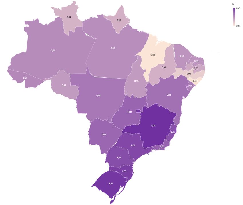
Figure 3: Elderly bnf (%)

Figure 4: Disabled bnf (%)

            7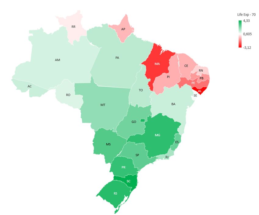
Figure 5: Population by UF

    The number of beneficiaries vary significantly by UF, but we can not compare this
nominal numbers since the UF’s can have quite different population sizes. Since each state
population vary from 450,479 to 41,262,199, we found necessary to divide the number of
beneficiaries (bnf) by the population size so we can compare ratios from each UF. Figures 2-
4 show the number of beneficiaries by UF, for total, elderly and disabled, respectively.
Figure 5 refers to the population size.
    Figure 2 is in descending order by ratio, the following two keep this same order to
enhance the position change amongst them. It reveals some interesting points that are
worth mentioning, for instance, Pernambuco is a state that although is the 5th in the
Total ranking, when we consider only Disabled, calls our attention. One of the reasons
for this deals with a health problem that occurred in Brazil, Pernambuco was particularly
affected (microcephaly, 2015).
    In Figure 6 we present three boxplots that show the distribution of the ratios afore-
mentioned.

   Figure 6: Ratios of the number of people in Social Support and the UF Population

                                             8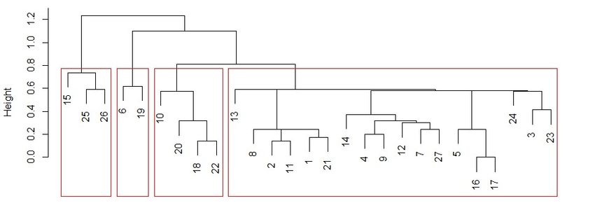
When analysing Figure 6, the first aspect to mention about the shape of the data
distribution is that the ratio of the Total and Disabled has a positive asymmetry and the
Elderly has a reversed one. Also, the ratio for the Elderly varies from 0.42 to 1.92 while
the ratio for the Disabled varies from 0.83 to 2.6, which shows that not only the Elderly is
more concentrated but also the scale is lower.
    From these boxplots we can observe that the Elderly group is the one with more promi-
nent outliers. These outliers correspond to Numbers 5, 19 and 24 representing Mato Grosso
do Sul, Santa Catarina and Amapá respectively. Both Mato Grosso do Sul and Amapá
have a lower population density when compared to other states. Mato Grosso do Sul is
located in the Center-West region, has a density of 6.86 per km2 . When we consider the
economic variables we analyse, this state does not outstand, indeed it has the 7th highest
monthly nominal income per capita, R$ 1, 291.00, and the real average income in (formal)
employment is R$ 2, 361.00, corresponding to the 10th position.
    Amapá is located in the North region with a density of 4.69 per km2 , has the second
lowest population size among all states, only 669.526 (in 2010 census, IBGE, 2018b) and
an estimated population for 2018 of 829.494 people (IBGE, 2018a). Although it has the
highest ratio for Elderly that are considered poor and receives a benefit, the real average
income of people in formal employment is R$ 3, 131.00, which is the second highest average
income among the states.
    An interesting outlier in this is Santa Catarina, that is located in the South region,
because this state has the lowest (by far) Elderly receiving benefits and Population ratio,
but it has the highest life expectancy (79.1). Santa Catarina doesn’t have the highest
neither HDI nor income per capita but manages to have the lowest ratio.

3.2   The Second Database
The sample that is analysed consisting on citizens that started receiving a pension or
a benefit from the INSS in the period from 02/01/2018 until 06/04/2018. We selected
the beneficiaries that belong to the group aforementioned, that is, people that receive
the benefit called “Amparo Social ao Idoso” and “Amparo Social à Pessoa Portadora
de Deficiência”, which means “Social Support for the Elderly” and “Social Support for
Disable Person”, respectively. The total pensioners or beneficiaries of the system consists
of 1,332,080. People that received this particular benefit are 81,840, being 40,372 elderlies
and 41,468 disabled.
    In Table 1 we show a short description of the distribution of the age at grant of benefit
for all beneficiaries in the programme in our sample: Minimum, 1st to 3rd Quartiles,
Maximum and Mean, denoted as M in, Q1-Q3, M ax and M ean, respectively. We removed
from the elderly and the disabled group those people who are entitled to the benefit as
survivors of previous beneficiaries. We ended up with 40,227 elderlies and 41,387 disabled
entries. We note also that often the benefit is granted after the age of 65 due to a delay in
the application process.
    In Figure 7 we present graphs of the distribution of beneficiaries by sex. The first plot
corresponds to the Elderly, from those 57% are women. In the case of the disabled we
have 56% male and among total beneficiaries of CPB of our sample we have 50% each,
approximately. This is probably due to a higher male mortality rate and disability rate.
Although in total the distribution looks well balanced, it is not the case when we separate

                                             9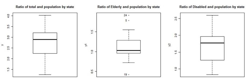
Variable     M in    Q1   M edian    M ean    Q3       M ax
                 Disabled      0       9     33       31.45    52        81
                 Elderly       65     65     65       66.46    67       106
                 Total         0      33     64       48.71    65       106

    Table 1: Distribution of age at grant of benefit (data period: 02/01-06/04/2018)

                       Figure 7: Distribution of beneficiaries by sex

Elderlies and Disabled, where there is a clear gender difference.
   We have available official figures for Life Expectancies by Federal Unit, as well as by
gender, for the entire population and we will try to adjust the benefits according to age.
These Life Expectancies are displayed in Appendix A. Since the disabled group does not
have a minimum age and there is no official Life Expectancy for the disabled population
subset, in what follows we devote our efforts on the Elderly Group only.

4    Modelling Social Support using Multiple Regression
In this section we aim to study how economic factors can explain the quantity of peo-
ple receiving the social support of the microinsurance programme in Brazil. Radermacher
et al. (2012) state that impact evaluations for microinsurance are often complicated, expen-
sive and sometimes difficult to implement. Therefore, less robust techniques predominate.
Among the robust approaches are those that use statistical or econometric techniques.
They also suggest in particular a regression analysis to take into account of mitigating

                                            10
factors such as income, race or gender. Following these ideas we use income as mitigating
factor but not separating people regarding race or gender. Our quantitative study use
regression models where explanatory variables explain the effect by UF/state.
We chose three different response variables to check whether we find different impacts
on them. These three variables are: Total of Social Support, Social Support for the Elderly
and Social Support for the Disabled. For each response variable we have 27 entries (UF’s).
The explanatory variables are: HDI (according to the UNDP (2018c)), Nominal Monthly
Income per capita (according to the Ministry of Labour, RAIS), Life Expectancy at birth
and Demographic Density (IBGE (2018b) and IBGE et al. (2018)). Since the requirements
to acquire the benefits do not distinguish gender, on the regression model we cannot select
groups accordingly.
In order to analyse the number of beneficiaries by UF, we consider the above four
economic variables, and with these we have set four studying hypotheses, labeled H1-H4:
H1 We are studying a microinsurance programme, so we start by considering that to an
UF with a higher Human Development Index should correspond to a lower ratio on
people in need of this programme;
H2 The main condition to acquire this benefit is to have an income of less than a quarter
of the Brazilian minimum monthly wage. So, one of the variables that we use is the
Nominal Monthly Income per capita, under the hypothesis that UF’s with a higher
nominal monthly income per capita should correspond to a lower ratio of beneficiaries;
H3 Since a person that acquires this benefit will receive it until death, our third hypoth-
esis is that Federal Units with higher Life Expectancy should result in a higher ratio
of beneficiaries. We are going to check if this is replicated on our population;
H4 Areas that have a higher Demographic Density also present more poverty [see Szwar-
cwald et al., 1999 next], so our last hypothesis is that the Federal Units with higher
demographic density should also correspond to a higher ratio.
Szwarcwald et al. (1999) show that the income inequality affects the homicide rates and
this was found precisely in the part of the city with the highest concentration of slum
residents (demographic density). In Brazil the following three factors go hand to hand: 1.
Income inequality; 2. Demographic density; and 3. More violence which leads to a decrease
in Life Expectancy.
Bourguignon and Chakravarty (2003) attests that poverty is a multidimensional concept
and that to a person to be considered poor it is necessary to fall below at least one of various
lines. When applying this concept to Brazil, they define poverty according to income and
education. The authors also say that this concept goes in the same direction as the Human
Development Index that aggregates per capita real GDP, Life Expectancy and Educational
Attainment Rate. For this reason, we consider that once more the income monthly per
capita and Human Development Index are important variables to be taken.
Two years later, Thorbecke (2005) said that authors when trying to measure multi-
dimensional poverty only deal with a maximum of four factors and usually use only two.
In this paper we used four different factors. Thorbecke (2005) also said that the standard
way of assessing whether a person is under or above the poverty line is his income and this
11AIC BIC
Total Elderly Disabled Total Elderly Disabled
Linear X X -54.2 X X 29.60384
Quadratic -46.63 -66.68 -64.63 39.77159 18.4178 21.76626
Box-Cox -108.96 -73.71 X -22.56316 11.39623 X
Yeo-Johnson -133.04 -72.92 X -46.63863 12.1794 X
Table 2: Model selection
is a limited perspective. In this paper we try to see if the four aforementioned factors are
also statistically significant for the ratio of beneficiaries of this micro programme.
More recently, Golgher (2016) also talks about multidimensional poverty in Brazil. The
author talks about deprivation in households and how some types of deprivation, as food,
specially affected the low-income ones. And then how to differentiate medium-income from
higher income households from the deprivation of education and some non-popular goods,
respectively. In this paper we focus on the low-income households, on those people that
are deprived of food, the most basic and important need.
To select a model, we use the four different approaches: 1. Linear; 2. Quadratic (allow-
ing the explanatory variables to be quadratic); 3. Box-Cox transform; and 4. Yeo-Johnson
transform (both are transformations on the response variable). We take as selection crite-
ria AIC and BIC (Aikaike and Bayesian Information Criteria, respectively). If both give
a similar result we keep the simplest. At first, the models were selected so that all the
included variables and the model itself were statistically significant, so we started with 12
models. Then, we set a first filter that is the Ramsey Regression Equation Specification
Error Test - Reset Test (Ramsey, 1969). We were left with eight models. Throughout the
paper we used a significance level of 10%. Table 2 presents the AIC and BIC for the mod-
els, those which failed the Reset Test are represented with an “X” and the chosen models
are written in bold. Both criteria lead us to the same conclusion: The model for the Total
of beneficiaries is the one with the Yeo-Johnson transform for the response variable. For
the Elderly, it is the one with the Box-Cox transform and for the Disabled is the one with
no transform on the response variable. All of them are allowing the explanatory variables
to be quadratic.
The estimated model for the Total group is shown below:
Yyj = −8.623 × 10 − 8.41 × 10−4 X2 + 2.372X3 + 2.942 × 10−7 X22 − 1.605 × 10−2 X32 ,
where Yyj is the Yeo-Johnson transform of Y (ratio of people by state that receive Social
Support), X2 is the Nominal Monthly Income per capita and X3 is the Life Expectancy
at Birth. This model shows a Determination Coefficient - R2 of 0.8007 that means that it
explains about 80% of the reality that represents, the highest from the three select models
(the Adjusted Determination Coefficient, Ra2 , is 0.7644).
Then, we performed the Bera-Jarque test to check normality in the residuals (Jarque
and Bera, 1980), the p-value was 0.9797, resulting in not rejecting a Normal distribution.
To test linearity we used the Rainbow test (Utts, 1982), in this case the p-value is 0.1802.
12Figure 8: Ratio: Total bnf / Population by UF
So, we do not reject linearity. To detect heteroskedasticity, we used the Koenker test
(Koenker, 1981), and we did not reject homoscedasticity, we got a p-value of 0.442. With
respect to multicollinearity, for all three cases using Variance Inflation Factor, we observed
multicollinearity, but when checking the correlation between the explanatory variables, the
only ones that were high were those between X2 with X22 and X3 with X32 , which was
already expected and we did not considered it a problem.
In Figure 34 in the Appendix, we present four plots, the first is residuals versus fitted
values where we do not see any pattern in the residuals. The second one is the Normal
Q-Q plot where we can see three outliers, UF’s 5, 7 and 19. The third one shows the
Scale-Location and the fourth Residuals versus Leverage.
In this model we have four outliers, 5, 7, 8, 19, 22 that represent the following feder-
ative units: Mato Grosso do Sul, Goiás, Maranhão, Santa Catarina and Distrito Federal,
respectively. From those, Santa Catarina and Distrito Federal are influential points and
8, 19 and 22 are high-leverage points (using influence measures).
Figure 8 show Brazilian map to highlight the UF’s that are outliers. The scale represent
the range of the ratio, the darker color represent higher values.
Figure 9 and 10 present the impact from X2 and X3 on the response variable, the ratio
between total bnf and population size.
13Figure 9: Nominal monthly income on YY J Figure 10: Expectation of life on YY J
We can see that both variables have a linear and a quadratic component. It results
on a curved line. In Figure 9 we can see a smile shape while in Figure 10 we see the sad
shape.
The nominal monthly income per capita varies from R$ 597 to R$ 2, 548. Until turning
point R$ 1, 429 it decreases the ratio of total beneficiaries by UF. After that it starts to
increase, however throughout the range of income pc has always a negative impact. Life
Expectancy at birth has the opposite behaviour. Increases the ratio until 73.9 years old
and after this turning point it starts to decrease. Also, inside the range the impact is
always positive.
Focusing now on the Elderly group, Y 1 is now the response variable to the ratio of
people by state that receives the Social Support for the Elderly we have to following
estimated model:
Y 1bc = −1.780 × 10² + 4.837X3 + 1.403 × 10−7 X22 − 3.284 × 10−2 X32 ,
where Y 1bc is the Box-Cox transform of Y 1, X2 is the Nominal Monthly Income per capita
and X3 is the Life Expectancy at birth.
This second model gives an R2 of 0.4557, the lowest from all three selected models, it
explains almost half of the analysed data. The Adjusted Determination Coefficient, Ra2 ,
has a value of 0.3847. The Bera-Jarque test has p-value of 0.6052, and the Normality was
not rejected. The Rainbow test has a p-value equal to 0.259, so, we do not reject linearity.
With respect to the Koenker test we also did not reject the null hypothesis (p-value of
0.727).
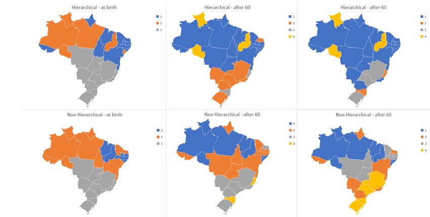
Figure 35 present similar plots to those in Figure 34 regarding the second model.
As we can see from Figure 35, this model presents six outliers, 5, 6, 19, 21, 22 and 24
that represent the following UF’s: Mato Grosso do Sul, Espı́rito Santo, Santa Catarina,
Sergipe, Distrito Federal and Amapá, respectively. The high influential points are Espı́rito
Santo, Santa Catarina and Distrito Federal and Distrito Federal is a high-leverage point.
In Figure 11 we show the map with Y 1, the ratio for the Elderly. Figures 12 and 13
present the impact of X2 and X3 in Y 1bc .
14Figure 11: Ratio: Elderly bnf / Population by UF
Figure 12: Nominal monthly income on Y 1BC Figure 13: Expectation of life on Y 1BC
Regarding this model, the variable X2 has only a quadratic component, and X3 has
both linear and quadratic. For the entire range, the Nominal Monthly Income per capita
increases the ratio of the Elderly bnf by UF. Also, this component is always positive. The
Life Expectancy at birth has a different behaviour. It takes the ratio to increase until 73.6
years old and after this turning point it starts decreasing. Also, inside the range of Life
Expectancy, the impact is always positive.
Y 2 represents the response variable to the number of people by UF that receive the
15Social Support for Disability we have to following estimated model:
Y 2 = −1.445 × 10² − 3.368 × 10−3 X2 + 4.003X3 + 1.018 × 10−6 X22 − 2.696 × 10−2 X32 ,
where Y 2 is the Ratio for Disabled, X2 is the Nominal Monthly Income per capita and X3
is the Life Expectancy at birth.
At last, on this model the R2 is equal to 0.7207. The Ra2 has a value of 0.6699. In
this case, similar to the others, both tests did not reject the null hypothesis (p-values were
0.7397 and 0.2524) for the Bera-Jarque test and the Rainbow test, respectively. The same
happened with the test to determine if our variance was heteroskedastic. With a p-value
of 0.257, we do not reject the homoscedasticity hypothesis.
Figure 36 presents the four plots regarding the model as aforementioned.
On this model, we can observe that 1, 6, 8, 11, 16, 19, 22, 23 and 26 are outliers, they
represent Alagoas, Maranhão, Pará, Rio de Janeiro, Distrito Federal, Acre and Roraima,
respectively. The high influential points are Maranhão, Distrito Federal and Roraima and
the high leverage points are Espı́rito Santo, Santa Catarina and Distrito Federal.
Figure 14 displays the Brazilian map using the ratio for Disabled as scale, also to
highlight the outliers UF’s.
Figure 14: Ratio: Disabled bnf / Population by UF
Figures 15 and 16 exhibit the impact of both explanatory variables on the ratio. In this
model the impact has a similar behaviour as the variables in the first model, considering
the Total group.
16Figure 15: Nominal monthly income on Y 2 Figure 16: Expectation of life on Y 2
We can observe in Figures 15 and 16 that both variables have a linear and a quadratic
component. Until R$ 1, 654, the Nominal Monthly Income per capita decrease the ratio
of total beneficiaries by UF. After that turning point, starts to increase. Throughout the
range of Income per capita the impact is always negative. The Life Expectancy at birth
has the same behaviour for all three models: Increases the ratio until a turning point and
then decreases, in this case the turning point is 74.24 years (the oldest from all models).
Also, inside the range of Life Expectancy the impact is always positive.
Some interesting remarks are that although HDI among UFs vary from 0.63 to 0.82,
HDI was not statistically significant in any of the chosen models. The same happened to
Demographic density, that varies from 2.01 to 444.66 and was not significant either. The
UF number 22, that represents the DF, was an outlier on all three models. The Nominal
Monthly Income per capita has a different impact on the models. The Life Expectancy at
birth has a similar behavior, changing only at the age of the turning point: 73.9, 73.6 and
74.24, respectively.
When we defined the models, in the beginning of Section 4, we had four hypotheses.
In all three models the variables HDI and Demographic Density were not statistically
significant, for this reason we can not neither accept nor reject any H1 and H4.
Regarding H2, we were testing whether the increase in Nominal Monthly Income per
capita would decrease the ratio of beneficiaries. On the Total and Disabled models this
happens when we start to increase the Nominal Monthly Income, however after the turning
point (R$ 1, 429 and R$ 1, 654, respectively) it increases and in the case of the Elderly model
the ratio increases for the entire range. Therefore, we reject H2.
Finally, concerning H3, we expected to see an increase in ratio when we had an increase
in Life Expectancy in the UF’s. In all three cases this is what happens in the beginning,
however it is not linear, it is quadratic, which means that after the turning point starts to
decrease. So, we do not completely reject our hypothesis. Instead, we change it.
These results are very interesting due to the fact that they show that you do not capture
the heterogeneity among the UF’s, in such a way that you could just either increase or
decrease one variable and adjust the ratio of beneficiaries. Also, the UF’s have similar
behaviour, that is, we observed a geographic pattern among UF’s, which lead us to look
for clusters. We do that in the section that follows.
175 Cluster Analysis
Cluster analysis is a group of multivariate techniques whose primary purpose is to group
objects based on the characteristics they possess (Hair Jr. et al., 2014). It aims to explore
data sets to assess whether they can be summarised in terms of a limited number of groups
of individuals with some sort of similarities and which are different in some respects from
individuals in other clusters (Everitt et al., 2011).
After observing the results in the previous section, we decided to look for clusters, more
specifically, if we could have some geographical groups. We analysed hierarchical and non-
hierarchical clusters, separately. We performed an analysis based on three different Life
Expectancies: At birth, at 60 and 65 years old. Our motivation lies in looking in which
cases the Life Expectancy would be lower but because of young people dying (usually as a
result of violence).
A hierarchical clustering method produces a classification in which small clusters of very
similar observations are nested within larger clusters of less closely-related observations. In
a hierarchical classification the data are not partitioned into a particular number of classes
or clusters at a single step. Instead, the classification consists of a series of partitions, which
may run from a single cluster containing all individuals, to having a single individual per
cluster (Everitt et al., 2011).
We used the Euclidean distance measure to compute the distance matrix and the single
method for the cluster agglomeration. The hierarchical clustering process can be portrayed
graphically in several ways. Firstly we present dendrograms. That is a common approach,
which represents the clustering process in a treelike graph (Hair Jr. et al., 2014).
Figure 17: Dendrogram for the expectancy of life at birth
From the dendrograms we can observe that UF’s numbers 21, 2 and 11 that represent
Sergipe, Amazonas and Pará are the farthest left and in a cluster with 15, 25, 26 that
represent Piaui, Rondônia and Roraima. In Figures 18 and 19 these three (15, 25, 26)
are those in the extreme left, while (2, 11 and 21) are in the middle of the dendrogram.
Another fact is that on Figure 19 we have a much flatter dendrogram and one of the clusters
comprehends 18 out of 27 UF’s.
In Figure 17, Espı́rito Santo and Santa Catarina (6, 19) are amongst the others, in
the biggest cluster. On the regression models these two were outliers, this is shown on
the clustering using the Life Expectancy for a person that reaches 60 and 65 years old,
18Figure 18: Dendrogram for the expectancy of life for the person that is 60 years old
Figure 19: Dendrogram for the expectancy of life for the person that is 65 years old
respectively. In both cases the two UF’s are excluded from the others in a cluster that only
contains them.
We can observe in the maps in Figure 33 the three UF’s are clustered together and this
cluster consists on people that got to 60 and 65, but present a lower expectancy. These
three UF’s are Piauı́ in the North-East region and Rondônia and Roraima from the North
region. From these maps we can see a high geographic correlation on the homogeneity
amongst the clusters.
In contrast to the hierarchical methods, non-hierarchical procedures do not involve the
treelike construction process. Instead, they assign objects into clusters once the number
of clusters is specified (Hair Jr. et al., 2014). The non hierarchical clustering algorithms
are used mainly for extracting compact clusters by using global knowledge about the data
structure (Dzwinel et al., 2004).
In the case of people that are 60 years old, the UF’s 6 and 19 are in a separated cluster
both in the hierarchical and non-hierarchical analysis. Rio Grande do Norte is the only UF
from the upper part to be clustered (in grey) with the UF’s from the lower part of Brazil.
On the Life Expectancy at birth, regions South, Center West and South East constitute
one sole cluster, both when clustering hierarchically or non hierarchically. The highest
difference between these two structures is in the third case, people that are 65 years old.
When you consider people that already lived until 65, in the South-East region Rio de
Janeiro is clustered along with states from the upper part in Brazil. This happens in the
19hierarchical and non hierarchical cases.
We showed the existence of high heterogeneity, for some chosen economic variables,
on the population of beneficiaries among Federal Units (UF’s), specially among the five
regions in Brazil (North, North-east, Centre-west, South-east and South), which has an
obvious impact on the beneficiaries of the programme.
Next we go much further, using a different database, we want at first to calculate
the amount that INSS spends with the beneficiaries, estimate values per capita, then the
weight of each UF and see if this high heterogeneity is also reflected on the benefit amounts.
For the estimate calculation, we use a more comprehensive database that includes every
Brazilian that started receiving a pension or a benefit from the INSS in the period from
2nd of January 2018 to 6th of April 2018. Using this database we focus on the beneficiaries
of this specific programme. In the first database we had the same population but with
fewer information and in this second despite only using a sample of data, we have more
specific information on every individual.
6 Expected Discounted Benefit
In this section we calculate an estimate of the Expected Discounted Benefit (briefly, EDB)
for the beneficiaries of our sample in the elderly group. It is indeed an estimate of the
expected present value of the future monthly benefits, at some discount rate. As aforemen-
tioned (end of previous section) we use the Life Expectancy for an individual that is already
65 years old, since this is one of the criteria to be eligible for the programme. We chose
an annual discount rate of 6%, this is the official return rate for Brazilian treasure bonds
in 2019. Since the benefit is a monthly payment we use the equivalent monthly rate of
0.486755%. It is clear that there is a greater heterogeneity on life expectancies among UF’s
as well as between genders. Since the poorer states have a lower LE, it is clear that most
beneficiaries of the programme live in the wealthier states, despite the fact that it can be
argued that most of public money come from those richer. Although, we could counteract
that public social policies should target the poorer regions. Knowing this, we can pose the
following question: Is there a way to narrow differences among these sub groups? We can
do changes on benefits (often not well viewed) or, better, change retirement ages without
doing any changes to the benefits. Both approaches have pros and cons, we will come to
this later. We observe for instance that in some poorer UF’s life expectancies are much
lower, much lower in some cases, resulting in many people not taking the benefit where it
would be needed more, in the sense that there are poorer people, relatively speaking. Our
starting tool is the calculation of the Expected Discounted Benefit.
To explain the calculation technique used let’s put some mathematics, although simple.
First define locally some quantities, in order to set clear the calculation of the necessary Age
Adjusting Factors (briefly AAF). We show the calculation separating by gender, although
the second proposal does not separate but calculation method is likewise.
Let b be the minimum monthly wage which equals the monthly benefit. Let C(i, j, k, l)
be an estimate for the present value of the benefit cost by UF i, sex j, in time k, for
individual l. The variable time here is measured in months after some reference age.
For simplification we consider that if a beneficiary does not live a full month the benefit
is not paid, benefits are paid at the end of each month (to be precise in our case it is
20on the 28th or 29th). Let r be the monthly equivalent discount rate. Here we have
r = 0.00486755 ' (1.06)(1/12) − 1. Also, let ni be the number of beneficiaries in UF i,
LEij is the Life Expectancy in UF i for sex j (i = 1, . . . , 27, j = 1, 2). It’s clear we are
using 54 Life Expectancies. Define LTlij as the Expected Lifetime of individual l in UF i
for sex j, in exceeding months after a reference date, we use the date of 06/04/2018, the
last day of granting benefit in our sample. This way we garantee that all individuals in
our sample are already receiving a benefit. For instance, if Life Expectancy is 69 exactly
for some for individual l in state i and sex j, withP granting age 65 years and 2 months (in
06/04/2018), then LTlij = 46 months. Let n = 27 i=1 = nj = 40, 372 be the number of
beneficiaries in our sample. In another way, let’s consider also ni = mi1 + mi2 , separating
by gender (subscript 1 stands for male, female otherwise), where mij is the number of
people of sex j P
in UF i, i = 1, 2, . . . , 27 and j = 1, 2. Following a similar notation reasoning
27
we set mj = i=1 mij as the number of people of sex j in the whole country. Then
n = m1 + m2 = 17, 351 + 23, 021 = 40, 372, by order male and female.
In our sample, for individual m from UF i with sex j, we have that
b
C(i, j, k, l) =
(1 + r)k
LTlij
X b
C(i, j, l) = = b aLTlij r
(1 + r)k
k=1
ni
X
C(i, j) = C(i, j, l) .
l=1
It is clear that C(i, j, l) is the present value of all benefits received by individual l until LTlij ,
and C(i, j) is the present value of all benefits in UF i for sex j. an r is the standard formula
of the temporary unit payment, with term n and discount rate r, financial annuity. For
simplification we consider that every individual is receiving in 6/4/2018 the full amount of
the monthly benefit. We use the LTlij for all individuals of UF i, it is a clear simplification
because there are no mortality tables available for each UF, only the national ones.
Then for the whole of Brazil, we have
27
X
C(j) = C(i, j)
i=1
2
X
C = C(j) .
j=1
The Expected Discounted Benefit for the our sample is e 1, 105, 411, 797.02. When
considering Life Expectancy at birth the value estimate equals e714, 044, 109.82, this big
difference is brought by the LE’s. The real amount that the INSS will spend with the
beneficiaries in our sample is a value between these two and closer to the first one. We
used the exchange rate from the day 04/04/2019, making e1 corresponding to R$ 4.35,
therefore we have for Life Expectancy at 65 and at birth the amounts R$ 4, 808, 541, 317.02
and R$ 3, 106, 091, 877.73, respectively. From now on all values are shown in Euros.
We are interested in calculating the necessary Expected Discounted Benefit for a bene-
ficiary in the programme, that starts receiving the benefit now. From this amount we could
21estimate the necessary amount for the entire population of beneficiaries. However, we do
not require this latter value to achieve our goal, due to the fact that we want to analyse the
Expected Discounted Benefit estimate per capita by UF, looking for heterogeneity among
UF’s.
Figure 20 shows in blue bars the amount corresponding to the Expected Discounted
Benefit by UF (absolute values), while in orange we show the cumulative amount (in
%). Under the bars are the corresponding names of the UF’s. We can draw attention
to São Paulo (it is the wealthiest UF) that corresponds to 23.61% of the total amount
while Roraima (the UF with smallest population and the lowest GDP) measures up to
only 0.19%. We also need to take into consideration the fact that the population of these
UF’s is of 41,262,199 and 450,479 people, being the most and the least populated Federal
Units in Brazil respectively. Therefore, obviously we can not use the Expected Discounted
Benefit by itself, so we will consider the Expected Discounted Benefit per capita. We can
already spot heterogeneity among UF’s.
Figure 20: Expected Discounted Benefit (EDB) by UF’s in Euros
In Figures 21 and 22 we present the distribution of Expected Discounted Benefit sep-
arating by sex. It is important to highlight two facts. The first is that there is a huge
difference between genders. In Figure 21 we can observe that when we consider LE at birth,
the male beneficiaries represent only 27% and when considering LE at 65 it represents 40%.
This is due to the fact that in Brazil there is a large disparity in Life Expectancy between
genders. For instance, in the UF Ceará this disparity is of 8.28 years on LE at birth. The
disparity varies from 4.99 to 8.28 with an average of 6.8 years for LE at birth. For LE at
65 it varies from 1.9 to 4 and the average is 3.03. That is why on the case of LE at 65
the female group represents 60% of total, it portrays the decrease of the difference between
genders.
The second fact is the disparity that we can observe from Figure 22 between the Ex-
pected Discounted Benefit calculated with different Life Expectancies. The reason for this
is the fact that in Brazil a significant part of the population dies before 65.
We aim to analyse the Expected Discounted Benefit by Federal Unit and subsequently
22Figure 21: Expected Discounted Benefit (EDB) in Euros: LE at Birth and at 65
Figure 22: Expected Discounted Benefit (EDB) in Euros: LE at Birth and at 65
try to make the system more homogeneous. Not rejecting alternatives, a simple but ef-
fective method we propose is creating a kind of actuarial correcting factor to take into
consideration the Life Expectancy disparities among Federal Units. We also separate by
gender in one of the proposals. This is done in a way that considers that every beneficiary
in Brazil presents the same Expected Discounted Benefit estimate. Although we considered
the LE at 65 to see how much the government will spend by UF, for the purpose of policy
making we will consider LE at birth only. This is because we need to take into account
that there are UF’s where a greater part of the population will not reach 65. This coincides
with the poorer UF’s, those were the UF’s that were supposed to need more support from
this programme.
Figures 23-25 show the Expected Discounted Benefit per capita, first for the male group,
then the female group and finally the total. On these figures we will represent inside the
red frame is the average of the beneficiaries in our sample, Brazilian’s average estimate.
In Figure 23 we exhibit the EDB by UF in descending order of amount. Amounts vary
23Figure 23: Expected Discounted Benefit (EDB) - Male Group
from e2, 340.64 to e15, 284.70, so we can clearly spot the heterogeneity among UF’s, with
the exception of the UF Rio de Janeiro, marked green, Acre (North) and Bahia (Northeast),
the UF’s above the average are from the regions: South, Southeast and Centre-West and
those below the average are from the North and Northeast region.
In the case of the female group, we can observe in Figure 24 that the UF that presents
the lowest Expected Discounted Benefit per capita is Maranhão, with the amount of
e16, 600.42. This figure is already higher than the highest Expected Discounted Bene-
fit per capita from the male group, that was Santa Catarina, with e15, 284.70. Therefore,
there is no intersection between these two intervals, being the latter from e16, 600.42 to
e25, 211.61.
Figure 24: Expected Discounted Benefit (EDB) - Female Group
Another aspect that we want to highlight is the fact that Rio de Janeiro, which is below
average in the male group, is located here as one of the top five UF’s (violence may be the
cause). Subsequently, it dragged the average with it and in Figure 24 above average we
have the Federal District and UF’s from the South and South-east regions. Below average,
24once more, the North and North-east regions and now, also the Centre-West region that
was previously above average (on the male group, Figure 28).
Figure 25 presents the whole group, the interval goes from e8, 258.41 to e 20, 682.61.
Rio de Janeiro is once more above average and when we compare to the average, only Mato
Grosso, in orange, an UF from the Centre-West region is below. The rest of the UF’s from
the Centre-West region and the UF’s from South and Southeast region are above it and
once more all of the UF’s from the North and Northeast region remain below average.
Figure 25: Expected Discounted Benefit (EDB) per capita
After analysing these figures with the Expected Discounted Benefit per capita we could
attest the existence of a clear heterogeneity. In Figure 23 we have the beneficiaries with
the highest Expected Discounted Benefit per capita costing over 16 times more than the
lowest. In the female group this difference drops down clearly but the EDB per capita is
still over 50% higher when comparing UF’s. For the total group this gap is of almost three
times the value of the lowest EDB. Therefore, we will propose two different factors to try
to achieve a fairer system, named as Age Adjusting Factors. We will calculate 54 and 27
different factors, as we will consider this factor depending on both UF and sex and just
depending on UF, respectively. This is going to be discussed in Section 7.
7 Proposing Age Adjusting Factors on the Benefit Age
We present two proposals for Age Adjusting Factors, in the subsections below. These
factors were calculated so that we get the same Expected Discounted Benefit per capita
for the beneficiaries in Brazil, independently of the UF. We do not change the value of
the benefit (minimum wage), instead, we change the minimum age of application for this
micro programme. The resulting age is AAF × 65, in each proposal we denote the AAF’s
as AAF1 (x, y) and AAF2 (x), respectively. The first depending on UF and sex and the
second only on UF, denoted by x and y.
We set C̄(j) = C(j)/mj , j = 1, 2 as the (discounted) average cost of benefit per gender,
independent of UF, mj = {17, 351; 23, 021} for male and female respectively.
Now, define D(i, j) to be the average benefit difference to the national average for UF
25j and sex i, such that
D(i, j) = C̄(j) − C̄(i, j)
C̄(i, j) = C(i, j)/mij i, j = 1, 2, . . . 27; j = 1, 2 ,
and consider
|D(i, j)| = b azij r , (1)
where zij = |wij | represents the time (in monthly periods) necessary for the annuity on the
righthand side of (1) to equal |D(i, j)| (wij can be negative and only depends on UF and
sex). If the corresponding D(i, j) is negative then so will be wij (positive otherwise, if it is
zero, there’s no need to change LT). Now, if we consider M LTlij = LTlij + wij we will get
the same expected discounted benefits. MLT is the Modified LT in order to get equal cost
per capita in all UF’s (in the first proposal below we consider also equal cost to all UF’s
and genders).
The Age Adjusting Factor, in Proposal 1, following the above method comes
M LTijl = LTijl + wij
65 + wij
AAF1 (i, j) =
65
N Aij = AAF1 (i, j) × 65 ,
where N Aij stands for new starting age for the benefits. For the AAF2 (i) case, the calcu-
P27
lation is analogous, the sole difference comes from using here C̄ = j=1 mj /n instead of
C̄(j), j = 1, 2 in each case, since we do not separate by gender.
7.1 First Proposal
Our first proposal separates the group of beneficiaries between male and female. We
propose new ages for each UF and gender, resulting in 54 different factors, denoted as
AAF1 (x, y), where x and y stand for UF and Sex, respectively.
In Figures 26 and 27 we present the age adjusting factors: In the graph we show in
blue the male group, and in green the female group. We can easily notice that both blue
and green are lighter on the upper part from the map and darker on the bottom one. In
Figure 26 the age adjusting factors vary from 0.89 to 0.98.
For the female group we can observe in Figure 27 that the age adjusting factor varies
from 0.99 to 1.04, which means that while for the male group the required age would
decrease for all of them, for the female group it would decrease for part of them but for
most of the group it would increase.
In the calculation we set the starting national expected discounted benefit figure as
irrespective of gender. Once more it is shown there is a serious gender problem, as all male
newly calculated retiring ages are lower than 65 and almost all females’ are higher.
Figures 28 and 29 show the new ages in another way, by bar graphs. For males, since
the age adjusting factors vary from 0.89 to 0.98, the new age for the male group will be
less than 65 for all UF’s, varying from 57.80 to 64.06. Similarly to Figure 23, we have
highlighted in red Brazil (the average) and in green Rio de Janeiro.
In Figure 29 we present the proposed new ages for the female group that vary from
64.58 to 67.64. As mentioned in Section 6 there is no intersection between the ages in these
two groups.
26You can also read