Evaluating Impact of Race in Facial Recognition across Machine Learning and Deep Learning Algorithms
←
→
Page content transcription
If your browser does not render page correctly, please read the page content below
computers
Article
Evaluating Impact of Race in Facial Recognition across Machine
Learning and Deep Learning Algorithms
James Coe * and Mustafa Atay *

                                          Department of Computer Science, Winston-Salem State University, Winston-Salem, NC 27110, USA
                                          * Correspondence: jcoe118@rams.wssu.edu (J.C.); ataymu@wssu.edu (M.A.)

                                          Abstract: The research aims to evaluate the impact of race in facial recognition across two types of
                                          algorithms. We give a general insight into facial recognition and discuss four problems related to
                                          facial recognition. We review our system design, development, and architectures and give an in-depth
                                          evaluation plan for each type of algorithm, dataset, and a look into the software and its architecture.
                                          We thoroughly explain the results and findings of our experimentation and provide analysis for
                                          the machine learning algorithms and deep learning algorithms. Concluding the investigation, we
                                          compare the results of two kinds of algorithms and compare their accuracy, metrics, miss rates, and
                                          performances to observe which algorithms mitigate racial bias the most. We evaluate racial bias
                                          across five machine learning algorithms and three deep learning algorithms using racially imbalanced
                                          and balanced datasets. We evaluate and compare the accuracy and miss rates between all tested
                                          algorithms and report that SVC is the superior machine learning algorithm and VGG16 is the best
                                          deep learning algorithm based on our experimental study. Our findings conclude the algorithm
                                          that mitigates the bias the most is VGG16, and all our deep learning algorithms outperformed their
                                machine learning counterparts.


Citation: Coe, J.; Atay, M. Evaluating    Keywords: facial recognition; machine learning; deep learning; dataset; bias; race; ethnicity;
Impact of Race in Facial Recognition
                                          fairness; diversity
across Machine Learning and Deep
Learning Algorithms. Computers 2021,
10, 113. https://doi.org/10.3390/
computers10090113
                                          1. Introduction
Academic Editors: Paolo Bellavista              Many biometrics exist to provide authentication for users while in a public setting [1],
and Ana Filipa Sequeira                   such as personal identification numbers, passwords, cards, keys, and tokens [2]. How-
                                          ever, those methods can become compromised, lost, duplicated, stolen, or challenging
Received: 10 August 2021                  to recall [2]. The acquisition of face data [3] is utilized for verification, authentication,
Accepted: 6 September 2021                identification, and recognition [4], and has been a decades-old computer vision problem [5].
Published: 10 September 2021              The ability to accurately interpret a face allows for recognition to confirm an identity,
                                          associate a name with a face [5] or interpret human feeling and expression [6]. Facial
Publisher’s Note: MDPI stays neutral      recognition for humans is an easy task [5], but becomes a complex task for a computer [4]
with regard to jurisdictional claims in   to perform like human perception [5]. Although image analysis in real-time [7,8] is feasible
published maps and institutional affil-   for machines, and significant progress has been achieved recently [9]. Automatic facial
iations.                                  recognition remains a difficult task that is challenging, tough, and demanding [2]. Many
                                          attempts to improve accuracy in data visualization [3] still reach the same conclusion that
                                          artificial intelligence is not equal to human recognition when remembering a small sample
                                          size of faces [10], and numerous questions and problems remain [9].
Copyright: © 2021 by the authors.               A system needs to collect an image of a face to use as input to compare against a
Licensee MDPI, Basel, Switzerland.        stored or previously recognized image for successful recognition. This step involves many
This article is an open access article    variables that severely impact the capabilities for successful face recognition [4]. Many
distributed under the terms and           users want authentication in a public setting and most likely, using a mobile device leads
conditions of the Creative Commons        to unconstructed environments [6] and non-controlled changes [11]. These changes lead to
Attribution (CC BY) license (https://
                                          limitations on nonlinear variations [11], making data acquisition difficult [1]. This problem
creativecommons.org/licenses/by/
                                          has persisted for over fifty years [6] and often contributes to differing results that cannot
4.0/).

Computers 2021, 10, 113. https://doi.org/10.3390/computers10090113                                    https://www.mdpi.com/journal/computers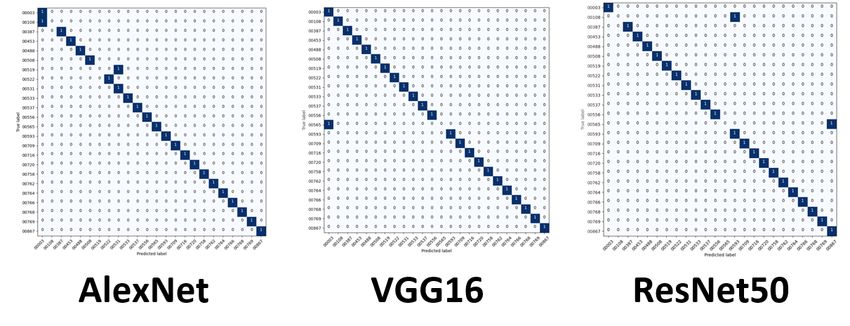
Computers 2021, 10, 113                                                                                           2 of 24

                          be replicated [10]. Further complications include the approach taken because different
                          techniques can yield different results [10]. Some influences that contribute to these problems
                          are the position, illumination, and expression [1–4,8,12,13]. Other influences include
                          pose angles [1,8], camera distance, head size, rotation, angle, and direction [3,5,6]. The
                          introduction of aging, scaling, accessories, occlusion [1,13], and hair [5] makes capturing
                          these varying scales more difficult [14]. Limitations on the image quality such as noise,
                          contrast [15], resolution, compression, and blur [12] also contribute to facial recognition
                          inaccuracies.
                                Although image collection has some varying problems, machine and deep learning are
                          relatively reliable [16] learning algorithms capable of handling large datasets available for
                          research and development [17]. Plenty of facial recognition algorithm variants exist [18,19],
                          and together these algorithms can improve human capabilities in security, medicine, social
                          sciences [17], marketing, and human–machine interface [20]. These algorithms possess
                          the ability to detect faces, sequence, gait, body, and gender determination [19], but still,
                          trained algorithms can produce skewed results [16,17]. These uneven results often lead
                          to a significant drop in performance [16] that can raise concerns about fairness [20]. With
                          the reputation of companies that use facial recognition at stake, many ethical concerns
                          have been raised because of the underrepresentation of other races in existing datasets [16].
                          Inconsistent model accuracy limits the applicability to non-white faces [17], and the dataset
                          contributes to demographic bias [16]. Existing databases and algorithms are insufficient
                          for training due to the low variability in race, ethnicity, and cultures [20]. Most datasets
                          are not labeled for ethnicity [13], and unknown performance [20] and controversial biased
                          models are a result of utilizing these datasets [13].
                                The use of limited models contributes to false matches, low adequacy, fairness, and
                          reliability concerns [20]. Many experiments have observed these results and marked
                          present mostly in faces with a higher melanin presence [16,21]. Convolutional neural
                          networks have improved the capabilities of algorithms [13]. However, there is still much
                          room for group fairness in datasets to mitigate the bias that has existed for decades leading
                          to algorithms suffering from demographical performance bias that provides an imbalance
                          to specific groups of individuals [22]. As racist stereotypes exist, there is a need to avoid
                          mislabeled faces and achieve greater race classification accuracy [23]. Utmost importance
                          should be placed on how human attributes are classified [17] to build inclusive models
                          while considering the need for diversity in datasets [21]. Substantial importance should
                          be emphasized that models need to be diverse due to being trained on large datasets with
                          many variations [13]. The results are algorithms and techniques that mitigate bias [20].
                                The results include an imbalance for some races and demographical bias against
                          specific ethnicities. Considering these inequalities, we investigate and evaluate racial
                          discrimination in facial recognition across the various machine and deep learning models.
                          The findings and results will allow us to discover existing bias with repeatable observations
                          and if any algorithms outperform others while mitigating any bias.
                                Continuing previous research in [23], we continue to measure and evaluate the ob-
                          servable bias resulting from utilizing the five traditional machine learning models and
                          techniques. Replicating the initial approaches and datasets used with conventional algo-
                          rithms, we repeat the previous steps and conduct similar experiments with the three deep
                          learning algorithms. Collecting the results from the deep learning models, we perform
                          identical evaluation and bias measurements. Collecting results for each algorithm used al-
                          lows us to compare performance, accuracy, and bias to evaluate the efficiency of algorithms.
                          We present our findings in hopes of making a meaningful contribution to the decades-old
                          computer vision problem and facial recognition fields. Our collected contributions are:
                          •    Evaluation of racial bias across five machine learning algorithms using racially imbal-
                               anced and balanced datasets.
                          •    Evaluation of racial bias across three deep learning algorithms using racially imbal-
                               anced and balanced datasets.
                          •    Evaluation and comparison of accuracies and miss rates between tested algorithms.
Computers 2021, 10, 113                                                                                            3 of 24

                          •    Report the algorithms that mitigate the bias the most.

                          2. Background
                               As humans, we can quickly identify a face and recognize an individual within a short
                          time. The idea of facial recognition is done daily, and with minimal effort that we may
                          consider this task easy. As time passes, we may see a face that seems familiar, but may
                          not recall the name of the individual even though we recognize them. The introduction of
                          computers to assist with this computer vision problem allows the capabilities to expand
                          to remember substantially more faces. However, once it seemed easy for a human, it is a
                          much more complicated task for a machine. The initial concept of facial recognition was a
                          straightforward task with an obvious solution. The solution involved obtaining an image
                          and precisely identifying or determining if the image matched against a database of stored
                          images. However, four main obstacles present unique problems for facial recognition to
                          be completed successfully. The first problem is the complexity of the task itself, where the
                          next problem is shown in the influences on the images themselves. The final problematic
                          area for facial recognition lies within the algorithms and datasets. Together these problems
                          combined present a unique problem that is observable in technology that is used every day.

                          2.1. Complexity
                               For a human to visually recognize a face, we first must observe a face with our eyes,
                          and this image is introduced to the ocular nerve. The idea is then sent to the brain, where
                          the brain retrieves the name that we associate with that face if it is recallable. Many systems
                          are working in tandem, and we often do not realize the complexity of a task that appears
                          so simple. For a computer to first remember an image, it must convert that image into
                          a data structure to compare against others [24]. In our case, we introduce a traditional
                          photograph that we transform into an array of numbers to represent each image’s pixel.
                          After converting the pictures, they are then stored for comparison against additional photos.
                          Calculating values for each pixel is a complex task that can involve thousands or millions
                          of steps to complete depending on image size and quality, especially if you consider that
                          each pixel comprises values representing the red, green, and blue values within itself.

                          2.2. Influences
                               Influences are one of the most varying items that severely impact facial recognition.
                          The typical three items referenced in the field are pose, illumination, and expression (PIE).
                          Most conventional images are collected by a photographer using a fixed camera with a
                          seated individual in precisely controlled lighting. However, if we suddenly consider any
                          image as usable, then a candidate for recognition may be standing, seated, or involved in an
                          action. The lighting could be too bright or too dark, depending on the location of the image
                          collection. Considering expression is another barrier because viewing traditional images
                          may have a subject smiling. However, your system would still need to recognize your face
                          if you were in a bad mood or had a different expression such as surprise, shock, or pain.
                          Additional items that present problems are aging, angle, scaling, accessories, and occlusion.
                          As we age, our face has subtle changes that make facial recognition more difficult because
                          the look is slightly different. Using a mobile device to collect images can allow individuals
                          to manage their appearance. Still, there is no guarantee that they will hold the camera
                          perfectly level or at an exact distance away from their face. Accessories such as jewelry,
                          glasses, facial hair, hairstyles, and hair color can support the occlusion of a look, making
                          this complex task even more difficult. During our research, the topic of masks as a new
                          item that covers faces and their impact on systems was discussed. During the pandemic a
                          mask was introduced as a new accessory that covers a considerable amount of a face.
Computers 2021, 10, 113                                                                                          4 of 24

                          2.3. Algorithms
                               Once a facial recognition system is in use and the influences and complexity issues
                          have been considered. The next item that impacts the miss rates, hit rates, and the system’s
                          accuracy is the algorithms themselves. Algorithms can contain several factors that may
                          obtain results that are not precise. An algorithm is designed to do what it is programmed
                          to do, and it will consistently execute as it is programmed. However, these algorithms are
                          created by humans, and this underlying problem can surface within the intended results
                          of an algorithm. Psychologists have studied this as something that humans instinctively
                          do from childhood. Where humans interact with what they are familiar with or interact
                          with more frequently. This phenomenon is observable in facial recognition algorithms
                          designed in Eastern and Asian countries when compared against American counterparts.
                          An algorithm designed in an Asian country will have some influence from its Asian
                          designer and their daily interaction with other community members. This bias will likely
                          result in a system that performs better for those types of individuals. Especially measuring
                          results within that community when compared to other nations. Using inferior algorithms
                          leads to skewed results, performance degradation, and applicability limitations. Biased
                          algorithms can produce results that are not meaningful when considering other outside
                          contributions. This bias demonstrates the need for careful thought when designing an
                          algorithm to be inclusive for all intents and purposes.

                          2.4. Datasets
                                If the algorithm has carefully been planned during implementation, it is a particular
                          assumption that it is only as good as the dataset it utilizes. Most datasets do not have
                          labels for races, ethnicity, and demographics. Training of this type of dataset will yield an
                          inaccurate model. This error would also lead to false matches and poor adequacy. Other
                          obstacles in datasets include the fact that a nation may comprise many different races.
                          Combining a similar race as one nationality complicates the accurate estimation of a specific
                          demographic. For example, Malaysia is a multi-racial composition country with many
                          races that all identify as Malaysian. Our dataset included more than 1000 test subjects,
                          but we could only retrieve approximately twenty Black individuals with more than ten
                          available images. There is an obvious imbalance and underrepresentation of specific races,
                          ethnicities and, nationalities while surveying available datasets for research.
                                Many datasets exist and are available for research and development [10]. However,
                          facial recognition requires many images of each subject, creating an immediate complication
                          for this type of research. Our study utilizes the FERET [25,26] dataset, a publicly available
                          dataset with access granted from the National Institute of Standards and Technology
                          (NIST). Our selected dataset contained 1208 subjects. However, when examining the
                          available images, the number of subjects with many images was predominantly White. This
                          imbalance immediately impacted our research methods and processes, and the limitations
                          for other races were noticeable. Only a few datasets contain many images of the same
                          individual, predominantly comprised of celebrities [3]. Although many datasets are
                          available, they lack the appropriate labeling and classifications that algorithms need to
                          train and test against successfully. Properly documenting existing datasets would be a
                          never-ending process, and still, the datasets would be insufficient for certain demographic
                          and racial representations. An image revolution or campaign is needed to gather lots of
                          images so that datasets become more diverse and inclusive with representations of all
                          walks of life. Tuned datasets such as FairFace and DemogPairs successfully mitigated
                          existing racial and demographic bias [3,7].

                          2.5. Machine Learning Algorithms
                               Machine learning algorithms make informed decisions by parsing data and learning
                          from the collected data [27]. Typically, these techniques are used to examine large databases
                          to extract new information as a form of data mining. Many large companies use machine
                          learning to provide an improved user experience in human–computer interaction. These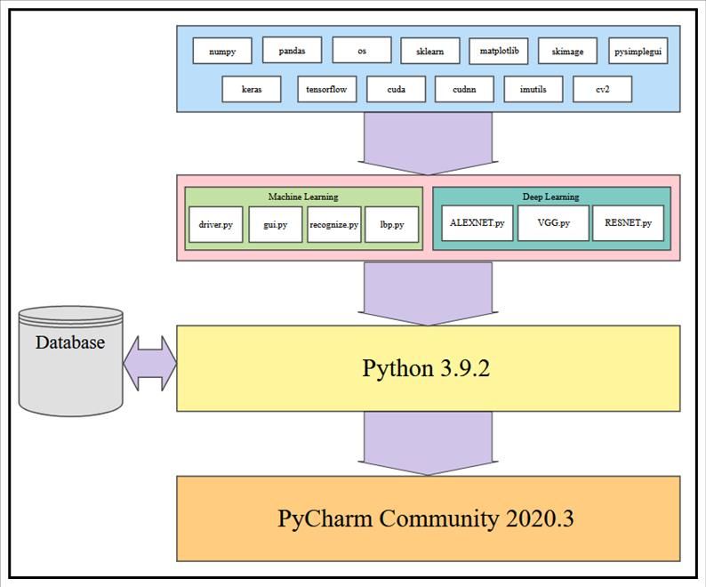
Computers 2021, 10, 113                                                                                          5 of 24

                          improvements may include a recommendation based upon preferences or suggestions
                          based on previous selections [27]. Machine learning algorithms require outside exchange if
                          corrections or adjustments are necessary. A general analogy to envision a machine learning
                          algorithm can be demonstrated by using a flashlight. If we teach the flashlight with a
                          machine learning model, it will understand light and dark. If provided with the word dark,
                          the flashlight will come on. The opposite will occur if the word light is used. However,
                          if presented with a word or phrase it has not learned, such as dim, it will not function
                          and require additional adjustments to accommodate the new expression [27]. Gwyn
                          et al. [23] studied traditional machine learning techniques prompting further research
                          in facial recognition, specifically regarding racial bias. We have chosen Support Vector
                          Classifier (SVC), Linear Discriminant Analysis (LDA), K-Nearest Neighbor (KNN), Decision
                          Trees (DT), and Logistic Regression (LR) algorithms from [23]. These algorithms are used for
                          several applications and the approaches can vary such as regression, clustering, dimension
                          reduction and image classification. For our study, we choose to apply these algorithms
                          using classification methods and do not combine or use them in tandem to produce
                          observable results for each algorithm.
                                Using SVC, image classification for a multi-class approach is achieved by constructing
                          linear decision surfaces using high-dimensional features mapped by non-linear input [23].
                          LDA is used as a classifying approach by using a normally distributed dataset and project-
                          ing the input to maximize the separation of the classes [23]. Classification utilizing KNN is
                          achieved by assigning classes to the output. The designation is concluded by the overall
                          counts of its nearest cohorts, and the class assignment goes to the class with the most
                          common neighbors [23]. The DT approach yields its classifications as a structure and treats
                          each child or leaf as a subset without statistical reasoning [23]. The LR approach reaches
                          the classification by considering the probability that a class exists where the outcome is
                          that a training image and a test image belong to the same class [23].

                          2.6. Deep Learning Algorithms
                                Much like machine learning was a form of data mining, deep learning algorithms are
                          a subset of machine learning that functions similarly, but with differing capabilities [27].
                          If a deep learning algorithm returns an incorrect prediction, the model itself will correct
                          it internally. These algorithms may also use selections and preferences initially, but once
                          deployed, they learn solely on the model and what it was trained on to predict and
                          correct upon [27]. Vehicles that drive automatically or features on them that make lane
                          corrections, braking, and accident avoidance autonomously are some examples of deep
                          learning algorithms in use. We can continue the flashlight analogy to better assist with
                          understanding deep learning algorithms. The light would not need a keyword to associate
                          with action because it would compute from its model and learn to be on or off when
                          required [27]. For our continuing research, we have chosen AlexNet, VGG16, and ResNet50
                          deep learning algorithms.

                          3. System and Experimental Design
                               The similarities in the construction of our machine learning and deep learning algo-
                          rithms, as shown in Figure 1, denotes the similarities between the two. Both algorithms
                          follow a similar route for execution and use inputs to test for successful recognition. Both
                          algorithms store the results of their training for future comparison and testing. Still, the
                          most notable differences are the number of iterations or epochs that deep learning uses to
                          learn and perform better. Machine learning algorithms take input and apply the settings
                          and execute a mathematically complex algorithm once.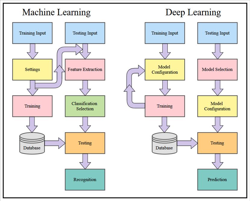
Computers 2021, 10, x FOR PEER REVIEW 6 of 24
Computers 2021, 10, 113 6 of 24
learning uses to learn and perform better. Machine learning algorithms take input and
apply the settings and execute a mathematically complex algorithm once.
Figure 1. Overview of learning algorithms.
Figure 1. Overview of learning algorithms.
3.1. System Design and Architecture
3.1. System
OurDesign
machine and learning
Architecturealgorithms take images and use them as input to train the
system, as shownlearning
Our machine in Figurealgorithms
1. After initialization,
take imagesthe andgraphical
use themuserasinterface
input to(GUI)traincollects
the
testing variables, so identical approaches are used. The following
system, as shown in Figure 1. After initialization, the graphical user interface (GUI) steps are for the system
to train
collects on inputs
testing of balanced
variables, or imbalanced
so identical approaches datasets
are used. andThe
savefollowing
them to astepsdatastore.
are forDuring
the
the testing portion, the system takes the images as input and applies
system to train on inputs of balanced or imbalanced datasets and save them to a datastore. the same setting used
for training.
During the testingThe portion,
system extracts the features
the system takes the and bringsas
images theinput
classification
and applies selection
the samefor the
desired algorithms. The testing phase compares the calculated image
setting used for training. The system extracts the features and brings the classification to the saved training
imagesfor
selection to the
recognize.
desired algorithms. The testing phase compares the calculated image to
the saved trainingapproach
A similar images toisrecognize.
used for the deep learning algorithms where input is used for
training. The model
A similar approach is usedof the algorithm
for the deepto be used isalgorithms
learning constructed. The input
where training iterates
is used for or
cycles for a selected number of epochs. During the revolutions of
training. The model of the algorithm to be used is constructed. The training iterates or each period, the system
can for
cycles validate the training
a selected numberfor of accuracy and improve
epochs. During predictions
the revolutions of on each
each iteration.
period, Once the
the system
training is completed, the datastore is used to save the trained model, as shown in Figure 1.
can validate the training for accuracy and improve predictions on each iteration. Once the
training is completed,
3.2. System Software the datastore is used to save the trained model, as shown in Figure
1.
Continuing prior research [23], Python® was the language used, which was a require-
ment for our continuing research and experimentation. Python is a powerful programming
3.2. System Software
tool that granted us access to many libraries that assisted with implementing this project.
Continuing
Those imported prior research
libraries [23],Pandas,
include PythonNumPy,
® was the language used, which was a
OS, Scikit-Learn, Matplotlib, Keras,
requirement
TensorFlow, forCUDA,
our continuing
and cuDNN, research
as shown andinexperimentation.
Figure 2. Python is a powerful
programming
Pandas tool that granted
is a powerful utilityusto access to many libraries
collect DataFrame that and
information, assisted
NumPy withwas
implementing this project. Those imported libraries include Pandas, NumPy,
successful in data structure manipulation. Tools included by importing Scikit-Learn include OS, Scikit-
Learn, Matplotlib,
confusion Keras,
matrices andTensorFlow, CUDA,
built-in metrics and cuDNN,
reporting. as shown
Matplotlib wasin Figurefor
utilized 2. feedback
and graphing during code execution. The subsequent imports were the game changers
for this project. The Keras neural network library has an extensive catalog of tools built
on the open-source library of TensorFlow. These high-level Application Programming
Interfaces (APIs) assisted in layering, pooling, metric reporting, model construction, and
optimization. The addition of the CUDA and cuDNN imports is where the significant drop
in runtime occurred. After configuring them properly, they allow the GPU to be utilizedComputers 2021, 10, 113 7 of 24
in tandem with the CPU. Overall runtimes significantly drop by more than 75%. Each of
Computers 2021, 10, x FOR PEER REVIEW 7 of 24
our model interpretations is paired with some of these imports and our FERET dataset
compilation. The existing code implementations for our experimentation are conducted in
Python 3.9.2 using PyCharm Community Edition 2020.3.
Figure 2. Software architecture.
Figure 2. Software architecture.
3.3. Evaluation Plan
Pandas
Exploringis this
a powerful utilitythree
topic requires to collect
generated DataFrame information,
datasets and and NumPy
machine learning was
algorithms
successful in data structure manipulation. Tools included by importing
to compare performance and results against each. We conducted a plethora of research to Scikit-Learn
include confusion
collect images and matrices
place them andintobuilt-in
groupsmetrics
that willreporting. Matplotlib
yield observable wasthat
results utilized for
hopefully
feedback and graphing during code execution. The subsequent imports
will have a meaningful contribution to the facial recognition field. Sampling is sourced were the game
changers for thisdataset
from the FERET project. The Keras diverse,
emphasizing neural network
inclusivelibrary
imageshaswithanracial
extensive catalog
variations. Threeof
tools built
datasets areon the open-source
distributed to yield alibrary
balanceofofTensorFlow.
equal amounts These high-level
of image Application
representations for
Programming
each race. The Interfaces
other two sets(APIs)
are assisted in to
distributed layering, pooling,
weigh heavier metric areporting,
towards particular model
race or
construction,
ethnicity. Theand optimization.
datasets The addition
are then analyzed withof the CUDAand
algorithms, andperformance
cuDNN imports is where
is rated on the
the significant drop in runtime occurred. After configuring them properly,
accuracy of prediction modeling. Additional metric measurements include precision, recall, they allow the
GPU to be utilized in tandem with the CPU. Overall runtimes significantly
and F1 scoring. Algorithms and models utilized are Support Vector Classifier (SVC), Linear drop by more
than 75%. EachAnalysis
Discriminant of our model
(LDA), interpretations is paired(KNN),
K-Nearest Neighbors with some of these
Decision imports
Trees (DT), and our
Logistic
FERET dataset
Regression (LR),compilation. The existing
AlexNet, VGG16, code implementations
and ResNet50. In the initial for our on
testing experimentation
the sample of
are conducted
24 subjects, weinthen
Python
alter3.9.2 using PyCharm
the dataset to be biased Community
towards aEdition 2020.3.
particular race. For dominant
set 1, we choose 16 topics to represent the Black classification and 8 subjects to describe
3.3.
the Evaluation Plan We make a similar comparison for the next phase in experimentation,
White variety.
but this time wethis
Exploring complement experiment
topic requires three2.generated
For dominant set 2, we
datasets andchoose 16 subjects
machine learning to
represent the
algorithms White and
to compare 8 subjects toand
performance define the against
results Black classification.
each. We conducted a plethora of
Theto
research weighting for each
collect images andscenario is as follows:
place them into groups that will yield observable results
• hopefully
that Balanced—12 willBlack
havesubjects vs. 12 White
a meaningful subjects; to the facial recognition field.
contribution
• Dominant
Sampling Set 1—16
is sourced fromBlack subjects
the FERET vs. 8 emphasizing
dataset White subjects; diverse, inclusive images with
•
racialDominant
variations.Set 2—8 datasets
Three Black subjects vs. 16 White
are distributed subjects.
to yield a balance of equal amounts of
imageEveryone
representations for each 12
has an available race. The other
images because twoof sets are distributed
the limitations of ourtodataset.
weigh heavier
Initially,
towards
we selecta11
particular
ideas for race
thoseoravailable
ethnicity. The datasets
algorithms areon
to train then
andanalyzed with algorithms,
set the remaining image as
and performance
the image is rated
to test against foron the accuracy
accuracy. We then of remove
prediction modeling.
3 photos Additional
to eliminate metric
influences of
measurements include precision, recall, and F1 scoring. Algorithms and models utilized
are Support Vector Classifier (SVC), Linear Discriminant Analysis (LDA), K-Nearest
Neighbors (KNN), Decision Trees (DT), Logistic Regression (LR), AlexNet, VGG16, and
ResNet50. In the initial testing on the sample of 24 subjects, we then alter the dataset to beComputers 2021, 10, 113 8 of 24
position, illumination, expression, or occlusion to explore accuracy. This setup allows us to
test on the original image, but train on only 8 images. To mitigate the limitations of our
dataset, we then revisited our initial training set that contained 11 images and augmented
them. This method allows us to create additional pictures by inverting the original copies
and giving us 22 photos to train.
The dataset configurations for each experimental scenario are:
• Eight images for training and 1 image for testing per subject;
• Eleven images for training and 1 image for testing per subject;
• Twenty-two Images for training and 1 image for testing per subject.
3.4. Evaluation Procedure
The evaluation involves careful consideration to continue previous research conducted
in [23]. Initial research performed was explicitly applied to the field of facial recognition
in general. Moving forward, we aim to use that research to observe existing bias and
identify approaches to mitigate these inaccuracies. Metrics involved in these evaluations
will include accuracy, precision, recall, F1 score, hit rates, and miss rates.
Our experimentation involves very precise steps that must be repeated, so the col-
lected results are free from uncontrolled changes. The steps we have followed for each
algorithm are:
1. Select the algorithm;
2. Select the dataset;
3. Measure the metrics;
4. Repeat steps 2 and 3 for each dataset with selected algorithm;
5. Repeat entire process for each algorithm.
3.5. Experimental Design
Details regarding machine specifics and methodologies are provided in this section
to give an insight into the technology used. These details will serve as a gauge for others
to compare to when considering turn-around and runtimes. Our experimentation was
performed on a Dell® Alienware® Aurora® Ryzen® machine running a Windows 10® oper-
ating system. The Central Processing Unit (CPU) is an AMD® Ryzen® 9 3900XT 12-Core
Processor 3.79 GHz. The available memory includes a 512 Gigabytes (GB) Solid State
Drive (SSD) and 32 Gigabytes Random Access Memory (RAM). It consists of an NVIDIA®
GeForce® RTX 2070 8GB GD DR6 for graphics that significantly contributed to expediting
experimentation after installing the required libraries. The Integrated Development Envi-
ronment (IDE) used was PyCharm Community Edition 2020.3® , a product of JetBrains® .
Code implementation for our project was designed using Python 3.9.2 using our IDE.
Importing TensorFlow, CUDA and cuDNN allows the machine to use the stream executor
to create dynamic libraries that utilize the graphics card for CPU support. The addition
of these dynamic libraries significantly reduced the overall runtimes of all algorithms.
Before optimizing the configurations, runtimes for the machine learning algorithms took
approximately 180 s to complete depending on the number of images utilized. With the
optimization configuration, the runtimes are reduced to about 32 s for each selected model.
The deep learning algorithms use a sizeable learning epoch, so overall runtimes depend
on that setting. Our generalized settings of 50 periods yield runtimes of approximately
18 min, where our optimized settings reduce that time to around 4 min. Taking averages of
our three deep learning algorithms produces an average of 7 s per epoch.
4. Experimental Results
The collected results yield a comprehensive overview to visualize performance across
the racially imbalanced datasets, much like a sliding scale. Collectively, we document the
results for each algorithm in its category and then compare their results between the two
types of algorithms.4. Experimental Results
The collected results yield a comprehensive overview to visualize performance
across the racially imbalanced datasets, much like a sliding scale. Collectively, we
Computers 2021, 10, 113 9 of 24
document the results for each algorithm in its category and then compare their results
between the two types of algorithms.
4.1. Racial Bias across ML Algorithms
4.1. Racial Bias across ML Algorithms
Our results began with the execution of our algorithms using the first dataset with
Our results began with the execution of our algorithms using the first dataset with
eight training images. This approach gives us eight ideas to train on and one image to test
eight training images. This approach gives us eight ideas to train on and one image to test
for accuracy. We performed the experiments as directed on our balanced dataset to serve
for accuracy. We performed the experiments as directed on our balanced dataset to serve
as a baseline for comparison. Support Vector Classifier was the superior algorithm of the
as a baseline for comparison. Support Vector Classifier was the superior algorithm of the
fivemachine
five machinelearning
learningchoices.
choices. However,
However,the
theaccuracy
accuracybarely
barelysurpassed
surpassedthe
the80%
80%mark,
mark,as
as
shown in Figure 3, which is well below the industry standard and user expectations.
shown in Figure 3, which is well below the industry standard and user expectations.
Figure 3. ML accuracies with balanced dataset and 8 training images.
Figure 3. ML accuracies with balanced dataset and 8 training images.
Another notable result is the low level of performance for the other algorithms, espe-
ciallyAnother notable
the K-Nearest result is algorithm
Neighbors the low level
barely ofsurpassed
performance for the
the 50th other algorithms,
percentile. Applying
especially the K-Nearest Neighbors algorithm barely surpassed
this experiment to the different datasets demonstrates the importance of the the 50thdataset.
percentile.
We
Applying
Computers 2021, 10, x FOR PEER REVIEW
repeat this experiment
the steps to the
for each dataset todifferent
measure datasets demonstrates
the differences the importance
while exhibiting 10ofof the
bias towards 24
adataset.
specificWe repeat
race. Thesethetypes
stepsoffor each dataset
experiments to measure
differ slightly the
fromdifferences
our baselinewhile exhibiting
results. You
biassee
can towards a specific
that the dominant race. Thesetowards
dataset types of Blacks
experiments differ slightly
has declining fromfor
accuracies ourDecision
baseline
results.
Trees and
compared Youto can
thesee
Logistic that the
White dominant
Regression.
dataset The dataset
two
yielding towards
datasets
slightly in Blacks
Figure
better 4has declining
yield
results similar
when accuracies
results
applied to com-
ourfor
Decision
pared to Trees
the and
White Logistic
dataset
machine learning algorithms. Regression.
yielding The
slightly two
better datasets
results in Figure
when 4
appliedyield
tosimilar
our results
machine
learning algorithms.
Figure 4. ML accuracies with imbalanced datasets and 8 training images.
Figure 4. ML accuracies with imbalanced datasets and 8 training images.
The results for this first experiment are not very different, but considering the results
already demonstrates a potential problem. We compile the accuracies for each algorithm,
and the results show that deviating from a fair and balanced approach can yield unwantedComputers 2021, 10, 113 10 of 24
The results for this first experiment are not very different, but considering the results
already demonstrates a potential problem. We compile the accuracies for each algorithm,
and the results show that deviating from a fair and balanced approach can yield unwanted
side-effects, as shown in Table 1. The results show that using a dataset that is dominant
towards Blacks underperforms compared to its cohort. Specific algorithms perform better
than others, but averages demonstrate an unbiased insight that a problem exists.
Table 1. Accuracies of machine learning algorithms using 8 training images.
Accuracy Table Datasets
ML Algorithm WD RBAL BD
SVC 83% 83% 83%
LDA 67% 58% 63%
KNN 71% 54% 54%
DT 63% 67% 63%
LR 63% 63% 63%
AVERAGES 69% 65% 65%
Considering the number of miss rates for each race while simultaneously monitoring
the dataset type provides a different metric that reinforces the notion that bias in a dataset
contributes to uneven results, as shown in Table 2.
Table 2. Average ML miss rates for datasets using 8 training images.
ML Algorithms Miss Rates for Datasets WD RBAL BD
Average Black Miss Rate 32.50% 38.33% 32.50%
Average White Miss Rate 30.00% 31.67% 40.00%
The Difference of Average Miss Rates 2.50% 6.66% 7.50%
Finally, we evaluate the other available metrics of precision, recall, and F1 scoring.
A complete scoring metrics table is in [28], and for analysis purposes, we provide the
averages in Table 3.
Table 3. Additional ML metrics precision, recall and F1.
ML Metrics
WD RBAL BD
Averages
Precision 69% 66% 65%
Recall 100% 100% 100%
F1 82% 79% 78%
Across the datasets, average metrics increase and decrease when changing from our
balanced baseline dataset. When deviating towards a dataset that is White dominant (WD),
the metric averages increase for precision and F1 scores, and the opposite occurs when a
Black prevailing dataset is used. The collected results from the experimentation using the
first dataset are compiled for further analysis and comparison.
The next portion of our experiments will repeat the steps previously completed for
the eight training images. Still, instead, this time, we replace the eight training images with
our dataset with 11 pictures to train. The thought for this approach was that the addition
of more training images would allow the algorithms to perform better and achieve higher
accuracies and performance metrics. We first establish our baseline by using the dataset
that has one representation for each racial profile. We utilize the same five machine learning
algorithms, and the results are shown in Figure 5.The next portion of our experiments will repeat the steps previously completed for
the eight training images. Still, instead, this time, we replace the eight training images
with our dataset with 11 pictures to train. The thought for this approach was that the
addition of more training images would allow the algorithms to perform better and
Computers 2021, 10, 113
achieve higher accuracies and performance metrics. We first establish our baseline11 of 24
by
using the dataset that has one representation for each racial profile. We utilize the same
five machine learning algorithms, and the results are shown in Figure 5.
Figure5.5.ML
Figure MLaccuracies
accuracieswith
withbalanced
balanceddataset
datasetand 11 11
and training images.
training images.
When
Whencomparing
comparingthe results
the to our
results previous
to our experiments,
previous the accuracies
experiments, have im-
the accuracies have
proved for all algorithms. Support Vector Classifier is still the top achiever with 92%
improved for all algorithms. Support Vector Classifier is still the top achiever with 92%
accuracy, and K-Nearest Neighbors is still the lowest performer at almost 70%. With our
accuracy, and K-Nearest Neighbors is still the lowest performer at almost 70%. With our
baseline established, we can compare the results of each imbalanced dataset and see im-
baseline established, we can compare the results of each imbalanced dataset and see
mediate changes, as shown in Figure 6. The most significant difference shown here 12
Computers 2021, 10, x FOR PEER REVIEW is of
that
24
immediate
SVC changes,
performs as shown
at 96% when in with
paired Figure
the6.White
The most significant
dataset. difference
All the other shown
algorithms here is
barely
that SVC
achieve performs at 60%
approximately 96% when
whenusing
paired thewith thedataset.
Black White dataset. All the other algorithms
barely achieve approximately 60% when using the Black dataset.
Figure 6. ML accuracies with imbalanced datasets and 11 training images.
Figure 6. ML accuracies with imbalanced datasets and 11 training images.
In this round of experimentation, we find that the averages for each dataset have
In this round of experimentation, we find that the averages for each dataset have
increased. However, when using the Black dataset, the standards remain in the 60-percentile
increased. However, when using the Black dataset, the standards remain in the 60-
range. The balanced dataset and White dominant (WD) dataset improved accuracies to
percentile
exceed the range. The balanced
mid-70-percentile, datasetinand
as shown White
Table 4. dominant (WD) dataset improved
accuracies to exceed the mid-70-percentile, as shown in Table 4.
Table 4. Accuracies of machine learning algorithms using 11 training images.
Accuracy Table Datasets
ML Algorithm WD RBAL BD
SVC 96% 92% 88%
LDA 71% 71% 63%Computers 2021, 10, 113 12 of 24
Table 4. Accuracies of machine learning algorithms using 11 training images.
Accuracy Table Datasets
ML Algorithm WD RBAL BD
SVC 96% 92% 88%
LDA 71% 71% 63%
KNN 83% 67% 67%
DT 71% 79% 54%
LR 71% 71% 63%
AVERAGES 78% 76% 67%
Our miss rate findings indicate an overall decline and are likely due to better training
because of additional training images. The miss rate percentages are still well beyond what
a user may expect or desire. The gap between them statistically shows bias towards the
White dataset, as shown in Table 5.
Table 5. Average ML miss rates for datasets using 11 training images.
ML Algorithms Miss Rates for Datasets WD RBAL BD
Average Black Miss Rate 25.00% 25.00% 33.75%
Average White Miss Rate 20.00% 23.33% 32.50%
The Difference of Average Miss Rates 5.00% 1.67% −1.25%
Again, we consider additional metrics to gain an insight that can support our ini-
tial findings, and again we see that using the averages in Table 6. Using a weighted
dataset towards Blacks yields lower performance metrics for accuracy, precision, and F1
scores. Ref. [28] includes the complete scoring metrics table since we use the averages for
generalized analysis.
Table 6. Additional ML metrics precision, recall and F1.
ML Metrics
WD RBAL BD
Averages
Precision 78% 76% 67%
Recall 100% 100% 100%
F1 87% 86% 79%
We attempted to circumvent the limitations presented to us regarding our dataset
for our next round of experimentation. We took the initial 11 images for training and
augmented them to give us 22 representations to train the algorithms with more images.
In this instance, we used the inverse representation of each available image and created
a new dataset for training. Again, the expectation is that more training images will yield
better performance and lower miss rates. We use the same approach and initially use
the balanced dataset to establish a baseline for comparison purposes. We now see that a
balanced dataset has achieved 96% accuracy for this iteration, as shown in Figure 7. These
baseline results show improvement, but are still lacking accuracies that should be expected
in facial recognition.new dataset for training. Again, the expectation is that more training images will yield
better performance and lower miss rates. We use the same approach and initially use the
balanced dataset to establish a baseline for comparison purposes. We now see that a
balanced dataset has achieved 96% accuracy for this iteration, as shown in Figure 7. These
Computers 2021, 10, 113 baseline results show improvement, but are still lacking accuracies that should 13 of 24 be
expected in facial recognition.
Figure 7.
Figure ML accuracies
7. ML accuracies with
withaabalanced
balanceddataset
datasetand
and2222
training images.
training images.
With our baseline results established, we then move on to compare the results of each
With our baseline results established, we then move on to compare the results of each
imbalanced dataset. Each dataset used was weighted to favor Blacks or Whites, and the
imbalanced dataset. Each dataset used was weighted to favor Blacks or Whites, and the
expectations are that more training images would yield higher accuracy. This time, we see
expectations
that using theare that dominant
White more training
(WD)images
datasetwould
yieldsyield higher
better accuracy.
accuracies whenThis time, we
compared to see
that using the White dominant (WD) dataset yields better accuracies when compared
the previous experiments. Still, we also note that the Black counterpart has some declines to
Computers 2021, 10, x FOR PEER REVIEW 14 of 24
the previous experiments. Still, we also note that the Black counterpart has some
in performance, as shown in Figure 8. Although the graphs appear similar, the y-axis for declines
in
theperformance,
White portionashas
shown
a maxinvalue
Figureof 8. Although
100, where thethe graphs
max valueappear
for the similar, the y-axis
Black graph is 90. for
the White portion has a max value of 100, where the max value for the Black graph is 90.
Figure8.8.ML
Figure MLaccuracies
accuracieswith
withimbalanced
imbalanceddatasets
datasetsand
and 22
22 training
training images.
images.
We
Weinvestigate
investigatethethe
averages of all
averages of the
all algorithms whilewhile
the algorithms considering race, and
considering race,a notice-
and a
able performance
noticeable gap is shown
performance in Tablein7.Table 7.
gap is shown
This difference is between the Black dominant (BD) dataset and the others, with the
other
Tabletwo outperforming
7. Accuracies by 10%.
of machine Observations
learning for this
algorithms using round of
22 training experimentation include
images.
the accuracy improvements for each dataset, but a worsening divide in performance. This
Accuracy Table Datasets
problem is dually observable in the miss rate calculations. Overall, our miss rates have
declined, but the margin has increased when considering theRBAL
ML Algorithm WD differences, as shownBDin Table 8.
SVC 96% 96% 92%
LDA 71% 71% 63%
KNN 83% 71% 63%
DT 75% 79% 67%
LR 71% 79% 58%Computers 2021, 10, 113 14 of 24
Table 7. Accuracies of machine learning algorithms using 22 training images.
Accuracy Table Datasets
ML Algorithm WD RBAL BD
SVC 96% 96% 92%
LDA 71% 71% 63%
KNN 83% 71% 63%
DT 75% 79% 67%
LR 71% 79% 58%
AVERAGES 79% 79% 69%
Table 8. Average ML miss rates for datasets using 22 training images.
ML Algorithms Miss Rates for Datasets WD RBAL BD
Average Black Miss Rate 17.50% 20.00% 28.75%
Average White Miss Rate 22.50% 21.67% 37.50%
The Difference of Average Miss Rates −5.00% 1.67% 8.75%
The same conclusion can be made when considering the additional metrics. The
introduction of other images has allowed the performances to improve, but comparing the
versions, shows an existing difference based on racial weighting in the datasets. Table
Computers 2021, 10, x FOR PEER REVIEW 15 of 249
provides the averages for the metrics, and complete findings and scoring metrics are in [28].
Table 9. Additional ML metrics precision, recall and F1.
Table 9. Additional ML metrics precision, recall and F1.
ML Metrics
ML Metrics Averages WD
Averages WD RBAL RBAL BD
BD
Precision 79% 79% 69%
Precision 79% 79% 69%
Recall 100% 100% 100%
Recall 100% 100% 100%
F1 88% 88% 81%
F1 88% 88% 81%
4.2. Racial Bias across DL Algorithms
4.2. We
Racial Biascareful
were across DL Algorithms
to use the exact dataset representations and configurations for the
We were careful
experimentation to use
for deep the exact
learning dataset representations
algorithms. and configurations
Our initial testing followed the for the
same
experimentation for deep learning algorithms. Our initial testing followed
approaches and methods, and we first applied the AlexNet deep learning algorithm using the same
approaches
the and methods,
eight training and we first
images datasets. applied provides
Matplotlib the AlexNet deep learning
an insight into thealgorithm
model
using the eight training images datasets. Matplotlib provides an insight
performance for each epoch to visually represent the accuracy and loss of the model. into the model
For
performance for each epoch to visually represent the accuracy and loss of the
these tests, we have also utilized the included confusion matrix support for prediction and model. For
these tests,
accuracy we have also
visualization. utilized
During ourthe included
training, lossconfusion matrix
and accuracy support
metrics arefor prediction
gathered to
and accuracy visualization. During our training, loss and accuracy
generate a visual representation for each epoch, as shown in Figure 9. metrics are gathered to
generate a visual representation for each epoch, as shown in Figure 9.
Figure 9. Validation and loss graph examples.
Figure 9. Validation and loss graph examples.
Ideally, the graphs should show decreasing loss and increasing accuracy for each
cycle. These graphs are general reference material and have minimal differences if the
algorithm performs as desired, and input is applied appropriately, but quickly indicatesComputers 2021, 10, 113 15 of 24
Figure 9. Validation and loss graph examples.
Ideally,
Ideally, the
the graphs
graphs should
should showshow decreasing
decreasing loss
loss and
and increasing
increasing accuracy
accuracy for for each
each
cycle.
cycle. These graphs are general reference material and have minimal differences if
These graphs are general reference material and have minimal differences if the
the
algorithm
algorithm performs
performs asas desired,
desired, andand input
input isis applied
applied appropriately,
appropriately, but
but quickly
quickly indicates
indicates
when
when aa problem
problem arises.
arises. The
The complete
complete accuracy
accuracy andand loss
loss graphs
graphs can
can be
be found
found inin [28].
[28].
The
The confusion matrix is formatted along the y-axis to include the labels that arethat
confusion matrix is formatted along the y-axis to include the labels knownare
known to beThe
to be true. true. The is
x-axis x-axis is formatted
formatted with tagswiththat
tagsrepresent
that represent the prediction
the prediction of the of the
given
given test image based on the training. Ideally, the projections create a diagonal
test image based on the training. Ideally, the projections create a diagonal formation if all formation
ifpredictions
all predictions are accurate.
are accurate. A deviation
A deviation fromdiagonal
from this this diagonal formation
formation indicates
indicates a miss.a Using
miss.
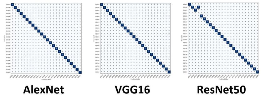
Using our balanced training dataset with eight available images, we generate
our balanced training dataset with eight available images, we generate the results and the results
and immediately
immediately see VGG16
see that that VGG16 onlyone
only has hasmiss,
one miss,
and the and the others
others have
have two two misses,
misses, as shown as
shown
in Figurein Figure
10. The10. The complete
complete confusionconfusion
matrices matrices are in [28].
are in [28].
Computers 2021, 10, x FOR PEER REVIEW 16 of 24
Figure 10. DL confusion matrices using balanced datasets and 8 training images.
Figure DL confusion
10. results
The matrices using
are excellent balanced
if you datasets
recall and 8 training
the previous images.
percentages recorded for
traditional machine learning approaches and models. These balanced matrices serve as
The results
our baseline, andare excellentmatrices
imbalance if you recall the previous
produced similarpercentages
results for recorded for traditional
each model. However,
machine
the learningtakeaway
most notable approaches
fromand models.
these resultsThese balanced matrices
is consistency. One modelservemay
as our baseline,
outperform
and imbalance matrices produced similar results for each model. However, the most
the other, but the models themselves are more consistent across the datasets, as shown in
notable takeaway from these results is consistency. One model may outperform the other,
Figure 11. It appears these types of algorithms do not display a bias for a particular
but the models themselves are more consistent across the datasets, as shown in Figure 11.
dataset.
It appears these types of algorithms do not display a bias for a particular dataset.
Figure 11. DL accuracies on all datasets using 8 training images.
Figure 11. DL accuracies on all datasets using 8 training images.
These consistent results are also observable in the overall averages of the deep learn-
These consistent
ing algorithms. VGG16 results are also observable
did outperform AlexNet andin the overall by
ResNet50 averages
4%, butofthethe deep
general
learning algorithms. VGG16 did outperform AlexNet and
standards between the datasets are equal, as shown in Table 10. ResNet50 by 4%, but the general
standards between
Measuring thethe datasets
miss are equal,
rates does show as shown in
a sizeable Table 10.statistically, but with such
difference
high accuracies, this difference can be misleading. Table 11 shows that it should be
Table 10. Accuracies
expected of deep
that missing morelearning
of thealgorithms usingbecause
race is biased 8 training images.
there are more opportunities to
miss that race.
Accuracy Table Datasets
DL Algorithm WD RBAL BD
AlexNet 92% 92% 92%
VGG16 96% 96% 96%
Resnet50 92% 92% 92%
AVERAGES 93% 93% 93%Computers 2021, 10, 113 16 of 24
Table 10. Accuracies of deep learning algorithms using 8 training images.
Accuracy Table Datasets
DL Algorithm WD RBAL BD
AlexNet 92% 92% 92%
VGG16 96% 96% 96%
Resnet50 92% 92% 92%
AVERAGES 93% 93% 93%
Table 11. Average DL miss rates for datasets using 8 training images.
DL Algorithms Miss Rates for Datasets WD RBAL BD
Average Black Miss Rate 8.33% 5.56% 4.17%
Average White Miss Rate 6.25% 8.33% 12.50%
The Difference of Average Miss Rates 2.08% 2.78% 8.33%
We continue our observations of the eight-training image experiment with the deep
learning algorithms by measuring the additional metrics. Keras allows us to measure
Computers 2021, 10, x FOR PEER REVIEW
many metrics with many variations such as weighted, micro, and macro. To keep 17 ofour
24
comparisons in similar fashions, we will quote the averages using the micro scores because
they are comparable to the machine learning results. Ref. [28] includes the complete
additional
we scoring
look at the metrics.
averages Although
in Table 12, thesome metrics
results are better like
are consistent, thanthe
thepreviously
others, if we look at
reported
the averages
accuracies. in Table 12, the results are consistent, like the previously reported accuracies.
Table 12. Additional DL metrics precision, recall and F1 using 8 training images.
Table 12. Additional DL metrics precision, recall and F1 using 8 training images.
DL Metrics AveragesAverages WD
DL Metrics WD RBAL RBAL BDBD
PrecisionPrecision 97% 97% 97% 97% 97%
97%
Recall Recall 93% 93% 93% 93% 93%
93%
F1 F1 95% 95% 95% 95% 95%
95%
As
Aswewecontinue
continuethe thesame
samemethods,
methods,wewefollowed
followedour ourmachine
machinelearning
learningapproaches,
approaches,
and
and we repeat the previous steps using 11 images for training. This round
we repeat the previous steps using 11 images for training. This round ofof training
training
produced
produced similar loss and accuracy graphs like the first experiment, and the complete
similar loss and accuracy graphs like the first experiment, and the complete
selection
selectionof
ofcharts
chartsisisin
in[28].
[28].When
Wheninvestigating
investigatingaccuracy,
accuracy,we wefirst
firstcompare
compare the
thegenerated
generated
confusion matrices, in Figure 12, for our balanced datasets with 11 training
confusion matrices, in Figure 12, for our balanced datasets with 11 training images. images.
Figure12.
Figure DLconfusion
12.DL confusionmatrices
matricesusing
usingbalanced
balanceddatasets
datasetsand
and11
11training
trainingimages.
images.
The matrices represent our baseline results, and the other matrices are similar, which
The matrices represent our baseline results, and the other matrices are similar, which
indicates minimal differences. The complete library of confusion matrices is in [28]. When
indicates minimal differences. The complete library of confusion matrices is in [28]. When
experimenting with the imbalanced datasets. We find again that the results are consistent,
as shown in Figure 13.You can also read